Unified snr analysis of medical imaging systems

Abstract

The ideal observer signal to noise ratio (snr) has been derived from statistical decision theory for all of the major medical imaging modalities. This snr provides an absolute scale for image system performance assessment and leads to instrumentation design goals and constraints for imaging system optimisation since no observer can surpass the performance of the ideal observer. The dependence of detectable detail size on exposure or imaging time follows immediately from the analysis. A framework emerges for comparing data acquisition techniques, e.g. reconstruction from projections versus Fourier methods in nmr imaging, and time of flight positron emission tomography (tofpet) versus conventional pet. The approach of studying the ideal observer is motivated by measurements on human observers which show that they can come close to the performance of the idea) observer, except when the image noise has negative correlations—as in images reconstructed from projections—where they suffer a small but significant penalty.

1. Introduction

In the past decade the problem of assessing the performance of medical imaging systems has moved from phenomenology towards unification into a mature theoretical and experimental science. The key to this progress has been the recognition that imaging is basically a two-stage process: (i) a data detection or recording stage; and (ii) a processing and display stage. The data detection stage can be quantified exactly from objective measurements on the imaging system and the application of analytical methods from signal detection theory. The display stage is quantified in terms of the task-dependent performance of real observers viewing images with well defined signal parameters and noise characteristics.

Simplification as well as rigour have been brought to this analysis through the introduction of two constructs regarding optimal observation of an image. The first of these is the heuristic concept of the almost ideal or quasi-ideal observer and the second is the rigorous concept of the ideal observer of detected image information; these observers differ in their ability to take into account correctly the image noise correlations. Human observer performance with displayed images is most easily interpreted in terms of the concept of the quasi-ideal observer. The performance of image detection system hardware is assessed directly using the concept of the ideal observer. Since image assessment is always task dependent, a performance task must be specified for either observer.

Our approach requires only a few fundamentals of signal detection theory and the classical imaging measurements, namely the macro or grey scale transfer characteristic, the micro or detail transfer characteristics and the system noise power spectrum at the operating level of interest. From these we derive the task-dependent ideal observer signal to noise ratio (snr_i). Since no observer can surpass the performance of the ideal observer, this leads to design goals and basic constraints for the engineering of imaging systems. We shall present applications of the approach to all of the major medical imaging modalities.

Finally, we shall discuss some results of studies on real observers (human observers). The real observer's performance can be assessed on the same scale used to assess the ideal observer's performance. A comparison of the two then demonstrates just how much real observer performance can be improved. We shall see that real observer performance can come very close to ideal observer performance except in the cases of unprocessed (e.g. unwindowed) low contrast images and of images obtained through projection reconstruction methods, where there is a small but significant penalty. Equivalently, given sufficient image contrast the real observer performance approaches that of the heuristic quasi-ideal observer.

2. The quasi–ideal observer and the ideal observer

We will begin with a heuristic treatment of a quasi- or almost ideal observer and then introduce the rigorous form for the optimal or truly ideal observer. The quasi-ideal observer is a sub-optimal observer who assumes that the image noise is white, i.e. uncorrelated; he is not able to incorporate information on the noise correlations into his decision strategy but is otherwise ideal. The ideal observer, on the other hand, is able to use all of the information in the noisy image sample, including that in the noise correlations. When the noise is in fact white or uncorrelated the quasi-ideal observer is also ideal.

It is well known that image assessment is task dependent, so it is necessary to specify a task for the observer. We begin with the imaging task that is the simplest to analyse, namely that of detecting a specified low contrast signal (lesion) at a specified position in a noisy image. We will consider the ‘yes/no’ experiment in which the observer must decide whether the signal is present or only the noise background is present.

There are three strategies for performing this detection task that can be shown to be equivalent and to be optimal for white noise (Cook and Bernfeld 1967, Whalen 1971).

1. Use the data to calculate the likelihood ratio; this is the same as the a posteriori odds for the alternatives ‘signal plus noise’ or ‘noise alone’ when their a priori probabilities are equal (see Appendix 1 for an example); then, answer ‘yes’ or ‘no’ according to whether the odds exceed a threshold criterion level.

2. Cross correlate the area to be tested for the presence of the lesion with weights—a mask or template—proportional to the expected signal when the lesion is present; answer ‘yes’ or ‘no’ according to whether the correlation signal exceeds a threshold criterion level.

3. ‘Match filter’ the received signal in the frequency domain by using a mask or template equal to the (complex conjugate of the) spectrum of the expected signal; answer as above.

We refer to this strategy as the quasi-ideal observer strategy since when the noise is actually coloured or correlated the observer is treating it as white or uncorrelated and is therefore operating in a less than ideal mode. Intuitively, this strategy corresponds to looking more keenly where you most expect to find the signal and vice versa, in either the spatial domain or the spatial frequency domain. ‘Looking more keenly’ is implemented by matched filtering, i.e. by applying weights that correspond to the expected signal. This strategy may also be used in the temporal domain (see, for example, a modified version developed by Kruger and Liu 1982^†), and in the energy domain (see, for example, the incorporation of the signal spectrum by Tapiovaara and Wagner 1984). In this paper we apply it only in the spatial or spatial frequency domains.

The next level of task complexity beyond simple signal detection is signal discrimination. At this level the decision maker must decide which of two alternative object structures s₁(x) or s₂(x) gave rise to the image. Examples treated in the literature include the Rayleigh criterion task, i.e. the task of determining whether an image is that of a single lesion (star) or a binary lesion (star) system (see Harris 1964, Wagner et al 1981; for some related mensuration tasks see Hanson 1983), the task of deciding whether an image is that of a square or a circle (Roetling et al 1968) and the determination of the stronger of two signals (Burgess et al 1981). All of the statements made above in connection with signal detection apply directly to the task of signal discrimination if the difference of the expected signals Δs = s₁ − s₂ is used as the cross correlating or test mask. Signal detection is then seen to be a special case of signal discrimination. In principle, tasks of higher complexity can be synthesised from simpler detection and discrimination tasks. We limit our investigations at present to the categories of tasks just described.

In practice the object structures will be corrupted by noise when imaged. We will consider the case where s₁(x) → s₁(x) + n and s₂(x) → s₂(x) + n, where for the present discussions n will be taken to be zero mean Gaussian noise. The noise will lead to variability in the performance of the decision maker which can be readily characterised. A decision maker that operates according to the quasi-ideal strategy outlined above will achieve a mean filter output and rms output variation, which are in the ratio (Wagner 1978, Judy et al 1981)

$$\frac{d}{2}=\frac{\int {[\mathrm{\Delta }s(x)]}^2\mathrm{d}x}{2{[\int \mathrm{d}x\int \mathrm{d}{x}^{\prime }\mathrm{\Delta }s(x)C(x-x^{\prime })\mathrm{\Delta }s(x^{\prime })]}^{1/2}}$$ (1)

when s₁ is present, and the negative of this quantity when s₂ is present. In keeping with common convention (Green and Swets 1966) we define the difference of these two quantities, i.e. d, as the signal to noise ratio (snr), here the quasi-ideal observer snr, snr_qi. The matched filter character of the sampling process can be noted in the numerator of this expression and can also be seen in the denominator but perhaps not as transparently. The function C(x − x′) is the autocorrelation function of the background noise process and is assumed to be only a function of the separation between the image points of interest, i.e. the noise is stationary in the wide sense. The autocorrelation function C(x − x′) is the Fourier transform (ft) of the noise power spectrum W(f)(Papoulis 1965)

$$\begin{array}{c}C(x-x^{\prime })=\langle n(x)n(x^{\prime })\rangle \\ W(f)\stackrel{\text{FT}}{\leftrightarrow }C(x-x^{\prime })\end{array}$$ (2)

The Dirac brackets refer to the expected value taken over the ensemble of possible noise realisations. The absolute normalisation is such that the area or volume under the noise power spectrum, or the autocorrelation function value at the origin, is equal to the variance of n. Note that throughout this paper, x and f will refer to one-, two- or three-dimensional coordinates depending on the context. The restriction to additive Gaussian noise is removed in the references listed in the last section of this paper.

Wagner (1978) showed that equation (1) is indeed the snr that determines the performance of the decision maker when he makes his decision on the premise that the noise is white. If the noise is in fact white, then the above procedure and snr are optimal; when the noise is coloured they are not. This is most easily seen by working in the frequency domain where equation (1) becomes

$$\begin{array}{l}{\text{SNR}}_{\text{qi}}=\frac{\int \mathrm{d}f{|\mathrm{\Delta }S(f)|}^2}{{[\int \mathrm{d}fW(f){|\mathrm{\Delta }S(f)|}^2]}^{1/2}}\hfill \\ \mathrm{\Delta }S(f)\stackrel{\text{FT}}{\leftrightarrow }\mathrm{\Delta }s(x)\hfill \end{array}$$ (3)

It is shown in most texts on communication theory (e.g. Thomas 1969), using the Schwarz inequality, that this expression has a maximum achievable value or upper bound for a given task and noise character, equal to

$$d_{\mathrm{i}}^2={\text{SNR}}_{\mathrm{i}}^2=\int \mathrm{d}f\frac{{|\mathrm{\Delta }S(f)|}^2}{W(f)}\ge {\text{SNR}}_{\text{qi}}^2$$ (4)

This is the ideal observer snr, snr_i. The ideal observer strategy may be implemented by using ΔS*(f)/ W(f) as the matching template in the frequency domain, where ΔS(f) is the Fourier transform of Δs(x). This is equivalent to the two-step process whereby (i) the noise is (p)rewhitened using the filter 1/W^1/2(f) and (ii) the new image is then matched filtered for ΔS(f) as prefiltered, using ΔS*(f)/ W^1/2(f) as the matching template (Thomas 1969).

The ideal observer does not increase the noise in the data (North 1963), and detects all of the information in the data required for the task. This is equivalent to stating that his statistical efficiency is 100% for the estimation of the signal level required for the task: he achieves the Cramer–Rao bound (Cramer 1946; see Appendix 2) for the minimum variance of an estimator. Also, the ideal observer achieves the Neyman–Pearson objective (Green and Swets 1966); that is, he maximises the true positive or hit rate score for a given false positive or false alarm rate.

The concept of a decision rule or decision axis (Appendix 1) is essential to signal detection theoretic analysis. In figure 1 the left-hand Gaussian distribution is a possible distribution of filtered outputs from the decision maker when s₂ is present; the right-hand Gaussian distribution is the corresponding distribution of filtered outputs when s₁ is present. The separation of these two distributions in units of their common variance is d. If the decision maker sets his cut off or criterion level at C, choosing s₁ if the detected/filtered output is greater than this level and otherwise choosing s₂, then he will have the following performance scores. His true positive rate P(tp) will be

Figure 1.

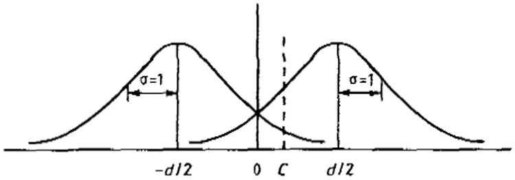
Distribution of filter outputs when s₂ is present (left) and when s₁ is present (right plotted against the tiller output. C, decision criterion; d, separation of means of the two distributions in units of their common standard deviation.

$$P(\text{TP})=\frac{1}{{(2\pi )}^{1/2}}{\int }_C^{\infty }exp\{-\frac{1}{2}{[z-(d/2)]}^2\}\mathrm{d}z=\frac{1}{{(2\pi )}^{1/2}}{\int }_{C-(d/2)}^{\infty }exp(-z^2/2)\mathrm{d}z$$ (5)

and his false positive rate P(fp)will be

$$P(\text{FP})=\frac{1}{{(2\pi )}^{1/2}}{\int }_{C+(d/2)}^{\infty }exp(-z^2/2)\mathrm{d}z$$ (6)

By varying the cut off level the resulting P(tp) and P(fp) levels will trace out the so called receiver operating characteristic (roc) curve (Green and Swets 1966, Swets and Pickett 1982). In the context of signal detection in additive Gaussian noise the snr is now seen to serve as a limit on the error integrals that determine performance.

We shall consider a simple example of detecting a signal in the presence of a white noise background. First, for x-ray imaging consider the detection of a pill box signal s₁ with incremental height ΔN counts per unit area above the background signal s₂ with N counts per unit area. The pill box profile h₀(r) is

$$\begin{array}{c}{h}_0(r)=\text{circle}(r/r_0)\\ r={(x^2+y^2)}^{1/2}\end{array}$$

The circle function is unity within a circle of radius r₀ and zero outside. In the Fourier domain the signal function becomes

$$\mathrm{\Delta }S=\mathrm{\Delta }N(\pi r_0^2)H_0(f)$$

where

$$f^2=f_x^2+f_y^2$$

and

$$(\pi r_0^2)H_0(f)\stackrel{\text{FT}}{\leftrightarrow }{h}_0(r)$$

$H_0^2(f)$ is the Airy disc function (Goodman 1968), normalised such that

$$2\pi {\int }_0^{\infty }{H}_0^2(f)f\mathrm{d}f=1/(\pi r_0^2)$$

The noise power spectral density for an uncorrelated Poisson-distributed photon density N is independent of spatial frequency, i.e. white noise, at a level equal to N. Then equation (4) gives trivially

$$\text{SNR}=\mathrm{\Delta }N{a}_0/{(N{a}_0)}^{1/2}=C^{\prime }{(N{a}_0)}^{1/2}$$

where

$$C^{\prime }=\mathrm{\Delta }N/N{a}_0=\pi r_0^2$$ (7)

This can be recognised as the snr used by Rose (1948) and Schade (1964).

In the 2D nmr case the signal is in volts per unit area, ΔV(x, y), proportional to the 2D density of spins, Δρ₂(x, y), and we have from Appendix 5

$$W=4kT{R}_{\mathrm{e}}\mathrm{\Delta }{f}_{\mathrm{t}}F/XY$$

Here k is Boltzmann's constant, T is the absolute temperature, R_e is the effective resistance of the receiving system (including the patient), Δf_t is the bandwidth of the communications receiver and F is the noise figure of the front end amplifier. The product of the overall dimensions X and Y is the total area over which signal is collected. Then the snr is simply

$$\text{SNR}=\mathrm{\Delta }{V}_2{(a_0)}^{1/2}{(XY)}^{1/2}/{(4kT{R}_{\mathrm{e}}\mathrm{\Delta }{f}_{\mathrm{t}}F)}^{1/2}$$ (8)

In principle there is photon noise in a communication channel and additive thermal noise in a radiation detection channel (Macovski 1983). The thermal noise energy during a temporal measurement interval 1/Δf_t is 4kT = 0.1 eV at laboratory and body temperatures. This is negligible compared with x-ray energies of 10⁴–10⁵ eV (frequencies of 10¹⁹–10²⁰ Hz) and the photon granularity is the dominating noise. In communication systems working in the low megahertz range the photon energy is 10⁻⁸–10⁻⁹ eV, there are very large numbers of quanta in detectable signals and the thermal noise in the detection stage dominates the very smooth granularity of the photons. Additional considerations for nmr imaging are given in Appendix 5.

If we take the signal s₁ in the example above to have a Gaussian profile h(x, y) with rms radius σ₀ and height ΔN, and take the background s₂ to be a uniform level of N counts per unit area (figure 2)

Figure 2.

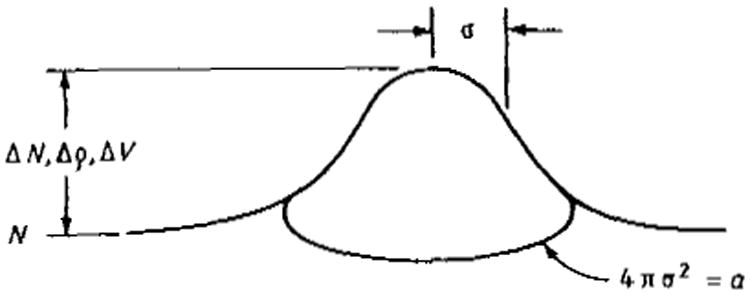
Low contrast Gaussian signals ΔN, Δρ and ΔV above background level N (or ρ or V). RMS radius equals σ. (See also notations used in table 2.)

$$\begin{array}{l}{s}_1=\mathrm{\Delta }Nh({\sigma }_0)+N\hfill \\ s_2=N=W\hfill \\ h({\sigma }_0)=exp[-(x^2+y^2)/2{\sigma }_0^2]\hfill \end{array}$$

then we have immediately from substitution into equation (3) or (4)

$${\text{SNR}}_{\text{qi}}={\text{SNR}}_{\mathrm{i}}=(C^{\prime }/2){(N{a}_0)}^{1/2}$$ (9)

where $a_0=4\pi {\sigma }_0^2$ and C′ = ΔN/N. The Gaussian weighting has reduced the form of the snr by a factor of two.

3. The snr(f) spectrum and the concept of the aperture

In practice, the signal in equations (1)–(4) will have experienced a macro-area transfer characteristic, from the input exposure axis to the output film density or detector current axis for example, with slope G, and a micro-area transfer function, the modulation transfer function mtf(f), yielding

$${\text{SNR}}_{\mathrm{i}}^2=\int \mathrm{d}f\frac{{[\mathrm{\Delta }S(f)]}^2{G}^2{\text{MTF}}^2(f)}{W(f)}$$ (10)

In conventional radiography, for example, W may be the spectrum of density fluctuations and then G is the product of lg(e) and the photographic gamma. For photon noise limited images the signal ΔS is frequently expressed as a contrast, i.e. in relative or logarithmic units (proportional to the attenuation coefficient for low contrasts). Then the quotient of the properly normalised G², mtf² and W is identified as the equivalent number of input quanta or noise equivalent quanta (neq) (Dainty and Shaw 1974) per unit area that, for an ideal imaging system, would give the same snr as the real exposure quanta degraded in information content by the actual imaging system (Shaw 1978, Sandrik and Wagner 1982)

$$\text{NEQ}(f)=G^2{\text{MTF}}^2(f)/W(f)$$ (11)

The fluctuations in detection system amplification and recording responsible for the degradation in large area information content have been studied by Swank (1973), Dick and Motz (1981) and Chan and Doi (1984); correlations in these mechanisms and their effect on higher frequency information content have been analysed by Metz and Vyborny (1983) and Shaw and Van Metier (1984). In images reconstructed from 2D line integral projections (computed tomography, ct) the 2D geometry provides an additional factor πf to the numerator of equation (11) (Hanson 1979a, Wagner et al 1979). (The approach of treating the signal and noise frequency channel by frequency channel is only strictly valid in the limit of low contrast signals where the noise is effectively additive and Gaussian. For true Poisson-distributed signals the noise is essentially multiplicative, the noise or fluctuations are correlated in the frequency domain (Metz 1969) and our straightforward formulation is no longer rigorous.)

The NEQ level is interpreted as the density of quanta the image is ‘worth’ based on the measurements G, mtf and W. The image is made for the ‘price’ of Q exposure quanta incident on the detector, but the measurements always show that it is worth fewer quanta because of the incomplete detection and the additional fluctuations beyond the input photon noise that show up in the output of the photon detection system. An example neq(f) spectrum from a second generation ct scanner operating in the normal head mode is given in figure 3 (Wagner et al 1979). In this example from a projection reconstruction system the low frequency value or worth is about 2 × 10⁸ quanta/cm along the projections, or perimeter of the scanned object. At higher frequencies, or on a finer scale, the image is usually worth less quanta than the neq(0) level. In this example the image at 3 cycles/cm is only worth half the number of quanta that it is worth near 0 cycles/cm, and it is worthless beyond about 6 cycles/cm. This approach is not a model; it is simply a scaling of the output noise W back to the input or exposure axis through the system transfer characteristic G mtf and the interpretation of the scaled fluctuations in terms of equivalent counts (Shaw 1978, Sandrik and Wagner 1982).

Figure 3.

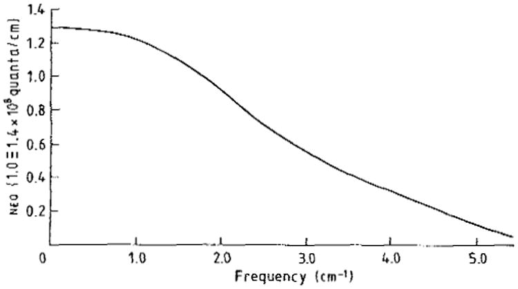
neq(f) spectrum for second generation ct system.

When only the low frequency neq level is of interest we write neq(0) or simply neq, which ignores the frequency dependence of W(f) and mtf(f). The closeness of the image neq level to the actual level Q of radiation impinging upon the detectors in 2D ct was used by Wagner et al (1979) to argue against the further pursuit of ‘low dose’ reconstruction algorithms; the detective quantum efficiency neq/Q (Shaw 1978) was comparable with the detectors' absorption efficiency. That meant that most of the low frequency information in the absorbed radiation showed up in the images produced by filtered backprojection. Hanson (1979a, 1980a) gave theoretical arguments for the optimality or efficiency of 2D filtered backprojection for large objects. His arguments can be restated and extended to 2D and 3D filtered backprojection independent of object size (as long as discrete effects can be neglected) as follows. The reconstructed image is rewhitened using the filter W^−1/2, where W is the appropriate noise power spectrum (Appendices 3 and 4); the snr in the whitened image is recognised as the snr in the original projections—it is, of course, the snr for the ideal observer discussed above. This snr corresponds to efficient signal estimation, i.e. achieving the minimum variance given by the Cramer-Rao bound (demonstrated in Appendix 2).

For thermal noise limited images a spatial frequency dependent noise equivalent temperature, noise equivalent resistance, or noise equivalent resistance–temperature product can be defined by analogy with the noise equivalent quanta concept. The choice will probably require a convention such as the specification of one or two of the parameters in the product TR_eΔf_t of equations (8) and (A45). Whereas the more quanta the better in photon limited imaging, the greater the resistance and temperature the worse in thermal limited imaging. This means that the noise equivalent thermal quantity will increase with spatial frequency, instead of decreasing as in the neq case.

Dainty and Shaw (1974) and Shaw (1978) have discussed the connections between the neq approach and the information theory of Shannon (1949). Shannon presented a precise measure of information (or the ‘state of disorder of knowledge’) which is similar to the measure of entropy (or state of molecular disorder) in statistical thermodynamics. He derived a result, now quite well known, for the information capacity of a communications channel. This result is proportional to the logarithm of the ratio of signal ‘power’ to noise ‘power’ in that channel. In the small signal limit the logarithmic measure is simply proportional to the snr² in the channel (Shaw 1963, Wagner et al 1979), here written as

$$\mathrm{\Delta }f{G}^2{\text{MTF}}^2(f)/W(f)\to \mathrm{d}f\text{NEQ}(f)$$

We see that the neq(f) approach and the Shannon channel approach lead to the same measure (Shaw 1963). (Shaw (1978) points out that Shannon's approach to the quantification of information in noisy communications channels is actually more general than the thermodynamics it resembles since it is applicable to problems involving any kind of uncertainty.) The ideal observer snr² is just an integral over the neq(f) spectrum—determined by the system detection hardware—weighted by the spectrum of a difference signal—corresponding to the observer's task (equation 10):

$${\text{SNR}}_{\mathrm{i}}^2=\int \mathrm{d}f{|\mathrm{\Delta }S(f)|}^2\text{NEQ}(f)$$ (12)

This equation, together with equation (11), demonstrates the fundamental equivalence of the statistical decision theoretic approach to snr, the information theoretic approach of Shannon and the spatial frequency spectrum of noise equivalent quanta of Shaw.

An important contribution to this kind of analysis has recently been made by Hanson (1983) who pointed out that several classes of image mensuration tasks based on edge detection give rise to snr² that are obtained by carrying out integrals over neq(f) weighted by powers of spatial frequency. The optimal detector in those cases can be recognised as a Laplacian derivative or higher order gradient matched filter (Andrews 1970). This means that the mid-frequency content of the neq spectrum takes on much greater importance than the low frequency content for such higher order tasks. In the case of the Rayleigh discrimination task, for example, where the observer must determine whether one star (lesion) or two are present (or measure the binary lesion separation) the snr² for small separations is proportional to the integral over the neq spectrum weighted by the fourth power of the spatial frequency along the discrimination axis. It is therefore quite sensitive to improvements (or degradations) in the mid-frequency neq performance.

Integrals over the snr²(f) spectrum play an inportant role in the analysis of imaging systems. We therefore define the normalised integral over this spectrum as the inverse of an effective length (or area) a_AP in one (or two) dimensions (according to the dimensionality of the integral)

$$a_{\text{AP}}^{-1}=\int \mathrm{d}f\text{NEQ}(f)/\text{NEQ}(0)$$ (13)

We shall see that this quantity is the fundamental measure of ‘resolution’ in a noise limited imaging system and therefore we dignify it with the name ‘the system aperture’. It is similar only in form to the measure of sharpness used by Schade (1964); the latter measure does not include the fundamental limits to snr due to coupling of the signal to additional background noise by the correct apperture (see next section). Integrals for the system aperture were carried out by Sandrik and Wagner (1982) in the application to screen–film systems yielding values for the aperture areas corresponding to lengths ranging from 0.1 to 0.3 mm. These values based on the neq(f) spectrum are about half the values obtained using the Schade equivalent aperture based only on the integral of the system mtf² (Wagner 1977). They are smaller because they correspond to the broader (sharper) effective mtf that results from the noise whitening implied in equations (4) and (11).

The system aperture for 2D ct was found (Wagner et al 1979) to be independent of the ct algorithm, as long as the algorithmic contribution to the mtf, mtf_alg, is non-zero at frequencies at which the non-algorithmic or hardware contribution to the mtf, mtf_AP, is non-zero, and to be expressible as

$$a_{\text{AP}}^{-1}\Rightarrow d_{\text{AP}}^{-1}={\int }_{-\infty }^{\infty }\mathrm{d}f\frac{{\text{MTF}}_{\text{total}}^2(f)}{{\text{MTF}}_{\text{alg}}^2(f)}$$ (14)

However

$${\text{MTF}}_{\text{total}}^2={\text{MTF}}_{\text{alg}}^2{\text{MTF}}_{\text{AP}}^2$$

therefore

$$d_{\text{AP}}^{-1}={\int }_{-\infty }^{\infty }\mathrm{d}f{\text{MTF}}_{\text{AP}}^2(f)$$

This results because the blurring effects of the ct algorithm contribute equally to the neq numerator through the total system ${\text{MTF}}_{\text{total}}^2$ and the denominator through the noise power spectrum W (Appendix 4), and cancel. Equation (13) is the general form for the interpretation of a system aperture; its dimensionality will depend on the imaging modality. Equation (14) became a ID integral since in ct the fundamental aperture is along the projection; the dimension along the axial direction is integrated out in the 2D analysis. Values for the aperture length ranged around 1 mm for late 1970s ct systems, the example in figure 3 giving about 1.6 mm.

The system aperture is an essential concept in the unified view. We shall presently see that it corresponds to a region over which signal counts are irretrievably coupled to background noise counts by those contributors to system blur which do not also blur the noise. A list of system apertures for various modalities is therefore given in table 1. We often refer to the system aperture as the terminal blur since it is induced by limitations in detection system hardware and cannot be corrected for by image processing, except in the non-physical limit of a noise free image source and detector.

Table 1.

The aperture or the terminal blur for various modalities.

Modality	System aperture
Radiology	Focal spot and portion of screen (neq bandwidth)
ct, dr	Focal spot and detector aperture (sampling greatly complicates)
rn	Collimator, detector
nmr	1/T2
	Field inhomogeneity
	Chemical shift

The approach to defining the neq(f) spectrum described above may be generalised to definitions appropriate to both linear and logarithmic detection schemes in 2D and 3D using results of the appendices of this paper. Grossman et al (1984) have given measured neqs for (linear, 2D) gamma camera systems neglecting mtf effects, but nothing has yet been reported along these directions for 3D systems.

In practice NEQ is also a function of the beam energy (Tapiovaara and Wagner 1984—discusses limitations of this concept in the context of iodine imaging) and exposure level (Wagner 1983, Bunch et al 1984). A considerable measurement effort may be required to adequately characterise it, but a rigorous specification of dynamic range in the snr sense then emerges.

The quantity in coherent ultrasound B-scanning analogous to neq is the density of coherent speckle spots over the image. The image speckles are the samplers of backscattered ultrasound signal just as detected photons are the samplers of x-ray attenuation signal. The average size of the speckle is specified in terms of its correlation length and this determines the density of spots. Since the correlation cell is comparable with a resolution cell (several wavelengths, of the order of 1 mm) the number of speckle spots in an ultrasound image is generally small enough to be counted by inspection and therefore detectable ultrasound contrasts are usually so large as to require a logarithmic scale (dB) for their specification. A quantitative analysis has been given by Wagner et al (1983a, b, c) and Smith et al (1983) for some special cases which are amenable to straightforward analysis, but much work remains for a general treatment.

4. The aperture and snr degradation

As an example of the aperture's role consider the Gaussian signal of the last section degraded by an aperture, e.g. x-ray tube focal spot, with transfer function

$$\text{MTF}(f)=H({\sigma }_{\text{AP}})=exp(-2{\pi }^2{\sigma }_{\text{AP}}^2{f}^2)$$ (15)

(We ignore the details of the geometrical scaling of this aperture and that of the image receptor to the object plane of interest; this is treated by Wagner 1977). Straightforward substitution of equation (15) into equation (10) yields

$${\text{SNR}}_{\mathrm{i}}=\frac{C^{\prime }}{2}{N}^{1/2}\frac{a_0}{{(a_0+a_{\text{AP}})}^{1/2}}=\frac{C^{\prime }}{2}{N}^{1/2}\frac{a_0^{1/2}}{{[1+(a_{\text{AP}}/a_0)]}^{1/2}}$$ (16)

where the power spectrum is again equal to N, independent of frequency, as in equation (7), since we define the system aperture as a blur function which does not correlate, or colour, the noise. As with other Gaussian functions we have $a_{\text{AP}}=4\pi {\sigma }_{\text{AP}}^2$ following the notation of equation (9). An interesting and fundamental interpretation of this result comes from comparing it with the snr for signal detection in the presence of scatter. Suppose we recalculate (Rose 1948) the snr above for the case

$$\begin{array}{c}{s}_1=P+S+\mathrm{\Delta }P{h}_0({\sigma }_0)\\ s_2=P+S\end{array}$$

where P represents the primary fluence and S the scatter fluence. It is straightforward to obtain for that case (Wagner et al 1980)

$${\text{SNR}}_{5\mathrm{c}}=\frac{(\mathrm{\Delta }P)a_0}{{[(P+S)a_0]}^{1/2}}=C^{\prime }\frac{P^{12}{a}_0^{1/2}}{{[1+(S/P)]}^{1/2}}$$ (17)

where the contrast C′ is ΔP/P = Δμx, i.e. the line integral of the attenuation coefficient difference between signal and background, essentially as before. Now we see that the role of the aperture in the snr of equation (16) is the same as the role played by the scatter term in equation (17), i.e. the aperture degrades snr by coupling signal to additional background noise in the way that the presence of scatter degrades snr by coupling signal to additional background noise counts. We shall return to this concept later in this paper.

The aperture functions chosen for the examples in this paper are taken to have Gaussian profiles to simplify the interpretation and discussion of results. The concept of the aperture is fundamental, however, and depends in no way on the actual shape of the function. For example, equation (12) is independent of the mtf profiles. Non-Gaussian apertures do not cascade by a simple quadrature sum, but they still represent the terminal image degrading mechanism of the coupling of noise to signal. The calculation of this degradation is no longer trivial, but is still straightforward following equations (10)–(12).

Finally, we point out that the aliasing that results from undersampling in a digital system degrades the aperture in a signal dependent way and is therefore difficult to treat generally. Developments in this direction have been made by Hanson (1979b) and Lissak Giger (1985).

We will be in a position to carry out the above analysis for any data acquisition modality once we have derived the noise power spectrum (nps) associated with the geometry and method of data acquisition. In Appendix 3, therefore, we derive the NPS for imaging using planar integrals in 3D; there the 3D volume is divided into planar slices (figures 4 and 5) and the signals are summed over the slice or cut, i.e. planar integrals analogous to the line integrals in conventional ct. The direction of the planes (or their normal vectors) is then varied over the surface of a sphere, analogous to the rotation of angle in ct. We shall find then that in images reconstructed by filtered backprojection the nps is proportional to f², where f is the radial spatial frequency.

Figure 4.

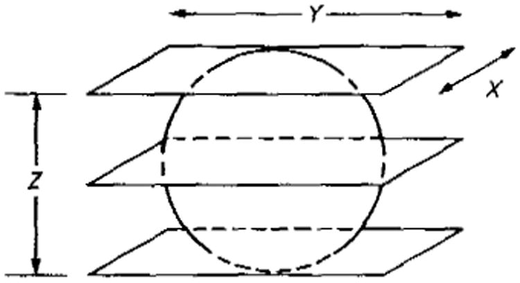
Geometry for planar integrals in 3D planar projection-reconstruction imaging. In practice there are many planes, more closely spaced. (See also figure 5). The diameter is D.

Figure 5.

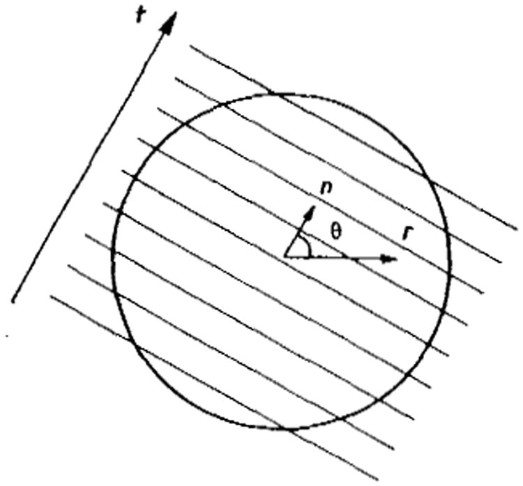
Geometry for calculations in Appendices 3 and 4.

In Appendix 4 the nps for imaging using 2D positron emission tomography is derived. The data collection is essentially by means of line integrals in the manner of conventional 2D ct. The nps from filtered backprojection is then proportional to f, the radial spatial frequency, just as in ct. 3D line integral techniques in which the integral direction is varied over all of 3D space have an nps proportional to f as in the 2D case.

In Appendix 5 the nps for 2D data acquisition in the Fourier domain is derived, with emphasis on the application to nmr imaging. We shall see that 2D Fourier techniques yield essentially a white noise spectrum or a low pass spectrum if the image is smoothed. The absolute level or normalisation of these nps depends on the variance in the measurements or integrated detected signals.

The next step is to use these nps in the expressions above for ${\text{SNR}}_{\text{qi}}^2$ and ${\text{SNR}}_{\mathrm{i}}^2$. The results for all of the modalities are given in table 2, columns 3 and 4, and 3 and 5 for the simplified cases in which the object shape, algorithm blurring and system aperture have Gaussian profiles. In this case the integrals in equations (3), (4) and (10) yield particularly simple forms, as above in equation (16). In column 6 we let the algorithm blur go to zero for ${\text{SNR}}_{\text{qi}}^2$. Finally, the results for ${\text{SNR}}_{\text{qi}}^2$ can be differentiated with respect to the algorithm blurring parameter and the optimal parameter used to maximise ${\text{SNR}}_{\text{qi}}^2$. This result is given in column 7. (When the objects and apertures do not have Gaussian profiles, equation (10) must be used with the appropriate profile functions; a handy aperture interpretation of the results is then not so immediate.)

Table 2.

Noise power spectra and snr² for ten modalities, snr² -Ax (aperture factors).

Mode	Noise power spectrum, W(f)	A	Aperture factors		${\text{SNR}}_{\mathrm{q}\mathrm{i}}^2(a_{\text{alg}}\to 0)/{\text{SNR}}_{\mathrm{i}}^2$	${\text{SNR}}_{\mathrm{q}\mathrm{i}}^2(\text{optimal}{a}_{\text{alg}})/{\text{SNR}}_{\mathrm{i}}^2$
			For ${\text{SNR}}_{\mathrm{q}\mathrm{i}}^2$	For ${\text{SNR}}_{\mathrm{i}}^2$
2D projection radiography	${\text{NEQ}}_2^{-1}{\text{MTF}}_{\text{alg}}^2(f)$	(Δμt)2 neq2	${\left(\frac{a_0}{2}\right)}^2\frac{a_N}{a_i^2}$	${\left(\frac{a_0}{2}\right)}^2\frac{1}{a_0+a_{\text{AP}}}$	1	1
2D energy selective radiography	${\text{NEQ}}_i^{-1}{\text{MTF}}_{\text{alg}}^2(f)$	(Δt1)2{Σi[cof(μ1i)]2/neqi}−1	${\left(\frac{a_0}{2}\right)}^2\frac{a_N}{a_i^2}$	${\left(\frac{a_0}{2}\right)}^2\frac{1}{a_0+a_{\text{AP}}}$	1	1
2D ct x-rays	$(\pi f/{\text{NEQ}}_1){\text{MTF}}_{\text{alg}}^2(f)$	Δμ2neq1	${\left(\frac{a_0}{2}\right)}^2\frac{2}{\pi }\frac{a_N^{3/2}}{a_i^2}$	${\left(\frac{a_0}{2}\right)}^2\frac{1}{{(a_0+a_{\text{AP}})}^{1/2}}$	$\frac{2}{\pi }$	$\frac{3^{3/2}}{2\pi }$
2D pet	$\frac{{\rho }_{2}Dexp(+\mu D)}{\eta m}\pi f{\text{MTF}}_{\text{alg}}^2(f)$	$\frac{C^{2}m{\rho }_2\eta exp(-\mu D)}{D}$	${\left(\frac{a_0}{2}\right)}^2\frac{2}{\pi }\frac{a_N^{3/2}}{a_i^2}$	${\left(\frac{a_0}{2}\right)}^2\frac{1}{{(a_0+a_{\text{AP}})}^{1/2}}$	$\frac{2}{\pi }$	$\frac{3^{3/2}}{2\pi }$
2D ct, nmr	$\frac{4k{\mathit{\text{TR}}}_{\mathrm{e}}\mathrm{\Delta }fF}{mD}\pi f{\mathit{\text{MTF}}}_{\text{alg}}^2(f)$	$\frac{\mathrm{\Delta }{V}_2^{2}mD}{4k{\mathit{\text{TR}}}_{\mathrm{e}}\mathrm{\Delta }fF}$	${\left(\frac{a_0}{2}\right)}^2\frac{2}{\pi }\frac{a_N^{3/2}}{a_i^2}$	${\left(\frac{a_0}{2}\right)}^2\frac{1}{{(a_0+a_{\text{AP}})}^{1/2}}$	$\frac{2}{\pi }$	$\frac{3^{3/2}}{2\pi }$
2D ft, nmr	$\frac{4k{\mathit{\text{TR}}}_{\mathrm{e}}\mathrm{\Delta }fF}{XY}$	$\frac{\mathrm{\Delta }{V}_2^{2}mD}{4k{\mathit{\text{TR}}}_{\mathrm{e}}\mathrm{\Delta }fF}$	${\left(\frac{a_0}{2}\right)}^2\frac{a_N}{a_i^2}$	${\left(\frac{a_0}{2}\right)}^2\frac{1}{a_0+a_{\text{AP}}}$	1	1
3D ct, line integrals, γ rays	$\frac{{\rho }_{3}Dexp(+\mu D)}{\eta m}2f{\text{MTF}}_{\text{alg}}^2(f)$	$\frac{C^{2}m{\rho }_3\eta exp(-\mu D)}{D}$	${\left(\frac{a_0}{2}\right)}^3\frac{\pi }{4}\frac{a_N^2}{a_i^3}$	${\left(\frac{a_0}{2}\right)}^3\frac{1}{a_0+a_{\text{AP}}}$	$\frac{\pi }{4}$	$\frac{8\pi }{27}$
3D ct, planar integrals, γ rays	$\frac{{\rho }_3\mathit{\text{DL}}exp(+\mu D)}{\eta m}2\pi f^2{\text{MTF}}_{\text{alg}}^2(f)$	$\frac{C^{2}m{\rho }_3\eta exp(-\mu D)}{\mathit{\text{DL}}}$	${\left(\frac{a_0}{2}\right)}^3\frac{1}{3}\frac{a_N^{5/2}}{a_i^3}$	${\left(\frac{a_0}{2}\right)}^3\frac{1}{{(a_0+a_{\text{AP}})}^{1/2}}$	$\frac{1}{3}$	$\frac{5^{5/4}}{9}$
3D ct planar integrals, nmr	$\frac{4k{\mathit{\text{TR}}}_{\mathrm{e}}\mathrm{\Delta }fF}{mD}2\pi f^2{\text{MTF}}_{\text{alg}}^2(f)$	$\frac{\mathrm{\Delta }{V}_3^{2}mD}{4k{\mathit{\text{TR}}}_{\mathrm{e}}\mathrm{\Delta }fF}$	${\left(\frac{a_0}{2}\right)}^3\frac{1}{3}\frac{a_N^{5/2}}{a_i^3}$	${\left(\frac{a_0}{2}\right)}^3\frac{1}{{(a_0+a_{\text{AP}})}^{1/2}}$	$\frac{1}{3}$	$\frac{5^{5/4}}{9}$
3D ft, nmr	$\frac{4k{\mathit{\text{TR}}}_{\mathrm{e}}\mathrm{\Delta }fF}{XYZ}$	$\frac{\mathrm{\Delta }{V}_3^{2}XYZ}{4k{\mathit{\text{TR}}}_{\mathrm{e}}\mathrm{\Delta }fF}$	${\left(\frac{a_0}{2}\right)}^3\frac{a_N^{3/2}}{a_i^3}$	${\left(\frac{a_0}{2}\right)}^3\frac{1}{{(a_0+a_{\text{AP}})}^{3/2}}$	1	1

a₀, area of object = $4\pi {\sigma }_0^2$.

a_AP, system aperture = $4\pi {\sigma }_{\text{AP}}^2$.

a_alg, area of algorithm blur = $4\pi {\sigma }_{\text{alg}}^2$.

a_j, area of image = a₀ + a_alg + a_AP.

a_N, noise sampling area = a₀ + 2a_alg + a_AP.

neq₁, noise equivalent quanta in 1D i.e. along the periphery of cut in ct (zero frequency value).

neq₂, noise equivalent quanta in 2D i.e. in the plane of the image (zero frequency value).

neq_I, noise equivalent quanta in the plane of the image for the ith energy in energy selective imaging.

μ_1i, mass attenuation coefficient of iodine for the ith energy in energy selective imaging.

t₁, iodine signal (g cm⁻²).

Δ, determinant of the matrix formed by mass attenuation coefficients in energy selective imaging (see, for example, Riederer and Mistretta 1977).

cof(μ_1i), cofactor of μ_1i in above matrix.

η, collection efficiency in γ ray imaging.

C′, signal contrast = Δρ/ρ, ΔN/N etc.

ρ₂ and ρ₃, 2D and 3D densities of γ radioactivity.

m, number of views.

ΔV₂ and ΔV₃, lesion signal excess in 2D and 3D nmr (volts per unit area or per unit volume).

4kTR_eΔf, thermal noise of effective resistance R_e with detection bandwidth Δf_r.

F, noise figure for electronics.

X, Y, Z, the three linear dimensions of the subject imaged.

D, subject diameter.

5. Discussion

There are only five fundamentally different geometrical modes of data acquisition considered in table 2: 2D direct measurement (in the coordinate or the Fourier domain); 3D direct measurement (Fourier domain); 2D line integral or projection measurement; 3D planar integral projections; and 3D line integral projections. Therefore columns 4 and 5 of table 2 for the aperture factors show only five different forms. Each form could have many practical realisations, however, both at present and in the future. We have chosen a total of ten realisations that are representative of the principal current applications.

Comparison of the various forms for the snr² in table 2 can be very instructive, as we shall presently see. Care must be taken in comparing them literally, however, since each snr² is for the particular signal quantity measured by the modality specified. For projection radiography, this is the line integral of the difference signal in attenuation coefficient ∫Δμ dl; for energy selective imaging, the integral of difference signal in iodine thickness, ∫ dt₁, or the thickness of another isolated material. For ct, it is the spatial distribution of the difference in attenuation coefficient μ in the case of x-rays, the difference in the 2D or 3D distribution of radioactivity ρ₂ or ρ₃ in the case of γ rays and the difference in the 2D or 3D density of proton spin density V₂ or V₃ in the case of nmr. The physical origin of these signals and their differences are specialised questions which we do not treat here; we will concentrate on the interaction of the measurement of these quantities and the propagation of the noise in their measurement. The interesting questions of optimising the contribution to the snr of the detected difference signal as a function of signal energy for photons (Oosterkamp 1961, Motz and Danos 1978) and pulse sequence for nmr (Edelstein et al 1983) are essential matters which are addressed elsewhere.

5.1. Resolution

The snrs of table 2 for the task of elementary signal detection are all reducible to an ideal observer contrast–diameter–exposure function of the form

$$C^2{d}^{n}Q=\text{constant}$$ (18)

for the case of a₀ → 0 or a₀ → ∞. Here C is the signal contrast, Q refers either to exposure quanta, noise equivalent quanta, or image exposure time and d refers to the diameter of the lesion to be detected and is proportional to $a_0^{1/2}$. The existence of such power laws for imaging systems is well known but the power cited for n is frequently incorrect or at least oversimplified. In table 3 we give the results we obtain for n using table 2 directly. ‘Large diameter’ and ‘small diameter’ regimes are defined with respect to the size of the system aperture, e.g. ‘large’ means much greater than the system aperture, etc. We see first of all the general result that for imaging in 2D and 3D the exposure or imaging time t depends on the inverse 4th and 6th powers of lesion diameter respectively (Barrett and Swindell 1981) for small diameter lesions. There is always a large diameter regime in which the dependence is not so severe.

Table 3.

Results for n using table 2. The snrs of table 2 are reducible to the form C²Qdⁿ = constant.

Modality	Large d	Small d
Photog./proj. imaging	2	4
2D ct—line integrals	3	4
2D ft	2	4
3D ct—planar integrals	5	6
3D ft	3	6

One application of this distinction is to the problem of ‘resolution’ in conventional and tomographic radiography. At any given state of technology it is always possible to move from the 4th or 6th power dependence to, say, a 3rd or 5th power dependence merely (!) for the cost of smaller sources and detector apertures, with noticeable improvement in detail resolution without an exposure cost. It is the effective density of detected quanta, or noise equivalent quanta, that must be kept constant and not the number of quanta per detector.

Another way of looking at this is to note that for lesion diameters in the neighbourhood of the aperture diameter there is a break between the lower power dependence and the higher power dependence (Wagner and Brown 1982). The break point is shifted towards smaller diameters as the aperture size is decreased. A region of small diameter detectability previously inaccessible has been made accessible simply by this shift and without changing the exposure. This has been taking place over the last five years in x-ray ct. It is also possible to achieve this in positron emission tomography (pet), although there is a fundamental limit to the improvement of resolution in pet scanning imposed by the range of the positron between emission and annihilation, approximately 1–5 mm depending on the isotope used (Fewell 1984).

A sharp reconstruction algorithm will be required to display the finer detail achievable by reducing the system aperture. This will increase the rms noise per displayed pixel, but this is an irrelevant parameter. The present analysis indicates that it is the density of neq and the size of the system aperture that are the principal determinants of lesion detectability. The argument is given in more detail by Wagner et al (1979) and Hanson (1979a). A demonstration that this is even the case for human observers is contained in the contrast–detail curves of Cohen and DiBianca (1979) and a presentation by Hanson (1980b).

The situation is somewhat more complicated for radionuclide imaging and single photon emission ct which are intrinsically dependent on hardware collimation. Analysis of the dose–resolution or exposure–resolution function for these systems requires a more detailed analysis such as that given by Wagner et al (1981).

Attempts to improve resolution in nmr imaging will run up against the fundamental nmr aperture limitations given in table 1, equivalent to the nmr line broadening. Consider the nmr line width as a cell size. Then the number of these cells across an image may indeed be increased, e.g. by increasing the field gradients (Gore 1982). This also requires increasing the detection bandwidth and therefore the detected noise (Appendix 5). The result is no change in the noise per cell, but a reduced signal per cell, with a requirement for more imaging time to maintain snr per cell. Other methods of obtaining finer resolution increase the imaging time explicitly, e.g. the additional scans required for additional resolution in the phase encoding direction in spin warp techniques (there is an effective aperture corresponding to the range of frequencies encoded in that direction). Thus, it is not possible in nmr imaging to improve resolution without increasing imaging time, all other things being held fixed (Redington 1982).

Finally, we emphasise that the power laws indicated in equation (18) and table 3 are for the simple lesion detection task. Frequently phantoms designed to measure the contrast–diameter or contrast–detail function in practice use rows of lesions instead of isolated lesions. The ideal observer functions for this task can be derived by considering tasks like Rayleigh discrimination discussed above. Then the value of n in table 3 for 2D imaging in the small diameter regime goes from 4 to 8 (Wagner et al 1985), and again we see the extreme sensitivity to the system aperture or the fall off of the NEQ spectrum for such discrimination tasks.

5.2. pr versus ft

We may compare the snrs for projection reconstruction (pr) or ct techniques against the snrs for Fourier transform (ft) techniques of data acquisition as given above under nmr imaging. In the 2D case the only factors that differ (in the limit of a_AP → 0) are the following

$$\text{FT}:Y/a_0^{1/2}\text{versus PR}:m$$ (19)

We see that for an object or lesion which is the size of the subject, i.e. $a_0^{1/2}=Y=X$, pr has an advantage equal to the number of views m. That is, each view contributes an independent estimate of the dc or large area signal in pr, while there is only one such estimate in an ft technique. For an object comparable with a pixel, $a_0^{1/2}$ = pixel dimension, the two become comparable if the number of views m is comparable with the number of pixels per view $Y/a_0^{1/2}$. In between, the algebra provides the correct relationship. (We refer here to the pixel dimension—the distance between reconstructed points—not as a length with a fundamental physical significance. It is not. It is merely a handy reference value here since typically m ≈ X/pixel dimension.) In § 6 on real observers we shall add to this discussion.

The argument just presented can be extended to the 3D case. Then we have the following differing factors

$$\text{FT}:YZ/a_0\text{versus PR}:m$$ (20)

and now we must compare the lession cross sectional area with the cross sectional area of the imaging volume. When their quotient is equal to the number of views, the pr and ft schemes are comparable for pixel sized lesions. For objects the size of the imaging volume, pr has an advantage equal to the number of views. Some of this will be cancelled by considerations raised below in § 6.

5.3. Time of flight pet

We may use the snrs of table 2 to determine the gain realisable from time of flight (tof) measurements in positron emission tomography (pet) scanning for the limit of perfect tof resolution. Perfect tof information would yield images whose snr per view would be the same as that of a conventional autoradiograph of the object, found from the first row of table 2. However, m views are used so the snr² should be increased m-fold. This can then be divided by the entry for snr² for 2D pet to give the ratio

$$\text{TOFPET gain limit}\to D{(a_0+a_{\text{AP CT}})}^{1/2}/(a_0+a_{\text{AP TOF}})$$ (21)

In the limit of $a_0^{1/2}\to D$, a lesion the size of the format, this gives unity, or no gain from tof information, which is obvious. In the other limit, a₀ → 0, the gain (for a_{AP CT} = a_{AP TOF}) is $D/a_{\text{AP}}^{1/2}$ which can be quite appreciable, currently of the order of 5–10. tof information additionally allows for great improvement in rejection of accidental coincidences (Ter-Pogossian et al 1982, Yamamoto et al 1982).

6. Performance of real observers

Practical measures of the performance of real observers include their true positive and false positive scores in yes/no type experiments or their per cent correct scores in two-alternative forced-choice experiments. These scores can be transformed into the snr of the real observer, snr_r, by the use of appropriate inverse error functions (Burgess et al 1981). The performance of the ideal observer in the same experiment can either be measured with a computer simulation or by calculating the snr from the imaging parameters. The ratio

$$\text{Observer efficiency}={\text{SNR}}_{\mathrm{r}}^2/{\text{SNR}}_{\mathrm{i}}^2$$ (22)

then expresses a statistical efficiency for the real observer and represents the fraction of the information in the image that he extracts in performing his task.

We may also write the definition of observer efficiency to include ${\text{SNR}}_{\text{qi}}^2$

$$\text{Observer efficiency}=({\text{SNR}}_{\mathrm{r}}^2/{\text{SNR}}_{\text{qi}}^2)({\text{SNR}}_{\text{qi}}^2/{\text{SNR}}_{\mathrm{i}}^2)\to (0.5\pm 0.2)(\text{observer}-\text{reconstruction efficiency})$$ (23)

The first factor in this expression has been found by Burgess et al (1981, 1982a, b) to cluster about 50% for a wide range of observer detection and discrimination tasks, including signal location uncertainty (Burgess and Ghandeharian 1984), as long as there is sufficient contrast displayed in the image. Insufficient display contrast or window capability leaves the signal in competition with the internal noise sources of the observer and drives the efficiency to much lower values. (It is curious that an observer of white noise images who differentiates the image, but is otherwise ideal, will have a signal detection efficiency of 50%. It is possible that the human observer does some such dc suppression in these tasks.)

The second factor is a measure of the efficiency of the observer in coping with the correlations which may be present in the noise. We refer to it as the observer–reconstruction efficiency since, in practice, it is generally only appreciably different from unity for images that have been reconstructed from projections. Human observers are generally unable to deal optimally with the negative correlations in these images that result from the subtractions, or dc suppression, that are essential to algorithms required for reconstruction from projections but lead to this observer–reconstruction efficiency loss. (The inverse of the observer–reconstruction efficiency is referred to as the observer-reconstruction penalty—Wagner et al 1984). A list of theoretical estimates of these efficiencies is given in table 2, column 6. The values are upper limits found from using the appropriate noise power spectra in equations (1), (4) and (10) for the quasi-ideal and ideal observers respectively. In practice, it appears that the human observer–reconstruction efficiency is somewhat lower than these limits for the conventional ct case (Burgess et al 1982b).

The reader may note that the observer–reconstruction efficiency has been calculated for 3D imaging systems without passing through the step of determining the nature of the noise in any 2D presentation of the 3D information. This was not required since the observer is performing a lesion detection task in 3D. If he proceeds according to the quasi-ideal strategy (or the ideal strategy) he will use a weighting function corresponding to the expected lesion in 3D space and ignore (or use) the information in the noise correlations in the 3D data. This remains true even if he proceeds through a stack of 2D data. (The derivations of equations (1), (3) and (4) do not depend on the dimensionality of the problem, and they describe the optimal integration or averaging over the full dimensionality.)

The ideal observer beats the observer–reconstruction penalty by either using a complicated averaging scheme in testing the image for the presence of a lesion, or equivalently by (p)rewhitening or uncorrelating the image noise before testing for the lesion (or fitting a model to the image—Hanson 1984). A poor (but practical) man's version of a prewhitening filter, with respect to the ct negative noise correlations, can be achieved by means of gross image smoothing. Joseph and collaborators (Joseph 1977, 1978; Joseph et al 1980) have found that in ct this requires first expanding the data scale to maintain numerical precision and then using a low pass filter function with a very low frequency cut off.

The smallest value in table 2, column 6 occurs for 3D reconstruction from planar integrals. We therefore expect to see a re-opening of the question of optimal image smoothing for data acquired by that technique. In the context of this paper we define optimal smoothing as the use of a post detection algorithm blur a_alg which maximises ${\text{SNR}}_{\text{qi}}^2$ (table 2, column 7). Our analysis shows that optimal smoothing in 3D reconstructions from planar integrals can raise the efficiency factor from $\frac{1}{3}$ to greater than $\frac{2}{3}$ (5^5/4/9, table 2, columns 6 and 7); the corresponding optimal smoothing for 2D ct raises the factor from 2/π ≃ 0.6 to about 0.8 (3^3/2/2π)(Wagner et al 1979; table 2). That is, the relative effect is much greater in the 3D case. In practice, as just noted, we find that the real observer-reconstruction efficiency is somewhat lower than the ratio of ${\text{SNR}}_{\text{qi}}^2/{\text{SNR}}_{\mathrm{i}}^2$ calculated here (Burgess et al 1982b). We speculate again that this is due to the fact that the real observer does some image differentiation, or dc suppression. Intuition and straightforward calculations show that this will lower his efficiency for Gaussian and disc shaped lesions: these signals carry significant low frequency information where the reconstruction noise is ramp-like, ∼f or weaker, ∼f². The situation is unclear for discrimination tasks that require no low frequency information (Burgess 1984). (In the application to nmr imaging the considerations of this paragraph must be balanced against the results of equations (19) and (20).)

It appears that in conventional imaging the quasi-ideal observer snr can be used to fit results of a range of human observer performance studies on both analogue and digital systems. This requires that the square of a human visual transfer function be included in both numerator and denominator integrals of equation (3) and a term be added in the denominator to represent the observer's internal noise (Loo et al 1984, Lissak Giger 1985). The dependence of this internal noise on the parameters of the image is the subject of current investigations (Burgess 1984).

7. Non-Gaussian statistics

In principle, the above analysis is only rigorous for additive Gaussian noise. However, for photon images the multiplicative Poisson noise becomes additive Gaussian noise in the limit of low contrast imaging and so the above analysis applies in that limit. Wagner et al (1981) considered the high contrast case, including the Poisson statistics of x-rays and γ rays, in a study of the multiplex advantage of coded aperture imaging.

Wagner et al (1983c) and Smith et al (1983) applied the fundamentals of statistical decision theory from which the above analysis derives to the Rayleigh statistics that result from ultrasound B-scans of scattering phantoms. Wagner et al (1983a, b), extended this work to the more general case of Rician statistics. The results fall within the general framework given here, but additional considerations are required. These will not be treated here.

8. Exposure efficiency

Finally, some considerations of system efficiency and exposure optimisation are given by Wagner and Jennings (1979) and Jafroudi et al (1982), including effects of scatter (Wagner et al 1980) and beam energy (Motz and Danos 1978). These treatments involve the concept of detective quantum efficiency and the generalisation of this to exposure and dose efficiency. The efficiency concepts involve normalisation of the above ${\text{SNR}}_{\mathrm{i}}^2$ quantities by exposure quanta (Sandrik and Wagner 1982) or dose (Hanson 1979a). Determination of these efficiencies allows the distance between the performance of the actual system being evaluated and the physically ideal system to be determined.

9. Conclusions

The ideal observer snr derived from statistical decision theory leads to an absolute scale for image system performance evaluation. It requires measurement of the large area and micro-area transfer characteristics and the noise power spectrum at a given operating point as a function of spatial frequency. This information can then be used to see how far a given system falls short of optimal design, to compare designs and project possible improvements and to chart the optimisation procedure. Once the ideal observer ${\text{SNR}}_{\mathrm{i}}^2$ is known for a given set of detected image parameters, the performance of the real observer can be measured and specified against this limiting performance. This specification is given as a statistical efficiency. Currently we understand that this efficiency can be compartmentalised, with one compartment associated with the inability of the human observer to rewhiten reconstruction-filtered noise. We speculate that another compartment is associated with the tendency of the real observer to differentiate or suppress the dc level of the image.

Finally, we note that the commonly measured ‘pixel variance’ has not appeared in our analysis. It may frequently be useful as a normalisation check, but it has no predictive power for signal detectability. The variance in the individual detection measurements is required, however, and serves as the absolute normalisation of the noise power spectra derived here. All theoretical as well as measured quantities in this paper are required to be measured and specified on an absolute scale (for further discussion, see Sandrik and Wagner 1982, Sandrik et al 1982).

Appendix 1

The likelihood function approach

Consider two scenes which, in the absence of noise, would have Fourier decompositions S₁(f) and S₂(f), where f refers to 2D or 3D frequency coordinates. Let the noise variance within a given frequency channel df be W(f) df, the noise spectral content, and take the noise to be independent of the signal level and to be Gaussian distributed. Then, going to discrete coordinates and assuming independent frequency channels, the likelihood of obtaining a set of measurements F_f given the presence of S₁ is simply

$$L(\{S_{1f}\})=\prod _f{(2\pi W_f)}^{-1/2}exp[-{(F_f-S_{1f})}^2/2W_f]$$ (A1)

and similarly for S₂ (see note at end of Appendix 1). The noise in Poisson images is additive and Gaussian in the low contrast limit and so the Fourier components are indeed independent; however, away from this limit this condition breaks down (Metz 1969).

For the task of deciding from the measurements which of the two scenes is present we define a decision function

$${\gamma }_{12}=L(S_1)/L(S_2)=\prod _{f}exp\left(\frac{-{(F_f-S_{1f})}^2+{(F_f-S_{2f})}^2}{2W_f}\right)$$ (A2)

If S₁ and S₂ are equally likely and of equal significance, then the decision would favour S₁ or S₂ depending on whether γ₁₂ > 1 or γ₁₂ < 1. If this cut off value or criterion is varied a reciever operating characteristic curve (roc) will be generated (Green and Swets 1966). Any monotonic function of γ₁₂ may be used as a decision function, so for simplicity we select a quantity proportional to the logarithm of γ₁₂

$${\psi }_{12}=\sum _f[{(F_f-S_{2f})}^2-{(F_f-S_{1f})}^2]/2W_f=\sum _f[-2F_f(S_{2f}-S_{1f})+(S_{2f}^2-S_{1f}^2)]/2W_f$$ (A3)

and the decision criterion is, if ψ₁₂ > 0 then S₁, if ψ₁₂ < 0 then S₂. (Since the quadratic terms in this expression are constants independent of the data, the decision function may be realised by cross correlation of the data F_f with the expected filtered difference image (S_2f − S_1f)/W_f, i.e. Σ_f F_f(S_2f − S_1f)/W_f)

Now we must calculate the probability that the application of the decision function will result in a correct decision. Assume S₁ is present. Then the readings taken by the decision maker are

$$F_f=S_{1f}+n_f$$

where n_f is the noise in frequency channel f. Then

$${\psi }_{12}(S_1)=\sum _f[{(S_{2f}-S_{1f})}^2-2n_f(S_{2f}-S_{1f})]/2W_f$$ (A4)

The probability of a correct decision is the probability that ψ₁₂ is greater than 0. If n_f is Normal (0, W_f), then ψ₁₂ is Normal (μ_ψ, ${\sigma }_{\psi }^2$), where we have in the limit of a continuous image spectrum

$$\begin{array}{c}{\mu }_{\psi }^2={(\int \mathrm{d}f{[S_2(f)-S_1(f)]}^2/2W_f)}^2\\ {\sigma }_{\psi }^2=\int \mathrm{d}f{[S_2(f)-S_1(f)]}^2/W_f\end{array}$$ (A5)

The probability of a correct decision is therefore

$$P(\text{TP})=\frac{1}{{(2\pi )}^{1/2}}{\int }_C^{\infty }exp\{-\frac{1}{2}{[z-(d/2)]}^2\}\mathrm{d}z=\frac{1}{{(2\pi )}^{1/2}}{\int }_{C-d/2}^{\infty }exp(-z^2/2)\mathrm{d}z$$ (A6)

where d/2 = μ_ψ/σ_ψ and C is the criterion or cut off value, here equal to zero.

The relationship between the binary decision problem treated here and the problem of parameter estimation is discussed by Hanson (1983), who has also indicated the connection with least-squares methods and the minimum χ² approach to the more general problem of multiple parameter estimation (Hanson 1984).

(Note that, in general, the function F is complex. The notation of this and the following appendix applies rigorously to complex quantities if the convention

$$AB=\frac{1}{2}[A{B}^{\ast }+A^{\ast }B]$$

is observed.)

Appendix 2

The Cramer–Rao bound

The quasi-ideal observer of this paper, given the binary task of discriminating whether an image corresponds to scene S₁ or S₂, will proceed according to the likelihood function approach of Appendix 1, except for making the assumption that the noise is white, or of constant density in the frequency domain. He will then use the decision function of equation (A3), assuming W_f = constant. His task is seen to be equivalent to estimating the cross correlation

$$\overline{\theta }=\sum _f{\overline{F}}_f(S_{2f}-S_{1f})$$ (A7)

that is, the expected image data in frequency space F̄_f as seen through the window of the difference signal. It is possible to calculate the minimum variance for this estimation task using methods introduced by Fisher and Cramer (see, for example, Cramer 1946), as we now show.

The likelihood function L, or the probability of obtaining the measurements F_f given the true or expected values of the measurements F̄_f, is

$$L(\{F_f\})=\prod {(2\pi W_f)}^{-1/2}exp[-{(F_f-{\overline{F}}_f)}^2/2W_f]$$ (A8)

As before we are working in the low contrast limit where the variance in F_f is just the component of the noise power spectrum at the frequency f, W_f, and these components are independent. The log likelihood function is

$$\text{Ig}L=-\sum _f{(F_f-{\overline{F}}_f)}^2/2W_f+K$$ (A9)

where K refers to terms independent of the estimation procedure. The minimum variance of unbiased estimators of θ̄, θ̂ is found from the Cramer–Rao bound

$${\sigma }_{\widehat{\theta }}^2\ge 1/\overline{T^2}\text{where}T=\partial (lgL)/\partial \overline{\theta }$$ (A10)

Here

$$T=\frac{\partial (lgL)}{\partial (\sum \mathrm{\Delta }{S}_f{\overline{F}}_f)}=\frac{\sum [(F_f-{\overline{F}}_f)/W_f](\mathrm{\Delta }{S}_f)}{\sum (\mathrm{\Delta }{S}_f^2)}$$ (A11)

and

$$\mathrm{\Delta }{S}_f=S_{2f}-S_{1f}$$

In obtaining the last step we have made a functional decomposition of the form:

$$\mathit{\lambda }=\frac{\langle \mathit{a}.\mathit{\lambda }\rangle \mathit{a}}{\langle \mathit{a}.\mathit{a}\rangle }+\frac{\langle \mathit{b}.\mathit{\lambda }\rangle \mathit{b}}{\langle \mathit{b}.\mathit{b}\rangle }+\dots {\lambda }_i=\langle \mathit{\lambda }.\mathit{i}\rangle =\frac{\langle \mathit{a}.\mathit{\lambda }\rangle }{\langle \mathit{a}.\mathit{a}\rangle }\langle \mathit{a}.\mathit{i}\rangle +\dots$$

where 〈a . b〉 = 0, etc. This is an orthogonalisation along basis directions (functions) a, b, etc, where the coefficients are given by inner products 〈a . λ〉 = Σ_i a_iλ_i in terms of a different orthogonal basis identified by the directions i (e.g. the Fourier basis). Then the functional derivative is

$$\frac{\partial {\lambda }_i}{\partial \langle \mathit{a}.\mathit{\lambda }\rangle }=\frac{\langle \mathit{a}.\mathit{i}\rangle }{\langle \mathit{a}.\mathit{a}\rangle }$$ (A12)

or, in our case with i → f, λ → F̄ and a → ΔS

$$\frac{\partial {\overline{F}}_f}{\partial (\sum {\overline{F}}_f\mathrm{\Delta }{S}_f)}=\frac{\mathrm{\Delta }{S}_f}{{\sum }_f\mathrm{\Delta }{S}_f^2}$$ (A13)

Now since

$$\overline{{(F_f-{\overline{F}}_f)}^2}=W_f$$

we obtain, returning to continuous coordinates

$${\sigma }_{\widehat{\theta }}^2\ge {(\int \mathrm{\Delta }{S}^2(f)\mathrm{d}f)}^2{(\int \frac{\mathrm{\Delta }{S}^2(f)}{W(f)}\mathrm{d}f)}^{-1}$$ (A14)

from equation (A10). This can be identified with the Schwartz' inequality result of equation (4) in the text, since there

$${\sigma }_{\widehat{\theta }}^2=\int W(f)\mathrm{\Delta }{S}^2(f)\mathrm{d}f$$ (A15)

Equality is achieved in equation (A14) when: (i) W(f) is constant, i.e., the noise is white in which case the quasi-ideal observer is in fact ideal; or (ii) the prewhitening procedure and filtering described after equation (4) in the text is implemented, in which case equations (A7) and (A13) would be modified by setting

$${\overline{F}}_f\to {\overline{F}}_f/W_f^{1/2}\mathrm{\Delta }{S}_f\to \mathrm{\Delta }{S}_f/W_f^{1/2}$$

This leads to the ideal observer and ideal observer snr of this paper.

We have thus shown that the ideal observer achieves the minimum variance set by the Cramer–Rao bound. Such an observer, or estimator, is said to be efficient (Cramer 1946), or in current parlance 100% efficient. He uses all of the information in the sample required for the task. Examples of the application of the Cramer–Rao bound to ct imaging have been given by Tretiak (1978) and Hanson (1980a).

Appendix 3

Noise power spectrum for 3D PR from planar integrals

This appendix closely parallels that in a previous paper on ct information theory (Wagner et al 1979) where we studied 2D reconstruction from line integral projections. Here we study the case of 3D reconstruction from planar integral projections. We seek the relationship between the noise power spectrum W(f), assumed spherically symmetric, and the variance in the projection or integral measurements, as propagated through the software or algorithmic transfer function mtf_alg. First we derive an expression for mtf_alg, in terms of G(f), the Fourier transform of the convolution filter function g(t). A parallel argument yields an expression for W(f) as a function of G(f).

The geometry is presented in figure 5. The parallel lines represent parallel planes as in figure 4 of the text. The projections are planar integrals, or projections of planes, onto an axis with coordinates t; the direction of the projections is defined in terms of the unit vector n which is normal to the projections planes, or parallel to the t axis. A reconstructed point of interest is located by its positional vector r = (x, y, z); if this is considered as a polar vector then n has angular coordinates θ, φ, where θ is the polar angle, and φ is the azimuthal angle. The reconstructed quantity μ(r) may be written in terms of the projections p(t_k, n_j) at position t_k and projection direction n_j, and the convolution weighting function g(t)

$$\mu (\mathit{r})=\frac{a}{m}\sum _{j=1}^m\sum _{k=-\infty }^{\infty }p(t_k,{\mathit{n}}_j)g(\mathit{r}.{\mathit{n}}_j-t_k)$$ (A16)

where m is the number of views and a is the increment between projection planes. This is just the 3D generalisation of filtered backprojection. It is analysed in detail by Chiu et al (1980). In the limit of infinite samples and views this becomes

$$\begin{array}{l}\mu (\mathit{r})=\frac{1}{4\pi }{\int }_0^{4\pi }\mathrm{d}\mathrm{\Omega }{\int }_{-\infty }^{\infty }\mathrm{d}tp(t,\mathit{n})g(\mathit{r}.\mathit{n}-t)\hfill \\ \mathrm{d}\mathrm{\Omega }=\mathrm{d}(cos\theta )\mathrm{d}\phi \hfill \end{array}$$ (A17)

With circular symmetry the projections are independent of θ and φ and there is no loss of generality upon setting x = y = 0, and z = r

$$\mu (\mathit{r})=\frac{1}{4\pi }{\int }_0^{4\pi }\mathrm{d}\mathrm{\Omega }{\int }_{-\infty }^{\infty }\mathrm{d}tp(t)g(rcos\theta -t)=\frac{1}{4\pi }{\int }_0^{\pi }\mathrm{d}\theta sin\theta {\int }_0^{2\pi }\mathrm{d}\phi {\int }_{-\infty }^{\infty }\mathrm{d}fP(f)G(f)exp(2\pi \mathrm{i}frcos\theta )$$ (A18)

where the last step may be viewed either as deriving from the shift theorem or the convolution theorem of Fourier analysis. P(f) is the Fourier transform of p(t, n) = p(t) by the spherical symmetry. The integral over θ can be done immediately and is proportional to (sin x)/x = j₀(x), the spherical Bessel function of order zero

$$\mu (\mathit{r})=\pi {\int }_0^{\infty }{f}^2\mathrm{d}f(\frac{P(f)G(f)}{2\pi f^2})j_0(2\pi fr)$$ (A19)

which we have written in a form convenient for identification as the 3D Fourier transformation of a spherically symmetric function, i.e.

$$\mu (\mathit{r})={\mathcal{F}}_3^{-1}\left(\frac{P(f)G(f)}{2\pi f^2}\right)$$ (A20)

With a delta function input, the absolute value of the quantity in parentheses is the system total mtf

$${\text{MTF}}_{\text{total}}=\left|\frac{P(f)G(f)}{2\pi f^2}\right|$$ (A21)

which in turn is the product of algorithimic (software) and non-algorithmic (hardware aperture) contributions

$${\text{MTF}}_{\text{total}}={\text{MTF}}_{\text{alg}}{\text{MTF}}_{\text{AP}}$$ (A22)

The projection for a delta function input at the origin and an infinitesimal aperture function is equivalent to P(f)= 1, allowing us to identify

$${\text{MTF}}_{\text{alg}}=\left|\frac{G(f)}{2\pi f^2}\right|$$ (A23)

The noise power spectrum is obtained similarly. The autocovariance C of the reconstructed quantity μ is given by the expectation value

$$C(\mathit{r},0)\equiv C(\mathit{r})=\langle \delta \mu (\mathit{r})\delta \mu (0)\rangle$$ (A24)

where δμ is the deviation of μ from its mean value. Then if the measurements are uncorrelated with variance Σ²

$$\langle \delta p(t_k{\mathit{n}}_j)\delta p(t_{k^{\prime }},{\mathit{n}}_j)\rangle ={\sum }^2{\delta }_{k{k}^{\prime }}{\delta }_{j{j}^{\prime }}$$ (A25)

we obtain

$$C(\mathit{r})=\frac{{\sum }^2{a}^2}{m}\sum _{k,j}g(\mathit{r}.{\mathit{n}}_j-t_k)g(-t_k)$$ (A26)

or in the limit of continuous sampling

$$C(\mathit{r})=\frac{{\sum }^{2}a}{4\pi m}{\int }_0^{4\pi }\mathrm{d}\mathrm{\Omega }{\int }_{-\infty }^{\infty }\mathrm{d}tg(rcos\theta -t)g(-t)$$ (A27)

where

$$4\pi /m=\mathrm{\Delta }\mathrm{\Omega }\to \mathrm{d}\mathrm{\Omega }a=\mathrm{\Delta }t\to \mathrm{d}t$$ (A28)

Notice that

$$C(0)=\frac{{\sum }^{2}a}{m}{\int }_{-\infty }^{\infty }{g}^2(t)\mathrm{d}t={\sigma }_{\text{pixel}}^2$$

the pixel variance, which could have been derived using the result for the variance of a weighted mean. As above we may write

$$C(\mathit{r})=\frac{a{\sum }^2}{4\pi m}{\int }_0^{4\pi }\mathrm{d}\mathrm{\Omega }{\int }_{-\infty }^{\infty }\mathrm{d}f{|G(f)|}^{2}exp(2\pi \mathrm{i}frcos\theta )$$ (A29)

or

$$=\frac{a{\sum }^2}{m}{\mathcal{F}}_3^{-1}\left(\frac{{|G(f)|}^2}{2\pi f^2}\right)$$

Since the noise power spectrum is the ft of the autocovariance function we identify the product of aΣ²/m and the quantity within the parentheses as W(f), or in terms of mtf_alg

$$W(f)=({\sum }^{2}a/m)(2\pi f^2){\text{MTF}}_{\text{alg}}^2(f)$$ (A30)

Appendix 4

Noise power spectrum for 2D positron emission tomography

The noise power spectrum W(f) for this modality follows immediately from our treatment of 2D ct (Wagner et al 1979), or from the previous appendix for 3D ct. Here, W(f) is assumed to be circularly symmetric. For applications where this does not hold due to asymmetry toward the edge of the field, see Tanaka and Murayama (1982) and Hanson (1980c). The argument of Appendix 3 is essentially the same when carried out in 2D but the special function will be the circular Bessel function J₀ instead of the spherical Bessel function j₀. Equation (A27) becomes

$$C(\mathit{r})=\frac{a{\sum }^2}{4\pi m}{\int }_0^{\pi }\mathrm{d}\theta {\int }_{-\infty }^{\infty }g(rcos\theta -t)g(t)\mathrm{d}t$$ (A31)

and the notation is that of Appendix 3 or Wagner et al (1979). Alternative normalisations are possible; they make no difference when the result is given in terms of mtf_alg as done here. As above, using the convolution theorem:

$$C(\mathit{r})=\frac{a{\sum }^2}{4\pi m}{\int }_0^{\pi }\mathrm{d}\theta {\int }_{-\infty }^{\infty }\mathrm{d}f{|G(f)|}^{2}exp(2\pi \mathrm{i}frcos\theta )=\frac{a{\sum }^2}{m}{\mathcal{F}}_2^{-1}\left\{\frac{{|G(f)|}^2}{4\pi f}\right\}$$ (A32)

In this case we have

$${\text{MTF}}_{\text{alg}}=\left|\frac{G(f)}{2\pi f}\right|$$ (A33)

and so we can make the identification

$$W(f)=\frac{a{\sum }^2}{m}(\pi f){\text{MTF}}_{\text{alg}}^2(f)$$ (A34)

If the object is a cylindrical slab of diameter D and uniform 2D activity distribution ρ₂, and the attenuation coefficient μ is uniform over the slab, we require the variance per measurement of the line integral ∫ ρ₂ dl → ρ₂D

$${\sum }^2=var({\rho }_{2}D)$$ (A35)

In this derivation all chords of the slab are equal to D (i.e. near the centre of the circle), and therefore the photon attenuation is exp(−μl) exp[−μ(D − 1)] = exp(−μD), independent of l, the distance of the annihilation from the perimeter of the object. The variance may be obtained in terms of the detected counts per measurement ρ₂Daη exp(−μD), where η is the combined geometrical/quantum collection efficiency of the detection system, using var(bX) = b²var(X)

$${\sum }^2={[a^2{\eta }^{2}exp(-2\mu D)]}^{-1}[a\eta {\rho }_{2}Dexp(-\mu D)]={\rho }_{2}D/a\eta exp(-\mu D)$$ (A36)

We obtain finally

$$W(f)=\frac{{\rho }_{2}D}{m\eta exp(-\mu D)}(\pi f){\text{MTF}}_{\text{alg}}^2(f)$$ (A37)

Appendix 5

Noise power spectrum for 2D Fourier acquisition of nmr data

We shall first demonstrate that the intrinsic noise associated with the origin of the nmr signal is negligible in nmr imaging. Then we give the well known expression for thermal noise at the signal detection stage and consider its propagation through a typical nmr signal processing algorithm.

The nmr signal originates in a transition between two magnetic spin levels separated in energy by ΔE. The energy separation is proportional to the static field H

$$\mathrm{\Delta }E=h{f}_{\mathrm{t}}=h(\gamma /2\pi )H$$ (A38)

Here h is Planck's constant, f_t is the frequency of the nmr signal, and γ is the gyromagnetic ratio; for protons γ/2π is equal to 42.6 MHz T⁻¹. At 1 T and for kT in the body approximately equal to $\frac{1}{40}$ eV, the ratio n̄₁/n̄₂ of the mean populations of the two spin states is given by the Boltzmann factor

$$\frac{{\overline{n}}_1}{{\overline{n}}_2}=exp(\mathrm{\Delta }E/kT)\simeq 1+\mathrm{\Delta }E/kT=1.00000693$$ (A39)

The statistical broadening of the populations may be calculated by considering the total sample of N = n₁ + n₂ spins to play out a binomial process. The mean population of the low energy state will be Nθ, that of the high energy state N(1 − θ), with the binomial parameter θ very nearly $\frac{1}{2}$; both states will have variance ${\sigma }_{\mathrm{B}}^2=N\theta (1-\theta )$. For large populations the difference Δ = n₁ − n₂ = 2n₁ − N will be distributed very nearly Gaussian, $G(2{\overline{n}}_1-N,4{\sigma }_{\mathrm{B}}^2)$. Setting θ = (1 + ε)/2 we have for the probability density of Δ, p(Δ) = G[εN, N(1 − ε²)] with 2ε ≃ ΔE/kT.

At human body temperature there are approximately N = 6.69 × 10²² protons/cm³ in H₂O yielding the values in table 4 for the mean, standard deviation and coefficient of variation in the difference signal, ignoring saturation effects. This inherent noise in the nmr signal will not be appreciable for this order of the field strength unless the sample volume is smaller than the order of (0.01 mm)³.

Table 4.

Binomial parameters for nmr at I T.

Parameter	Formula	Sample volume
		1 cm3	1 mm3
Mean, μΔ	εN	2.2 × 1017	2.2 × 1014
Variance ${\sigma }_{\mathrm{\Delta }}^2$	N(1 – ε2) ∼ N	6.6 × 1022	6.6 × 1019
Coefficient of variation (σ/μ)Δ	1/εN1/2	1.2 × 10−6	3.8 × 10−5

The noise in nmr imaging therefore derives primarily from the thermal noise generated in the effective resistance R_e of the patient and the receiving coil (Hoult and Lauterbur 1979). The noise variance per measurement is then 4kTR_eΔf_t, where k is Boltzmann's constant, T is the absolute temperature, and Δf_t is the bandwidth of the receiver. The front end amplification will degrade this by its noise figure F to (4kTR_eΔf_t)F.

The most commonly used nmr imaging algorithm today is the discrete 2D Fourier transform. The nmr signal in the temporal domain encodes 1 D positional information in its temporal frequency representation; this frequency is scaled (equation A38) to a positional coordinate according to the strength and direction of the applied magnetic field gradient ∂H/∂x. A ‘pseudo-temporal’ domain is generated for encoding positional information in an orthogonal direction using a sequence of sinusoidally varying phase encodings to produce a Fourier representation in that direction (see for example Edelstein et al 1980).

For imaging in 2D we shall consider a 2D distribution of magnetism ρ₂(x, y), with the Fourier transform representation:

$$\begin{array}{c}{\rho }_2(x,y)=\sum _{f_x{f}_y}R(f_x,f_y)exp[-2\pi \mathrm{i}(f_{x}x+f_{y}y)]\mathrm{\Delta }{f}_x\mathrm{\Delta }{f}_y\\ R(f_x,f_y)=\sum _{xy}{\rho }_2(x,y)exp[2\pi \mathrm{i}(f_{x}x+f_{y}y)]\mathrm{\Delta }x\mathrm{\Delta }y\end{array}$$ (A40)

and with normalisations simplified to unity since linear frequencies f_x and f_y are used instead of the angular frequencies ω_x, ω_y. The autocorrelation between the image noise at points (0, 0) and (x, y), 〈δρ(x, y)δρ(0, 0)〉, is then related to the autocorrelation of the measurements in time and pseudo-time $\langle R(f_x,f_y)R(f_x^{\prime },f_y^{\prime })\rangle$ (so written because time is equivalent to spatial frequency) by the transformation

$$\langle \delta \rho (x,y)\delta \rho (0,0)\rangle =\sum _{f_x{f}_y}\sum _{f_x^{\prime }{f}_y^{\prime }}\langle R(f_x,f_y)R(f_x^{\prime },f_y^{\prime })\rangle exp[-2\pi \mathrm{i}(f_{x}x+f_{y}y)]\times \mathrm{\Delta }{f}_x\mathrm{\Delta }{f}_x^{\prime }\mathrm{\Delta }{f}_y\mathrm{\Delta }{f}_y^{\prime }$$ (A41)

Since the thermal noise is white or uncorrected we can write

$$\langle R(f_x,f_y)R(f_x^{\prime },f_y^{\prime })\rangle ={\delta }_{f_x{f}_x^{\prime }}{\delta }_{f_y{f}_y^{\prime }}(4kT{R}_{\mathrm{e}}\mathrm{\Delta }{f}_{\mathrm{t}})F$$ (A42)

and obtain immediately for the image noise autocorrelation

$$\langle \delta {\rho }_2(x,y)\delta {\rho }_2(0,0)\rangle =\sum _{f_x{f}_y}\left(\frac{(4kT{R}_{\mathrm{e}}\mathrm{\Delta }{f}_{\mathrm{t}})F}{XY}\right)exp[-2\pi \mathrm{i}(f_{x}x+f_{y}y)]\mathrm{\Delta }{f}_x\mathrm{\Delta }{f}_y$$ (A43)

where the spatial frequency resolution is Δf_x = 1/X, Δf_y = 1/Y when the region scanned has dimensions X and Y. We can now identify the noise power spectrum as

$$W(f)=\frac{(4kT{R}_{\mathrm{e}}\mathrm{\Delta }{f}_{\mathrm{t}})F}{XY}$$ (A44)

By the methods of the previous appendix we would have had for the nmr 2D ct case

$$W(f)=\frac{(4kT{R}_{\mathrm{e}}\mathrm{\Delta }{f}_{\mathrm{t}})F}{mD}\pi f{\text{MTF}}_{\text{alg}}^2(f)$$ (A45)

where D is the dimension along the projections (equal to X or Y for the squared circle).

Practical aspects of nmr image noise are discussed by Ortendahl et al (1984).

References

- Andrews HC. Computer Techniques in Image Processing. ch 4 New York: Academic; 1970. [Google Scholar]
- Barrett HH, Swindell W. Radiological Imaging: The Theory of Image Formation, Detection and Processing. Vol. 2. New York: Academic; 1981. [Google Scholar]
- Bunch PC, Shaw R, Van Metter RL. SPIE Proc vol 454: Medicine XII. Vol. 1984. Bellingham, WA: SPIE; p. 154. [Google Scholar]
- Burgess AE. SPIE Proc vol 454: Medicine XII. Bellingham, WA: SPIE; 1984. p. 18. [Google Scholar]
- Burgess AE, Ghandeharian H. J Opt Soc Am. 1984;Al:906. doi: 10.1364/josaa.1.000906. [DOI] [PubMed] [Google Scholar]
- Burgess AE, Jennings RJ, Wagner RF. J Appl Photogr Eng. 1982a;8:76. [Google Scholar]
- Burgess AE, Wagner RF, Jennings RJ. Proc Int Workshop on Physics and Engineering in Medical Imaging (Pacific Grove, CA) 1982. 1982b:99. IEEE Cat. No 82CH1751-7. [Google Scholar]
- Burgess AE, Wagner RF, Jennings RJ, Barlow HB. Science. 1981;214:93. doi: 10.1126/science.7280685. [DOI] [PubMed] [Google Scholar]
- Chan HP, Doi K. Med Phys. 1984;11:37. doi: 10.1118/1.595474. [DOI] [PubMed] [Google Scholar]
- Chiu MY, Barrett HH, Simpson RG. J Opt Soc Am. 1980;70:755. [Google Scholar]
- Cohen G, DiBianca FA. J Comput Assist Tomogr. 1979;3:189. doi: 10.1097/00004728-197904000-00008. [DOI] [PubMed] [Google Scholar]
- Cook CE, Bernfeld M. Radar Signals. New York: Academic; 1967. [Google Scholar]
- Cramer H. Mathematical Methods of Statistics. Princeton: Princeton University; 1946. p. 477. [Google Scholar]
- Dainty JC, Shaw R. Image Science. London: Academic; 1974. p. 156. [Google Scholar]
- Dick CE, Motz JW. Med Phys. 1981;8:337. doi: 10.1118/1.594836. [DOI] [PubMed] [Google Scholar]
- Edelstein WA, Bottomley PA, Hart HR, Smith LS. J Comput Assist Tomogr. 1983;7:391. doi: 10.1097/00004728-198306000-00001. [DOI] [PubMed] [Google Scholar]
- Edelstein WA, Hutchison IMS, Johnson G, Redpath T. Phys Med Biol. 1980;25:751. doi: 10.1088/0031-9155/25/4/017. [DOI] [PubMed] [Google Scholar]
- Fcwcll T R 1984 private communication
- Goodman JW. Introduction to Fourier Optics. San Francisco: McGraw-Hill; 1968. [Google Scholar]
- Gore JC. NMR Imaging: Proc Int Symp on Nuclear Magnetic Resonance Imaging. Winston-Salem, NC: Bowman Gray; 1982. p. l5. [Google Scholar]
- Green DM, Swets JA. Signal Detection Theory and Psychophysics. New York: Wiley; 1966. reprint 1974 (Huntingdon NY: Krieger) [Google Scholar]
- Grossman LW, Anderson MP, Jennings RJ, ICruger JB, Lukes SJ, Wagner RF, WaiT CP. SPIE Proc vol 454: Medicine XII. Bellingham, WA: SPIE; p. 1984.p. 215. [Google Scholar]
- Hanson KM. Med Phys. 1979a;6:441. doi: 10.1118/1.594534. [DOI] [PubMed] [Google Scholar]
- Hanson KM. SPIF Proc vol 173: Medicine VII. Bellingham, WA: SPIE; 1979b. p. 291. [Google Scholar]
- Hanson KM. J Comput Assist Tomogr. 1980a;4:361. doi: 10.1097/00004728-198006000-00012. [DOI] [PubMed] [Google Scholar]
- Hanson KM. Med Phys. 1980b;7:421. doi: 10.1118/1.594673. abstract G3. [DOI] [PubMed] [Google Scholar]
- Hanson KM. Med Phys. 1980c;1:421. abstract G4. [Google Scholar]
- Hanson KM. SPIE Proc vol 419: Medicine XI. Bellingham, WA: SPIE; 1983. p. 60. [Google Scholar]
- Hanson KM. SPIE Proc vol 454: Medicine XII. Bellingham, WA: SPIE; 1984. p. 9. [Google Scholar]
- Harris JL. J Opt Soc Am. 1964;54:606. [Google Scholar]
- Hoult DI, Lauterbur PC. J Magn Reson. 1979;34:425. [Google Scholar]
- Jafroudi H, Mumz EP, Bernstein H, Jennings RJ. SPIE Proc vol 347: Medicine X. Bellingham, WA: SPIE; 1982. p. 75. [Google Scholar]
- Joseph PM. SPIE Proc vol 127: Medicine VI. Bellingham, WA: SPIE; 1977. p. 43. [Google Scholar]
- Joseph PM. Opt Eng. 1977;17:396. [Google Scholar]
- Joseph PM, Hilal SK, Schulz RA, Kelcz F. Radiology. 1980;134:507. doi: 10.1148/radiology.134.2.7352241. [DOI] [PubMed] [Google Scholar]
- Judy PF, Swensson RG, Szulc M. Med Phys. 1981;8:13. doi: 10.1118/1.594903. [DOI] [PubMed] [Google Scholar]
- Kroger RA, Liu PY. IEEE Trans Med Imaging. 1982;MI-1:16. doi: 10.1109/TMI.1982.4307544. [DOI] [PubMed] [Google Scholar]
- Lissak Giger M, Doi K. Recent Developments in Digital Imaging, 1984 AAPM Annual Summer School. New York: American Institute of Physics; 1985. [Google Scholar]
- Loo L-N D, Doi K, Metz CE. Phy Med Biol. 1984;29:837. doi: 10.1088/0031-9155/29/7/007. [DOI] [PubMed] [Google Scholar]
- Macovski A. Medical Imaging Systems. Englewood Cliffs, NJ: Prentice-Hall; 1983. [Google Scholar]
- Metz CE. PhD Thesis University of Pennsylvania. Ann Arbor, Ml: University Microfilms; 1969. A Mathematical Investigation of Radioisotope Scan Image Processing. 70–16 186. [Google Scholar]
- Metz CE, Vyborny CJ. Phys Med Biol. 1983;28:547. doi: 10.1088/0031-9155/28/5/008. [DOI] [PubMed] [Google Scholar]
- Motz JW, Danos M. Med Phys. 1978;5:8. doi: 10.1118/1.594405. [DOI] [PubMed] [Google Scholar]
- North DO. Proc IEEE. 1963;51:1016. [Google Scholar]
- Oosterkamp WJ. Medicamundi. 1961;7:68. [PubMed] [Google Scholar]
- Ortendahl DA, Hylton NM, Kaufman L, Crooks LE. Mag Res Med. 1984;1:316. doi: 10.1002/mrm.1910010304. [DOI] [PubMed] [Google Scholar]
- Papoulis A. Probability Random Varables and Stochastic Processes. New York: McGraw-Hill; 1965. [Google Scholar]
- Redington RW. IEEE Trans Med Imaging. 1982;MI-1:230. doi: 10.1109/TMI.1982.4307588. [DOI] [PubMed] [Google Scholar]
- Riederer SJ, Mistretta CA. Med Phys. 1977;4:474. doi: 10.1118/1.594357. [DOI] [PubMed] [Google Scholar]
- Roetling PG, Trabka EA, Kinzly RE. J Opt Soc Am. 1968;58:342. [Google Scholar]
- Rose A. J Opt Soc Am. 1948;38:196. doi: 10.1364/josa.38.000196. [DOI] [PubMed] [Google Scholar]
- Sandrik JM, Wagner RF. Med Phys. 1982;9:540. doi: 10.1118/1.595099. [DOI] [PubMed] [Google Scholar]
- Sandrik JM, Wagner RF, Hanson KM. Appl Opt. 1982;21:3597. doi: 10.1364/AO.21.003597. [DOI] [PubMed] [Google Scholar]
- Schade OH. J SMPTE. 1964;73:81. [Google Scholar]
- Shaw R. J Photogr Sci. 1963;11:199. [Google Scholar]
- Shaw R. Rep Prog Phys. 1978;41:1103. [Google Scholar]
- Shaw R, Van Metter RL. SPIE Procr vol 454: Medicine XII. Bellingham, WA: SPIE; 1984. pp. 128–133. [Google Scholar]
- Shannon CE. Proc IRE. 1949;37:10. [Google Scholar]
- Smith SW, Wagner RF, Sandrik JM, Lopez H. IEEE Trans Sonics Ultrason. 1983;30:164. [Google Scholar]
- Swank RK. J Appl Phys. 44:1973. 4199. [Google Scholar]
- Swets JA, Pickett RM. Evaluation of Diagnostic Systems: Methods from Signal Detection Theory. New York: Academic; 1982. [Google Scholar]
- Tanaka E, Murayama H. Proc Int Workshop on Physics and Engineering in Medical Imaging (Pacific Grove, CA) 1982. 1982:158. IEEE Cat. No 82CH1751-7. [Google Scholar]
- Tapiovaara MJ, Wagner RF. SPIE Proc vol 454: Medicine XII. Vol. 1984. Bellingham, WA: SPIE; p. 52. [Google Scholar]
- Ter-Pogossian MM, Ficke DC, Yamamoto M, Hood JT. IEEE Trans Med Imaging. 1982;MI-1:179. doi: 10.1109/TMI.1982.4307570. [DOI] [PubMed] [Google Scholar]
- Thomas JB. An Introduction to Statistical Communication Theory. New York: Wiley; 1969. p. 212. [Google Scholar]
- Tretiak OJ. J Comput Assist Tomogr. 1978;2:477. doi: 10.1097/00004728-197809000-00019. [DOI] [PubMed] [Google Scholar]
- Wagner RF. Med Phys. 1977;4:279. doi: 10.1118/1.594362. [DOI] [PubMed] [Google Scholar]
- Wagner RF. Photogr Sci Eng. 1978;22:41. see also Photogr. Sci. Eng.22 336. [Google Scholar]
- Wagner RF. IEEE Trans Med Imaging. 1983;MI-2:105. [Google Scholar]
- Wagner RF, Barnes GT, Askins BS. Med Phys. 1980;7:13. doi: 10.1118/1.594773. [DOI] [PubMed] [Google Scholar]
- Wagner RF, Brown DG. IEEE Trans Med Imaging. 1982;MI-1:210. doi: 10.1109/TMI.1982.4307580. [DOI] [PubMed] [Google Scholar]
- Wagner RF, Brown DG, Burgess AE, Hanson KM. J Mag Res Med. 1984;1:76. doi: 10.1002/mrm.1910010109. [DOI] [PubMed] [Google Scholar]
- Wagner RF, Brown DG, Pastel MS. Med Phys. 1979;6:83. doi: 10.1118/1.594559. [DOI] [PubMed] [Google Scholar]
- Wagner RF, Brown DG, Metz CE. SPIE Proc vol 314: Conf on Digital Radiography. Bellingham, WA: SPIE; 1981. p. 72. [Google Scholar]
- Wagner RF, Brown DG, Smith SW. Ultrason Imaging. 1983a;5:181. [Google Scholar]
- Wagner RF, Jennings RJ. SPIE Proc vol 206: Recent and Future Developments in Medical Imaging II. Bellingham, WA: SPIE; 1979. p. 60. [Google Scholar]
- Wagner RF, Metz CE, Brown DG. in Recent Developments in Digital Imaging, 1984 AAPM Annual Summer School. New York: American Institute of Physics; 1985. [Google Scholar]
- Wagner RF, Smith SW, Brown DG, Lopez H. J Ultrasound Med. 1983b;2(suppl.):178. [Google Scholar]
- Wagner RF, Smith SW, Sandrik JM, Lopez H. IEEE Trans Sorties Ultrason. 1983c;30:156. [Google Scholar]
- Whalen AD. Detection of Signals in Noise. New York: Academic; 1971. [Google Scholar]
- Yamamoto M, Ficke DC, Ter-Pogossian MM. IEEE Trans Med Imaging. 1982;MM-1:187. doi: 10.1109/TMI.1982.4307571. [DOI] [PubMed] [Google Scholar]