Measuring multivariate association and beyond

Abstract

Simple correlation coefficients between two variables have been generalized to measure association between two matrices in many ways. Coefficients such as the RV coefficient, the distance covariance (dCov) coefficient and kernel based coefficients are being used by different research communities. Scientists use these coefficients to test whether two random vectors are linked. Once it has been ascertained that there is such association through testing, then a next step, often ignored, is to explore and uncover the association’s underlying patterns.

This article provides a survey of various measures of dependence between random vectors and tests of independence and emphasizes the connections and differences between the various approaches. After providing definitions of the coefficients and associated tests, we present the recent improvements that enhance their statistical properties and ease of interpretation. We summarize multi-table approaches and provide scenarii where the indices can provide useful summaries of heterogeneous multi-block data. We illustrate these different strategies on several examples of real data and suggest directions for future research.

1. Introduction

Applied statisticians study relationships across two (or more) sets of data in many different contexts. Contemporary examples include the study of multidomain cancer data such as that of de Tayrac et al. [21] who studied 43 brain tumors of 4 different types defined by the standard world health organization (WHO) classification (O, oligodendrogliomas; A, astrocytomas; OA, mixed oligo-astrocytomas and GBM, glioblastomas) using data both at the transcriptome level (with expression data) and at the genome level (with CGH data). More precisely, there are 356 continuous variables for the microarray data and 76 continuous variables for the CGH data. With such heterogeneous data collected on the same samples, questions that come up include: What are the similarities and differences between these groups of variables? What is common to both groups and what is specific? Are two tumors that are similar at the transcriptomic level also similar in terms of their genome? To compare the information provided by each specific data domain, a first step in the analysis is quantify the relationship between the two sets of variables using coefficients of association and then decide if the association is significant by using a test. Here we discuss the different coefficients and tests, and we emphasize the importance of following up a significant result with graphical representations that explore the nature of the relationships. The analysis of the tumor data is detailed in Section 6.2.

Studying and assessing the relationship between two sets of data can be traced back to the work of David and Barton [19], Barton and David [5], Knox [52] and David and Barton [20]. Their aim was to study space-time association to help detect disease epidemic outbreaks. To do so, they computed two distance matrices, one measuring the differences in time between disease occurrences at specific locations, the other measuring the spatial distance between the locations. Then they built a geographic graph between nodes by creating edges when the distances were within a fixed threshold. By computing the number of edges in the intersection of the two graphs they obtained a measure of relationship between the two variables. A high association indicated a high chance of an epidemic. Asymptotic tests were used to evaluate the evidence for an association. Although not referring to graphs, Mantel [65] adapted this method and directly computed the correlation coefficient between the two lower triangular parts of the distance matrices and used a permutation test to detect significance. His name is now associated to this popular method of randomized testing between two distance matrices.

Many different coefficients and tests can serve as measures of association between two data tables. Popular ones are the RV coefficient [25], the Procrustes coefficient [36] and more recently the dCov [106] and HHG [43] coefficients. Two points are striking when investigating this topic. First, the citation record of papers covering the subject shows that different disciplines have adopted different types of coefficients with strong within discipline preferences. If we look at the list of the 7,000 papers citing Mantel [65], ranked according to citations, more than half of the books and references are in the ecological and genetic disciplines, with other areas that use spatial statistics intensively well represented. Of the 370 papers citing the original RV papers [25, 26], almost half are methodological papers which do not have a particular field of application, of the others 40% come from ecology, almost 30% come from food science and sensory analyses, whereas 20% originate from neuroscience, other well represented disciplinary areas are chemometrics, shape analyses and genomics. The Procrustes coefficient [36], is cited more than 1000 times and is very popular in ecology, morphology and neuroscience. Although recent, about a hundred papers cite the dCov coefficient [106], most of which are theoretical but we may expect that its use will spread in the applied field. Second, it is noticeable that the literature on multitable associations is quite insular without many connection between the bodies of literature in the particular disciplines. For instance, Szekely et al. [106] introduced the distance covariance (dCov) coefficient which has the property of being equal to zero if and only if the random vectors are independent. This coefficient aroused the interest of the statistical community and invigorated research in the topic. Sejdinovic et al. [98] made the link between the Hilbert-Schmidt Independence Criterion (HSIC), a kernel based measure of independence developed in the machine learning community [40], and the dCov coefficient. The literature on the dCov coefficient and on the kernel based coefficients has only recently been connected to the earlier RV coefficient literature (see for instance the paper by Bergsma and Dassios [7]). The RV coefficient was an early instance of a natural generalization of the notion of correlation to groups of variables.

Covering the literature on the topic is of course a daunting task since many measures of association and tests have been defined over the years. Cramer and Nicewander [16], Lazraq and Robert [57] and Ramsay et al. [84] discussed more than 10 other coefficients differentiating “redundancy measures” which are generalization of the R² coefficient where one set of variables is used to predict the other set to “association measures” which include the early canonical correlation coefficient (CC) [45] and functions of canonical correlations. Kojadinovic and Holmes [53] and Quessy [82] defined coefficients and tests using an empirical process point of view, precisely empirical copula processes. Beran et al. [6] developed nonparametric tests which are also valid for more than two vectors. Lopez-Paz et al. [64] suggested a randomized coefficient estimator of Renyi [86]’s coefficient. Some coefficients have been completely forgotten, the coefficients that thrive today are the ones implemented in mainstream software. We should emphasize that this is an exciting and lively field and there has been a surge of interest on this topic these last few years and many new coefficients and tests suggested. Among them, kernel based coefficients and nonparametric tests based on ranks of distances using the HHG test [43] seem very promising.

In this paper, we focus on three classes of coefficients in current use. First, we consider linear relationships that can be detected with the RV coefficient presented in Section 2. After giving some of its properties, we present two modified versions of the RV coefficient proposed to correct the potential sources of bias. We conclude Section 2 by presenting three other coefficients aimed at linear relationships, a traditional coefficient based on canonical correlations [16], the Procrustes coefficient [36] and the L_g coefficient [24, 77]. Section 3 focuses on the detection of non-linear relationships using the dCov coefficient. Covering the same subtopics (asymptotic tests, permutation tests, modified coefficients) for both the RV and the dCov coefficients allows us to highlight their similarities. We show by a small simulation a comparison of these coefficients. The RV coefficient and the dCov coefficient rely on Euclidean distances, squared Euclidean for the former and Euclidean for the latter. We discuss in Section 4 coefficients that can be based on other distances or dissimilarities such as the Mantel coefficient [65], a graph based measure defined by Friedman and Rafsky [30], the HSIC coefficient [40] and the HHG test [43]. Finally, in Section 6, we illustrate the practical use of these coefficients on real data sets coming from sensory analysis, genetics, morphology and chemometry. We highlight graphical methods for the exploration of the relationships.

2. The RV coefficient

2.1. Definition

Consider two random vectors X in ℝ^p and Y in ℝ^q. Our aim is to study and test the association between these two vectors. Let Σ_XY denote the population covariance matrix between X and Y and tr the trace operator. Escoufier [26] defined the following correlation coefficient between X and Y:

$$\rho V(X,Y)=\frac{\text{tr(}{\sum }_{XY}{\sum }_{YX}\text{)}}{\sqrt{\text{tr}({\sum }_{XX}^2)\text{tr}({\sum }_{YY}^2)}}$$ (2.1)

Some of its properties are:

• for p = q = 1, ρV = ρ² the square of the standard correlation coefficient

• 0 ≤ ρV(X, Y) ≤ 1

• ρV(X, Y) = 0 if and only if Σ_XY = 0

• ρV(X, aBX + c) = 1, with B an orthogonal matrix, a a constant and c a constant vector. The ρV is invariant by shift, rotation, and overall scaling

We represent n independent realizations of the random vectors by matrices X_n×p and Y_n×q, which we assume column-centered. The number of observation n can be smaller than both p and q. Denoting, $S_{\mathbf{X}\mathbf{Y}}=\frac{1}{n-1}\mathbf{X}\prime \mathbf{Y}$ the empirical covariance matrix between X and Y, the ρV coefficient can be consistently estimated by:

$$\text{RV(}\mathbf{X}\text{,}\mathbf{Y}\text{)}=\frac{\text{tr(}{S}_{\mathbf{X}\mathbf{Y}}{S}_{\mathbf{Y}\mathbf{X}}\text{)}}{\sqrt{\text{tr(}{S}_{\mathbf{X}\mathbf{X}}^2\text{)tr(}{S}_{\mathbf{Y}\mathbf{Y}}^2\text{)}}}$$

It may be convenient to write the RV¹ coefficient in a way that highlights its properties. The rationale underlying the RV coefficient is to consider that two sets of variables are correlated if the relative position of the observations in one set is similar to the relative position of the samples in the other set. The matrices representing the relative positions of the observations are the crossproduct matrices: W_X = XX′ and W_Y = YY′. They are of size n × n and can be compared directly. To measure their proximity, the Hilbert-Schmidt inner product between matrices is computed:

$$<{\mathbf{W}}_{\mathbf{X}},{\mathbf{W}}_{\mathbf{Y}}>\text{tr}(\mathbf{\text{XX}}\prime \mathbf{\text{YY}}\prime \text{)}={\displaystyle \sum _{l=1}^p{\displaystyle \sum _{m=1}^q{\text{cov}}^2({\mathbf{X}}_{.l},{\mathbf{Y}}_{.m}),}}$$ (2.2)

with cov the sample covariance coefficient and X_.l the column l of matrix X and Y_.m the column m of matrix Y. Since the two matrices W_X and W_Y may have different norms, a correlation coefficient, the RV coefficient, is computed by renormalizing appropriately:

$$\text{RV}(\mathbf{X},\mathbf{Y})=\frac{<{\mathbf{W}}_{\mathbf{X}},{\mathbf{W}}_{\mathbf{Y}}>}{\Vert {\mathbf{W}}_{\mathbf{X}}\Vert \Vert {\mathbf{W}}_{\mathbf{Y}}\Vert }=\frac{\text{tr}(\mathbf{X}{\mathbf{X}}^{\mathbf{\prime }}\mathbf{Y}{\mathbf{Y}}^{\mathbf{\prime }})}{\sqrt{\text{tr}{(\mathbf{X}{\mathbf{X}}^{\mathbf{\prime }})}^2\text{tr}{(\mathbf{Y}{\mathbf{Y}}^{\mathbf{\prime }})}^2}}.$$ (2.3)

This computes the cosine of the angle between the two vectors in the space ℝ^n×n of cross-product matrices.

It is also possible to express the coefficient using distance matrices. More precisely, let Δ_n×n be the matrix where element d_ij represents the Euclidean distance between the observations i and j, d_i. and d_.j being the mean of the row i and the mean of column j and d_.. being the global mean of the distance matrix. Using the formulae relating the cross-product and the Euclidean distance between two observations [96, 35], $W_{ij}=-\frac{1}{2}(d_{ij}^2-d_{i.}^2-d_{.j}^2+d_{\mathrm{..}}^2)$, the RV coefficient (2.3) can be written as:

$$\text{RV(}\mathbf{X},\mathbf{Y}\text{)}=\frac{<\mathbf{C}{\mathbf{\Delta }}_{\mathbf{X}}^2\mathbf{C},\mathbf{C}{\mathbf{\Delta }}_{\mathbf{Y}}^2\mathbf{C}>}{\Vert \mathbf{C}{\mathbf{\Delta }}_{\mathbf{X}}^2\mathbf{C}\Vert \Vert \mathbf{C}{\mathbf{\Delta }}_{\mathbf{Y}}^2\mathbf{C}\Vert },$$ (2.4)

with $\mathbf{C}={\mathbb{I}}_n-\frac{{\mathrm{𝟙}}_n{\mathrm{𝟙}}_n\prime }{n},{\mathbb{I}}_n$ the identity matrix of order n and ${\mathrm{𝟙}}_n$ a vector of ones of size n. The numerator of (2.4) is the inner product between the double centered (by rows and by columns) squared Euclidean distance matrices. This latter expression (2.4) will be important for the sequel of the paper since it enables an easy comparison with other coefficients.

Remarks:

1. If the column-variables of both matrices X and Y are standardized to have unit variances, the numerator of the RV coefficient (2.2) is equal to the sum of the squared correlations between the variables of the first group and the variables of the second group. It is thus crucial to consider what “pre-processing” has been undertaken on the data when analyzing the coefficient.

2. The RV can be seen as an “unifying tool” that encompasses many methods derived by maximizing the association coefficients under specific constraints. Robert and Escoufier [89] show for instance that the PCA of X can be seen as maximizing RV(X, Y = XA) with A being an n × k matrix under the constraints that Y′Y is diagonal. Discriminant analysis, canonical analysis as well as multivariate regression can also be derived in the same way, see Holmes [44] for more details.

2.2. Tests

As with the ordinary correlation coefficient, a high value of the RV coefficient does not necessarily mean there is a significant relationship between the two sets of measurements. We will show in Section 2.2.2 that the RV coefficient depends on both the sample size and on the covariance structure of each matrix; hence the need for a valid inferential procedure for testing the significance of the association. One usually sets up the hypothesis test by taking

$$\{\begin{array}{cc}{H}_0& \rho V=0,\text{there}\text{is}\text{no}\text{linear}\text{relationship}\text{between}\text{the}\text{two}\text{sets}\\ H_1& \rho V>0,\text{there}\text{is}\mathrm{a}\text{linear}\text{relationship}\text{between}\text{the}\text{two}\text{sets}\end{array}$$

The fact that ρV = 0 (which corresponds to the population covariance matrix Σ_XY = 0) does not necessarily imply independence between X and Y (except when they are multivariate normal), only the absence of a linear relationship between them.

2.2.1. Asymptotic tests

Under the null hypothesis, the asymptotic distribution of the nRV is available when the joint distribution of the random variables is multivariate normal or when it belongs to the class of elliptical distributions [14]. Precisely, Robert et al. [90] show that under those assumptions, nRV converges to:

$$\frac{1+k}{\text{tr}\left({\sum }_{XX}^2\right)\text{tr}\left({\sum }_{YY}^2\right)}{\displaystyle \sum _{l=1}^p{\displaystyle \sum _{m=1}^q{\mathrm{\lambda }}_l{\gamma }_m{Z}_{lm}^2}},$$ (2.5)

where:

• k is the kurtosis parameter of the elliptical distribution,

• λ₁ ≥ λ₂ > … ≥ λ_p are the eigenvalues of the covariance matrix Σ_XX,

• γ₁ ≥ γ₂ > … > γ_q are the eigenvalues of the covariance matrix Σ_YY, and

• Z_lm are i.i.d $\mathcal{N}$(0, 1) random variables.

To eliminate the need for any distributional hypotheses, Cléroux et al. [15] suggested a test based on ranks. However, Josse et al. [48] show that these tests only provide accurate type I errors for large sample sizes (n > 300). An alternative is to use permutation tests.

2.2.2. Permutation tests

Permutation tests were used to ascertain a link between two sets of variables in the earliest instance of multi-table association testing. Repeated permutation of the rows of one matrix and computation of the statistic such as the RV coefficient provides the null distribution of no association. There are n! possible permutations to consider and the p-value is the proportion of the values that are greater or equal to the observed coefficient.

Note that care must be taken in the implementation as this is not equivalent to a complete permutation test of the vectorized cross-product matrices for which the exhaustive distribution is much larger: (n(n − 1)/2!).

Computing the exact permutation distribution is computationally costly when n > 15. Consequently, the permutation distribution is usually approximated by Monte Carlo, although a moment matching approach is also possible. The latter consists of approximating the permutation distribution by a continuous distribution without doing any permutation and using the analytical moments of the exact permutation distribution under the null. Kazi-Aoual et al. [50] defined the first moments of the quantity (2.2) under the null which yields the moments of the RV coefficient. The expectation is:

$${\mathbb{E}}_{H_0}(\text{RV})=\frac{\sqrt{{\beta }_x\times {\beta }_y}}{n-1}\text{with}{\beta }_x=\frac{{(\text{tr}({\mathbf{X}}^{\mathbf{\prime }}\mathbf{X}))}^2}{\text{tr}({({\mathbf{X}}^{\mathbf{\prime }}\mathbf{X})}^2)}=\frac{{({\displaystyle \sum {\mathrm{\lambda }}_i})}^2}{{\displaystyle \sum {\mathrm{\lambda }}_i^2}}$$ (2.6)

and β_y is defined similarly. Equation (2.6) provides insight into the expected behavior of the RV coefficient with β_x providing a measure of the complexity of the matrix. The coefficient varies between 1 when all the variables are perfectly correlated and p when all the variables are orthogonal. Thus, equation (2.6) shows that under the null, the RV coefficient takes high values when the sample size is small (as with the simple correlation coefficient) and when the data matrices X and Y are very multi-dimensional. The expression of the variance and the skewness are detailed in Josse et al. [48]. With the first three moments, Josse et al. [48] compared different moment based methods such as the Edgeworth expansions or the Pearson family and pointed out the quality of the Pearson type III approximation for permutation distributions. The RV based tests are implemented in the R [83] packages ade4 [22] as RV.rtest and as coeffRV in FactoMineR [46]. The former uses Monte Carlo generation of the permutations whereas the latter uses a Pearson type III approximation.

2.3. Modified coefficients

In practice, most data show statistical significance and a simple significant p-value is insufficient in understanding the associations in the data.

Equation (2.6) shows why the RV value alone is insufficient as it depends on the sample size. As underlined by Smilde et al. [100] and independently by Kazi-Aoual et al. [50] and Josse et al. [48] even under the null, the values of the RV coefficient can be very high. Thus, modified versions of the coefficient have been developed that reduce the bias.

By computing expectations under the null of the coefficient for two independent normal random matrices X and Y using random matrix theory, Smilde et al. [100] show that the problem can be traced back to the diagonal elements of the matrices XX′ and YY′. Thus, they proposed a new coefficient, the modified RV, by removing those elements:

$${\text{RV}}_{\text{mod}}(\mathbf{X},\mathbf{Y})=\frac{\text{tr}((\mathbf{X}{\mathbf{X}}^{\mathbf{\prime }}-\text{diag}(\mathbf{X}{\mathbf{X}}^{\mathbf{\prime }}))(\mathbf{Y}{\mathbf{Y}}^{\mathbf{\prime }}-\text{diag}(\mathbf{Y}{\mathbf{Y}}^{\mathbf{\prime }})))}{\sqrt{\text{tr}{({\mathbf{X}}^{\mathbf{\prime }}\mathbf{X}-\text{diag}(\mathbf{X}{\mathbf{X}}^{\mathbf{\prime }}))}^2\text{tr}{({\mathbf{Y}}^{\mathbf{\prime }}\mathbf{Y}-\text{diag}(\mathbf{X}{\mathbf{X}}^{\mathbf{\prime }}))}^2}}.$$ (2.7)

This new coefficient can take on negative values. They show in a simulation study that their coefficient has the expected behavior, meaning that even in high dimensional setting (n = 20 and p = q = 100), the values of the RV_mod are around 0 under the null. In addition, for a fixed value of n, they simulated two matrices uncorrelated to each other and slowly increased the correlation between the two groups. They show that the RV_mod varies between 0 and 1 whereas the RV varies between 0.85 to 0.99. Thus, they argued that the modified coefficient is easier to interpret.

This is connected to the Joint Correspondence Analysis (JCA) method which Greenacre [37, 38] proposed. They removed the diagonal terms of the crossproduct matrix and only fit the non-diagonal part of the Burt matrix (the matrix that cross tabulates all the categorical variables), thus focusing on the structure of dependence while removing the marginal effects. The same rationale can be found in the theory of copulas [70].

Mayer et al. [68] extended Smilde et al. [100]’s work by highlighting the fact that the RV_mod (2.7) is still biased under the null. The rationale of Mayer et al. [68]’s approach is to replace the simple correlation coefficient R² in the expression of the RV coefficient (which can be seen in equation (2.2) when the variables are standardized) by an adjusted coefficient. They only considered the case of standardized variables. More precisely, they defined the adjusted RV as:

$${\text{RV}}_{\text{adj}}=\frac{{\displaystyle {\sum }_{l=1}^p{\displaystyle {\sum }_{m=1}^q{r}_{\text{adj}}^2({\mathbf{X}}_{.l},{\mathbf{Y}}_{.m})}}}{\sqrt{{\displaystyle {\sum }_{l,l^{\prime }=1}^q{r}_{\text{adj}}^2({\mathbf{X}}_{.l},{\mathbf{X}}_{.l^{\prime }}){\displaystyle {\sum }_{m,m^{\prime }=1}^q{r}_{\text{adj}}^2({\mathbf{Y}}_{.m},{\mathbf{Y}}_{.m^{\prime }})}}}},\text{with}{r}_{\text{adj}}^2=1-\frac{n-1}{n-2}\left(1-r^2\right).$$

A permutation test performed using this coefficient gives the same results as that with the RV because the two statistics are equivalent, the denominator being invariant under permutation and the numerator is monotone. In their simulation study, they focused on the comparison between RV_adj and RV_mod by computing the mean square error (MSE) between the sample coefficients and the population coefficient (ρV) and show smaller MSE with this new coefficient. We stress this approach here, as very few papers studying these coefficients refer to a theoretical population coefficient.

Both Smilde et al. [100] and Mayer et al. [68] used their coefficients on real examples (such as samples described by groups of genes) and emphasized the relevant interpretation from a biological perspective. In addition, Mayer et al. [68] applied a multidimensional scaling (MDS, PCoA) projection [10] of the matrix of adjusted RV coefficients between the groups of genes showing similarities between the groups. Such an analysis is comparable to the earlier STATIS approach where Escoufier [27] used the matrix of the RV coefficients to compute a compromise eigenstructure on which to project each table (as illustrated in Section 6.1.2).

2.4. Fields of application

The RV coefficient is a standard measurement in many fields. For instance, in sensory analysis, the same products (such as wines, yogurts or fruit) can be described by both sensory descriptor variables (such as bitterness, sweetness or texture) and physical-chemical measurements (such as pH, NaCl or sugars). Scientists often need ways of comparing the sensory profile with the chemical one [32, 78]. Other references in sensory analysis include [95, 87, 72, 33, 11]. The RV coefficient has also been successfully applied in morphology [51, 31, 94, 29], neuroscience where Shinkareva et al. [99] and Abdi [1] used it to compute the level of association between stimuli and brain images captured using fMRI and in transcriptomics where, for instance, Culhane et al. [18] used it to assess the similarity of expression measurements done with different technologies.

2.5. Other linear coefficients

2.5.1. Canonical Correlation

Canonical Correlation Analyses [45] (CCA) is one of the most famous method to study the link between two sets of variables. It is based on the eigen decomposition of the matrix $\mathbf{R}=S_{\mathbf{Y}\mathbf{Y}}^{-1}{S}_{\mathbf{Y}\mathbf{X}}{S}_{\mathbf{X}\mathbf{X}}^{-1}{S}_{\mathbf{X}\mathbf{Y}}$. It is shown in Holmes [44], that canonical correlation analyses can be seen as finding the linear combinations XM and YL that maximizes the RV coefficient between them.

$$\text{RV}({(XM)}^{\prime }XM{(YL)}^{\prime }(XL))$$

This maximum, attained as the first eigenvalue of the matrix R, is called the first canonical correlation and standard tests have been developed for its significance especially in the case of multivariate normals [66].

Many other coefficients of correlation between the X and Y matrices are defined within the framework of CCA and described in Lazraq and Robert [57] and in Lazraq and Cleroux [56]. In particular they highlight the properties of the Cramer and Nicewander measure [16] also known as the CC coefficient which is defined as the trace of the matrix R, which can also be seen as the squared canonical correlation coefficient. When the data are sphered, this coefficient coincides with the RV coefficient (2.3). CC could be more effective than the RV if the variables that are most highly correlated between the X and Y happen to have small variances. On the other hand, the RV is preferable in situations where it is important to keep the original scaling, such as shape analysis or in a spatial context. This coefficient also lends itself to a simple Chi-square approximation under the null as n goes to infinity. Note that classical likelihood tests [4, 3] to test independence between the two random vectors in a Gaussian case are based on the matrix R. If p and q are larger than n, one should think of using Moore-Penrose inverses. This traditional way of assessing the relationship between sets of variables with the CC seems less widespread may deserve further investigation.

2.5.2. The Procrustes coefficient

The Procrustes coefficient [36] also known as the Lingoes and Schönemann (RLS) coefficient [62] is defined as follows:

$$\text{RLS}(\mathbf{X},\mathbf{Y})=\frac{\text{tr}{(\mathbf{X}{\mathbf{X}}^{\mathbf{\prime }}\mathbf{Y}{\mathbf{Y}}^{\mathbf{\prime }})}^{1/2}}{\sqrt{\text{tr}({\mathbf{X}}^{\mathbf{\prime }}\mathbf{X})\text{tr}({\mathbf{Y}}^{\mathbf{\prime }}\mathbf{Y})}}.$$ (2.8)

Its properties are close to those of the RV coefficient. When p = q = 1, RLS is equal to |r|. It varies between 0 and 1, being equal to 0 when X′Y = 0 and to 1 when one matrix is equivalent to the other up to an orthogonal transformation. Lazraq et al. [58] show that $\sqrt{pq}{\text{RLS}}^2\le \text{RV}\le \frac{1}{\sqrt{pq}}{\text{RLS}}^2$.

RLS coefficient testing is also done using permutation tests [47, 79]. The coefficient and the tests are implemented in the R package ade4 [22] as the function procuste.randtest and in the R package vegan [73] as the function protest. Based on some simulations and real datasets, the tests based on the RV and on the Procrustes coefficients are known to give roughly similar results [23] in terms of power. The use of this Procrustes version is widespread in morphometrics [91] since the rationale of Procrustes analysis is to find the optimal translation, rotation and dilatation that superimposes configurations of points. Ecologists also use this coefficient to assess the relationship between tables [47].

2.5.3. The L_g coefficient

The L_g coefficient [24] is at the core of a multi-block method named multiple factor analysis (MFA) described in Pagès [77]. Presented initially as a way to assess the relationship between one variable z_n×1 and a multivariate matrix X:

$$L_g(\mathbf{z},\mathbf{X})=<\frac{{\mathbf{W}}_{\mathbf{X}}}{{\mathrm{\lambda }}_1},\mathbf{z}{\mathbf{z}}^{\mathbf{\prime }}>=\frac{1}{{\mathrm{\lambda }}_1}{\displaystyle \sum _{l=1}^p{\text{cov}}^2\left({\mathbf{X}}_{.l},\mathbf{z}\right)},$$

with λ₁ the first eigenvalue of the empirical covariance matrix of X, this coefficient varies from 0 when all the variables of X are uncorrelated to z and 1 when the first principal component of X coincides with z. The coefficient for one group is $L_g(\mathbf{X},\mathbf{X})={\displaystyle {\sum }_{l=1}^p\frac{{\mathrm{\lambda }}_l}{{\mathrm{\lambda }}_1}}=1+{\displaystyle {\sum }_{l=2}^p\frac{{\mathrm{\lambda }}_l}{{\mathrm{\lambda }}_1}}$. It can be interpreted as a measure of dimensionality with high values indicating a multi-dimensional group. The extension to tables is given by:

$$L_g\left(\mathbf{X},\mathbf{Y}\right)=<\frac{{\mathbf{W}}_{\mathbf{X}}}{{\mathrm{\lambda }}_1},\frac{{\mathbf{W}}_{\mathbf{Y}}}{{\gamma }_1}>,$$

with γ₁ the first eigenvalue of the empirical covariance matrix of Y. This measure is useful when the two tables share common latent dimensions. Pages [77] provided a detailed comparison between the RV coefficient and the L_g one highlighting the complementary use of both coefficients. For instance, in a situation where X has two strong dimensions (two blocks of correlated variables) and Y has the same two dimensions but in addition, it has many independent variables, the RV coefficient tends to be small whereas the L_g coefficient is influenced by the shared structure and takes a relatively high value. As Ramsay et al. [84] said “Matrices may be similar or dissimilar in a great many ways, and it is desirable in practice to capture some aspects of matrix relationships while ignoring others.” As in the interpretation of any statistic based on distances, it is important to understand what similarity is the focus of the measurement, as already pointed out by Reimherr and Nicolae [85], the task is not easy. It becomes even more involved for coefficients that measure non linear relations as detailed in the next section.

3. The dCov coefficient

Szekely et al. [106] defined a measure of dependence between random vectors: the distance covariance (dCov) coefficient that is popular in the statistical community [71]. The authors show that for all random variables with finite first moments, the dCov coefficient generalizes the idea of correlation in two ways. First, this coefficient can be applied when X and Y are of any dimensions. Second, the dCov coefficient is equal to zero, if and only if there is independence between the random vectors. Indeed, a correlation coefficient measures linear relationships and can be equal to 0 even when the variables are related. This can be seen as a major shortcoming of the correlation coefficient and of the RV coefficient. Renyi [86] already pinpointed this drawback of the correlation coefficient when defining the properties that a measure of dependence should have.

The dCov coefficient is defined as a weighted L² distance between the joint and the product of the marginal characteristic functions of the random vectors. The choice of the weights is crucial and ensures the zero-independence property. Note that the dCov can be seen as a special case of the general idea of Romano [92, 93] who proposes comparing the product of the empirical marginal distributions to their joint distribution using any statistic that detects dependence; dCov uses the characteristic functions. Another coefficient similar to dCov, which assumed Gaussian margins was suggested in Bilodeau and de Micheaux [9]. The Gaussian assumption was relaxed in Y.Fan et al. [108].

The dCov coefficient can also be written in terms of the expectations of Euclidean distances as:

$${\mathcal{V}}^2=\mathbb{E}(|X-X^{\prime }||Y-Y^{\prime }|)+\mathbb{E}(|X-X^{\prime }|)\mathbb{E}(|Y-Y^{\prime }|)-\mathbb{E}(|X-X^{\prime }||Y-Y^{″}|)-\mathbb{E}(|X-X^{″}||Y-Y^{\prime }|$$ (3.1)

$$=\text{cov}(|X-X^{\prime }|,|Y-Y^{\prime }|)-2\text{cov}(|X-X^{\prime }|,|Y-Y^{″}|).$$ (3.2)

with (X′, Y′) and (X″ Y″) being independent copies of (X, Y) and |X − X′| being the Euclidean distance (we maintain their notation). Expression (3.1) implies a straightforward empirical estimate ${\mathcal{V}}_n^2(\mathbf{X},\mathbf{Y})$ also known as ${\text{dCov}}_n^2(\mathbf{X},\mathbf{Y})$:

$${\text{dCov}}_n^2(\mathbf{X},\mathbf{Y})=\frac{1}{n^2}{\displaystyle \sum _{i,j=1}^n{d}_{ij}^{\mathbf{X}}{d}_{ij}^{\mathbf{Y}}+d_{\mathrm{..}}^{\mathbf{X}}{d}_{\mathrm{..}}^{\mathbf{Y}}}-2\frac{1}{n}{\displaystyle \sum _{i=1}^n{d}_{i.}^{\mathbf{X}}{d}_{i.}^{\mathbf{Y}}}=\frac{1}{n^2}{\displaystyle \sum _{i,j=1}^n(d_{ij}^{\mathbf{X}}-d_{i.}^{\mathbf{X}}-d_{.j}^{\mathbf{X}}+d_{\mathrm{..}}^{\mathbf{X}})}(d_{ij}^{\mathbf{Y}}-d_{i.}^{\mathbf{Y}}-d_{.j}^{\mathbf{Y}}+d_{\mathrm{..}}^{\mathbf{Y}}),$$

using the same notations, where element d_ij represents the distance between the observations i and j, d_i. and d_.j being the mean of the row i and the mean of column j and d_.. being the global mean of the distance matrix. Once the covariance is defined, the corresponding correlation coefficient ℛ is obtained by standardization. Its empirical estimate ${\text{dCor}}_n^2$ is thus defined as:

$${\text{dCor}}_n^2(\mathbf{X},\mathbf{Y})=\frac{<\mathbf{C}{\mathbf{\Delta }}_{\mathbf{X}}\mathbf{C},\mathbf{C}{\mathbf{\Delta }}_{\mathbf{Y}}\mathbf{C}>}{\Vert \mathbf{C}{\mathbf{\Delta }}_{\mathbf{X}}\mathbf{C}\Vert \Vert \mathbf{C}{\mathbf{\Delta }}_{\mathbf{Y}}\mathbf{C}\Vert }.$$ (3.3)

The only difference between this and the RV coefficient (2.4) is that Euclidean distances Δ_X and Δ_Y are used in (3.3) instead of their squares. This difference implies that the dCor coefficient detects non-linear relationships whereas the RV coefficient is restricted to linear ones. Indeed, when squaring distances, many terms cancel whereas when the distances are not squared, no cancellation occurs allowing more complex associations to be detected.

The properties of the coefficient are:

• Statistical consistency when n → ∞

• p = q = 1 with Gaussian distribution: dCor_n ≤ |r|, ${\text{dCor}}^2=\frac{r\text{arcsin(}r\text{)+}\sqrt{(1-r^2)}-r\text{arcsin}(\frac{r}{2})-\sqrt{4-r^2+1}}{1+\frac{\pi }{3}-\sqrt{3}}$

• 0 ≤ dCor_n(X, Y) ≤ 1

• ℛ(X, Y) = 0 if and only if X and Y are independent

• dCor_n(X, aXB + c) = 1

Note the similarities to some of the properties of the RV coefficient (Section 2.1). Now, as in Section 2, derivations of asymptotic and permutation tests and extensions to modified coefficients are provided.

3.1. Tests

3.1.1. Asymptotic test

An asymptotic test is derived to evaluate the evidence of a relationship between the two sets. An appealing property of the distance correlation coefficient is that the associated test assesses independence between the random vectors. Szekely et al. [106] show that under the null hypothesis of independence, $n{\mathcal{V}}_n^2$ converges in distribution to a quadratic form: $Q={\displaystyle {\sum }_{j=1}^{\infty }{\eta }_j{Z}_j^2}$, where Z_j are independent standard Gaussian variables and η_j depend on the distribution of (X, Y). Under the null, the expectation of Q is equal to 1 and it tends to infinity otherwise. Thus, the null hypothesis is rejected for large values of $n{\mathcal{V}}_n^2(\mathbf{X},\mathbf{Y})$. One main feature of this test is that it is consistent against all dependent alternatives whereas some alternatives are ignored in the test based on the RV coefficient (2.5).

3.1.2. Permutation tests

Permutation tests are the most widely used way of assessing significance for the distance covariance coefficient. The coefficient and test are implemented in the R package energy [88] as the function dcov.test.

3.2. Modified coefficients

As in Smilde et al. [100], Szekely and Rizzo [105] remark that the dCor_n coefficient can take high values even under independence especially in high-dimensional settings and show that dCor_n tends to 1 when p and q tend to infinity. Thus, they define corrected coefficients dCov*(X,Y) and dCor*(X,Y). These make interpretation easier by removing the bias under the null [104]. The coefficient dCov* is unbiased for the population coefficient whereas dCor* is bias-corrected but not unbiased. The dCor* coefficient can take negative values. Its distribution under the null in the modern setting where p and q tend to infinity has been derived and can be used to perform a test.

3.3. Generalization

Szekely et al. [106] show that their theoretical results still hold when the Euclidean distance d_ij is replaced by $d_{ij}^{\alpha }$ with 0 ≤ α < 2. This means that a whole set of coefficients can be derived and that the tests will still be consistent against all alternatives. As a remark, dCov with exponent α generalizes the RV as the RV coefficient is equal to dCor^α with α = 2. Thus, it is not surprising that the RV and dCor share quite a few properties of dCor.

4. Beyond Euclidean distances

The RV coefficient and the dCov coefficient rely on Euclidean distances (whether squared or not). In this section we focus on coefficients based on other distances or dissimilarities.

4.1. The Generalized RV

Minas et al. [69] highlighted the fact that the data are not always attribute data (with observations described by variables) but can often be just distances or dissimilarity matrices, such as data from graphs such as social networks. They noted that the RV coefficient is only defined for Euclidean distances whereas other distances can be better fitted depending on the nature of the data. They referred for instance to the “identity by state” distance or the Sokal and Sneath’s distance which are well suited for specific biological data such known as SNP data. To overcome this drawback of the RV coefficient, they defined the generalized RV (GRV) coefficient as follows:

$$\text{GRV}(\mathbf{X},\mathbf{Y})=\frac{<\mathbf{C}{\mathbf{\Delta }}_{\mathbf{X}}^2\mathbf{C},\mathbf{C}{\mathbf{\Delta }}_{\mathbf{Y}}^2\mathbf{C}>}{\Vert \mathbf{C}{\mathbf{\Delta }}_{\mathbf{X}}^2\mathbf{C}\Vert \Vert \mathbf{C}{\mathbf{\Delta }}_{\mathbf{Y}}^2\mathbf{C}\Vert }$$ (4.1)

where Δ_X and Δ_Y are arbitrary dissimilarity matrices. The properties of their coefficient depend on the properties of the matrices $\mathbf{C}{\mathbf{\Delta }}_{\mathbf{X}}^2\mathbf{C}$ and $\mathbf{C}{\mathbf{\Delta }}_{\mathbf{Y}}^2\mathbf{C}$. if both are positive semi-definite, then GRV varies between 0 and 1; if both have positive or negative eigenvalues then the GRV can take negative values but the value 1 can still be reached; if one is semi-definite positive and the other one not, the value 1 cannot be reached.

To assess the significance of the GRV coefficient, they derived the first three moments of the coefficient based on Kazi-Aoual et al. [50]’s results and used the Pearson type III approximation of the permutation distribution. To deal with real data, they suggested computing the GRV coefficient and using a test for different choices of distances for each matrix X and Y. Flexibility is a strength here, since accommodating different distances allows the user to see different aspects of the data, although this may cause disparities in power, the authors did suggest strategies for aggregating results.

Note that the dCov coefficient, although defined with Euclidian distances, could be extended in the same way to handle dissimilarity matrices. Indeed, it is possible to add a constant to the dissimilarity matrices as in Lingoes [63] and Cailliez [12] to get distance matrices. Then, the unbiased dCov does not depend on the constants.

4.2. kernel measures

The machine learning community has adopted similarity measures between kernels. Kernels are similarity matrices computed from attribute data or from non matrices data such as graphs, trees or rankings. The simplest kernel for a matrix X is the cross-product matrix W_X = XX′ (See [97] for a detailed presentation of kernels). A popular similarity is the maximum mean discrepancy (MMD) between the joint distribution of two random variables and the product of their marginal distributions. This criterion introduced by [40] is called the Hilbert Schmidt Independent Criterion (HSIC) and can be written as:

$$\text{HSIC}=\text{tr}({\mathbf{K}}_{\mathbf{X}}{\mathbf{K}}_{\mathbf{Y}})$$ (4.2)

with K_X being a n × n kernel matrix for the first set (resp. K_Y for the second set). Note that this measure is an extension of the numerator of the RV coefficient (2.2) since the RV numerator is the inner product between simple cross-product (kernel) matrices. Purdom [80] made the connection between the RV coefficient and the kernel literature by defining a RV coefficient for the kernels. This is the correlation version of the HSIC (4.2) which represents the covariance. Purdom [80] also defined kernel PCA and kernel Canonical Correlation Analysis as maximizing the “RV for kernels” between different kernels under constraints in the same vein as in Robert and Escoufier [89].

Although the machine learning literature does not make connections with the RV literature, the supporting material is very similar. Tests of significance and asymptotic distributions under the null are derived as similar to those covered in Sections 2.2.1 and 3.1.1: $n\text{HSIC}\sim {\displaystyle {\sum }_{i=1}^{\infty }{\displaystyle {\sum }_{j=1}^{\infty }{\mathrm{\lambda }}_i}}{\gamma }_j{Z}_{ij}^2$ where λ_i and γ_j are the eigenvalues of the operators. The empirical version of HSIC is also biased. Song et al. [103] show that the bias comes from the diagonal terms of the kernels and defined an unbiased estimator by removing these terms.

However, the connection between kernel methods and the distance covariance coefficients literature is well covered: Sejdinovic et al. [98] show the equivalence between the HSIC coefficient with specific choices of kernels and the dCov coefficient with specific power (Section 3.3).

Others related coefficients are the kernel target alignment coefficient [17], many of these coefficients are implemented in MATLAB [67].

4.3. Graph based measures

Early versions of association measures were related to closeness between graphs [5]. In the same vein, Friedman and Rafsky [30] defined a very useful such co-efficient. Their method supposes sets of interest (either the two matrices X and Y with attribute data or two matrices of dissimilarities) represented by two complete graphs where each observation is a node (there are n nodes) and the (n(n − 1)/2) edges are weighted by a dissimilarity (the Euclidian distance can be used as well). Then, they built two spanning subgraphs, usually the k nearest-neighbor (KNN) graph where an edge is built between a node and its k neighbors (the other alternative is the k minimal spanning tree). The test statistic is the number of edges common to the two graphs. When many observations connected in one graph are also connected in the other, this measure of association is high. The main feature of such a measure is that the larger distances are not considered which ensures the test to be powerful against nonmonotone alternatives. However, we may expect less power to detect monotone relationships than the coefficients studied in Section 2 and 3. Friedman and Rafsky [30] also derived the first two moments of the permutation distribution under the null hypothesis of independence and detailed the situations where an asymptotic normal approximation can be considered. The power of the tests depend on the choice of dissimilarities (even if it robust enough since it depends only on the rank order of the edges) as well as on the number k for the KNN approach. They also highlighted that “values significant should be used to signal the need to examine the nature of the uncovered relationship, not as a final answer to some sharply defined question This coefficient was one of the first that allowed detection of non-linear relationships. We will see in Section 6.2 that the k minimum spanning version is less powerful than the k-nearest neighbor based coefficient.

Heller et al. [42] defined a related approach (without actually referring to Friedman and Rafsky [30]’s paper). Their test is also based on the use of minimal spanning trees but the rationale is to state that under the null, close observations in one graph are no longer close in the other graph and thus their ranks are randomly distributed. Using similar simulations as those in Section 5, they show that their approach has better power than the one based on dCov.

4.4. The HHG test

Heller et al. [43] defined a test also based on the rank of the pairwise distances which is consistent against all alternative and which can be applied in any dimensions p and q even greater than n. More precisely, for each pair {i, j}, i ≠ j in each study (X and Y), they count the number of pairs with concordant or discordant orderings of the distances; with d_ij representing the Euclidean distance between observations i and j

$$A_{11}(i,j)=\#k\ne i\text{or}j|d_{ik}^{\mathbf{X}}\le d_{ij}^{\mathbf{X}}\&d_{ik}^{\mathbf{Y}}\le d_{ij}^{\mathbf{Y}}$$

$$A_{12}(i,j)=\#k\ne i\text{or}j|d_{ik}^{\mathbf{X}}\le d_{ij}^{\mathbf{X}}\&d_{ik}^{\mathbf{Y}}>d_{ij}^{\mathbf{Y}}$$

$$A_{21}(i,j)=\#k\ne i\text{or}j|d_{ik}^{\mathbf{X}}>d_{ij}^{\mathbf{X}}\&d_{ik}^{\mathbf{Y}}\le d_{ij}^{\mathbf{Y}}$$

$$A_{22}(i,j)=\#k\ne i\text{or}j|d_{ik}^{\mathbf{X}}>d_{ij}^{\mathbf{X}}\&d_{ik}^{\mathbf{Y}}>d_{ij}^{\mathbf{Y}}$$

Then, these 2 × 2 contingency tables (with n − 2 observations) cross-tabulating the results are used to build individual Chi-squared statistics:

$$S_{ij}=\frac{(N-2){\{A_{12}(i,j)A_{21}(i,j)-A_{11}(i,j)A_{22}(i,j)\}}^2}{A_{1.}(i,j)A_{2.}(i,j)-A_{.1}(i,j)A_{.2}(i,j)},$$

with A₁. being the sum A₁₁ + A₁₂, A_2. = A₂₁ + A₂₂, and A_.1 = A₁₁ + A₂₁ and A_.2 being the sum A₁₂ + A₂₂,. All the S_ij statistics are then summed into one statistic $T={\displaystyle {\sum }_{i=1}^n{\displaystyle {\sum }_{j=1,j\ne i}^n{S}_{ij}}}$. See Heller et al. [43] for details and motivation. A permutation test is performed to assess the significance of the relationship.

They enable detection of non-monotone relationship and their comparison to the dCov test shows improved power even for distributions which do not exhibit finite first moments such as the Cauchy distribution. However, they didn’t compare their method to different variant of the dCov (with different power). Figure 1 contrasts the power of the HHG test to the RV test and variants of the dCov tests in simple linear and non-linear settings highlighting the capability HHG to detect non-linear relationships. This strategy is implemented in the R package HHG [49]. Note that the aim of HHG is not to define a coefficient of association but to test the association.

Fig 1.

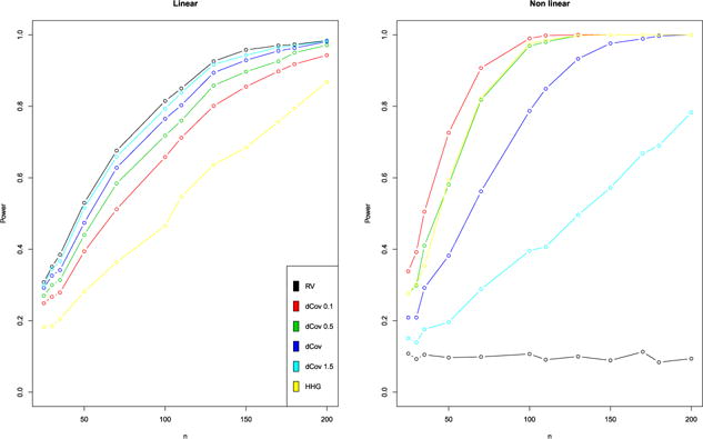
Power of the RV, dCov and HHG tests. Left: linear case. Right: non-linear case. The dCov test is performed using different exponents α (0.1, 1, 1.5, 2) on the Euclidean distances.

4.5. The Mantel coefficient

The Mantel [65, 61] coefficient, one of the earliest version of association measures, is probably also the most popular now, especially in ecology [102]. Given arbitrary dissimilarity matrices, it is defined as:

$${\mathrm{r}}_{\mathrm{m}}(\mathbf{X},\mathbf{Y})=\frac{{\displaystyle {\sum }_{i=1}^n{\displaystyle {\sum }_{j=1,j\ne 1}^n(d_{ij}^{\mathbf{X}}-{\overline{d}}^{\mathbf{X}})(d_{ij}^{\mathbf{Y}}-{\overline{d}}^{\mathbf{Y}})}}}{\sqrt{{\displaystyle {\sum }_{i,j,j\ne i}{(d_{ij}^{\mathbf{X}}-{\overline{d}}^{\mathbf{X}})}^2{\displaystyle {\sum }_{i,j,j\ne i}{(d_{ij}^{\mathbf{Y}}-{\overline{d}}^{\mathbf{Y}})}^2}}}},$$

with ${\stackrel{-}{d}}^{\mathbf{X}}$ (resp ${\stackrel{-}{d}}^{\mathbf{Y}}$) the mean of the upper diagonal terms of the dissimilarity matrix associated to X (resp. to Y). This is the correlation coefficient between the vectors gathering the upper diagonal terms of the dissimilarity matrices. The main difference between the Mantel coefficient and the others such as the RV or the dCov is the absence of double centering. Its significance is assessed via a permutation test. The coefficient and its test are implemented in several R packages such as ade4 [22], vegan [73] and ecodist [34].

Due to its popularity, many studies suggesting new coefficients often compared their performance to Mantel’s. Minas et al. [69] show that the Mantel test is less powerful than the test based on the GRV coefficient (4.1) using simulations. In the same way, Omelka and Hudecová [75] underlined the superiority of the dCov test over the Mantel test. However, despite its widespread use, some of the properties of the Mantel test are unclear and recently its utility questioned [75]. Legendre and Fortin [61] show that the Mantel coefficient is not equal to 0 when the covariance between the two sets of variables is null and thus can’t be used to detect linear relationships. Non-linear relationships can be detected, there are not yet clear theoretical results available to determine when.

Nevertheless, the extensive use in ecology and spatial statistics has led to a large number of extensions of the Mantel coefficient. Smouse et al. [101] proposed a generalization that can account for a third type of variable, i.e. allowing for partial correlations. Recently, the lack of power and high type I error rate for this test has been noted, calling into doubt the validity of its use [41]. Székely and Rizzo [107] also considered this extension to a partial correlation coefficient based on dCov.

5. Simulations

To compare performances of the dCov coefficient, the RV coefficient and the HHG test, we have run simulations similar in scope to those in [106].

First, matrices X_n×5 and Y_n×5 were generated from a multivariate Gaussian distribution with a within-matrix covariance structure equal to the identity matrix and the covariances between all the variables of X and Y equals to 0.1. We generated 1000 draws and computed the RV test (using the Pearson approximation) as well as the dCov test (using 500 permutations) for each draw. Figure 1, on the left, shows the power of the tests for different sample sizes n demonstrating the similar behavior of the RV (black curve) and dCov (dark blue curve) tests with a small advantage for the RV test. We also added the tests using different exponents α = (0.1, 0.5, 1.5) on the Euclidean distances which lead to different performances in terms of power. In addition, we included the results of the recent HHG test described in Section 4.4.

Then, another data structure was simulated by generating the matrix Y such that ${\mathbf{Y}}_{ml}=\mathit{log}({\mathbf{X}}_{ml}^2)$ for m, l = 1, …, 5 and the same procedure was applied. Results are displayed in Figure 1 on the right. As expected, the dCov tests are more powerful than the RV test in this non-linear setting.

These results show that the dCov detects linear relationships and has the advantage of detecting other associations, so is a considerable improvement on the RV and other ‘linear’ coefficients. However, it may still be worth using the RV coefficient for two reasons. First, with a significant dCov, it is impossible to know the pattern of association: are there only linear relationships between variables? only non-linear relationships or both kinds? Consequently, from a practical point of view, performing both the dCov and RV tests gives more insight into the nature of the relationship. When both coefficients are significant, we expect linear relationships between the variables of both groups. However, it does not mean that there are only linear relationships and non-linear relationships between the variables may occur as well. When only the dCov coefficient is significant then we expect only non-linear relationships but no information is available about the nature of these relationships. One should also take into account that the RV and related coefficients have had 30 years of use and the development of a large array of methods for dealing with multiway tables and heterogeneous multi-table data [54, 2, 27, 55, 22, 59, 77] that now allow the user to explore and visualize their complex multi-table data after assessing the significance of the associations. Consequently, these coefficients have become part of a broader strategy for analyzing heterogeneous data. We illustrate in Section 6 the importance of supplementing the coefficients and their test by graphical representations to investigate the significant relationships between blocks of variables.

Note that in the previous simulations, it is possible to test the significance of the relationship using classical likelihood ratio tests. For multivariate Gaussian data the parametric tests can be used [4] otherwise nonparametric tests based on ranks such as the one introduced in Puri and Sen [81] are available. Szekely et al. [106] compared the dCov test to some of the optimal ones showing similar power in the Gaussian case but better properties for non monotone relationships as expected. Cléroux et al. [15] show the similar power properties of the tests based on the RV.

6. Real data analysis

Since the dCov coefficient and the HHG test have higher power than other coefficients (RV or the Procrustes) to measure departure from independence, it would be worthwhile for the ecologists, food-scientists and other scientists in applied fields to try the dCov and HHG methods on their data. In this section, we illustrate the use of the coefficients and tests on real data from different fields. We used the dCov, the RV, the Procrustes and the Lg coefficients and the HHG test as well as an implementation of the graph based method of Friedman and Rafsky [30]. We emphasize the complementarity of the different coefficients as well as the advantage of providing follow-up graphical representations. Many multi-block methods that use the earlier RV can be adapted to incorporate the other approaches. We have implemented this in our examples for which the code, allowing full reproducibility, is available as supplementary material.

6.1. Sensory analysis

6.1.1. Reproducibility of tasting experiments

Eight wines from Jura (France) were evaluated by twelve panelists. Each panelist tasted the wines and positioned them on a 60×40 cm sheet of paper such that two wines are close if they seem similar to the taster, and farther apart if they seem different. Then, the coordinates are collected in a 8 × 2 matrix. This way of collecting sensory data is named “napping” [76] and encourages spontaneous description. The 8 wines were evaluated during 2 sessions (with an interval of a few days). There are as many matrices as there are couple taster-sessions (24 = 12 × 2). As with any data collection procedure, the issue of repeatability arises here. Are the product configurations given by a taster roughly the same from one session to the other? In other words, do they perceive the wines in a same way during the two sessions? This question was addressed in Josse et al. [48] by using the RV between the configurations obtained during sessions 1 and 2 for all the panelists, we also show the HHG test and dCov coefficient with different exponents on the distances. Results have been combined in Table 1.

Table 1.

Coefficients of association and tests between the configuration of the 12 tasters obtained during session 1 and session 2: RV coefficient and its p-value RV_p, dCor coefficient and its p-value, p-values associated with the dCov test with exponents α on the distance equal to 0.1, 0.5 and 1.5 as well as the HHG test. The RV test used Pearson’s approximation; the other tests were done with 1000 permutations.

	RV	RVp	dCor	dCovp	dCovp0.1	dCovp0.5	dCovp1.5	HHGp
1	0.55	0.04	0.10	0.09	0.16	0.13	0.13	0.07
2	0.22	0.60	0.72	0.76	0.84	0.81	0.81	0.30
3	0.36	0.16	0.68	0.32	0.55	0.43	0.44	0.62
4	0.13	0.68	0.84	0.76	0.51	0.65	0.65	0.90
5	0.64	0.02	0.01	0.02	0.04	0.03	0.03	0.04
6	0.14	0.56	0.54	0.75	0.83	0.81	0.81	0.73
7	0.79	0.01	0.91	0.01	0.01	0.01	0.01	0.02
8	0.06	0.82	0.81	0.76	0.65	0.70	0.70	0.89
9	0.49	0.04	0.28	0.11	0.28	0.25	0.25	0.29
10	0.28	0.29	0.29	0.24	0.17	0.20	0.20	0.24
11	0.22	0.40	0.39	0.26	0.19	0.23	0.22	0.36
12	0.19	0.54	0.58	0.55	0.58	0.57	0.56	0.09

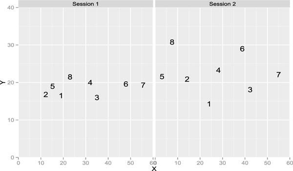
The methods show that tasters 5 and 7 are repeatable. For tasters 1 and 9, only the RV coefficient rejects the null, the p-value of the HHG test is borderline at 0.07. Note that we performed the other versions of the HHG test (for instance with the statistic defined with the max of the Chi-square instead of the sum [49]) and they only give taster 7 as repeatable. Figures 2 and 3 give the representation during the first and second sessions. Taster 9 distinguished 3 clusters of wines but switched the wines 6 and 7 from one session to the other. It is more difficult to understand why the RV coefficient is significant when inspecting the configurations given by taster 1, as the RV is invariant by rotation, we rotated the second configuration onto the first one on Figure 4. The pattern looks more similar with wines 6 and 7 quite close and the wine 4 far from the others. Figure 5 gives the representation provided by taster 7 to show a case with a consensus between the tests. On this real data set, it is impossible to know the ground truth but the RV test shows that two panelists can be considered as reliable.

Fig 2.

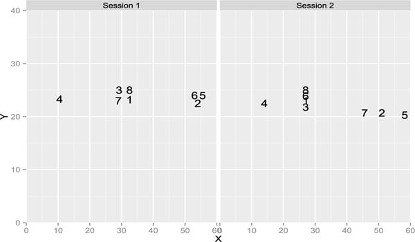
Representation of the 8 wines on the 40 × 60 sheet of paper given by the panelist 9 during session 1 and 2.

Fig 3.

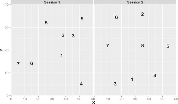
Representation of the 8 wines on the 40 × 60 sheet of paper given by the panelist 1 during session 1 and 2.

Fig 4.

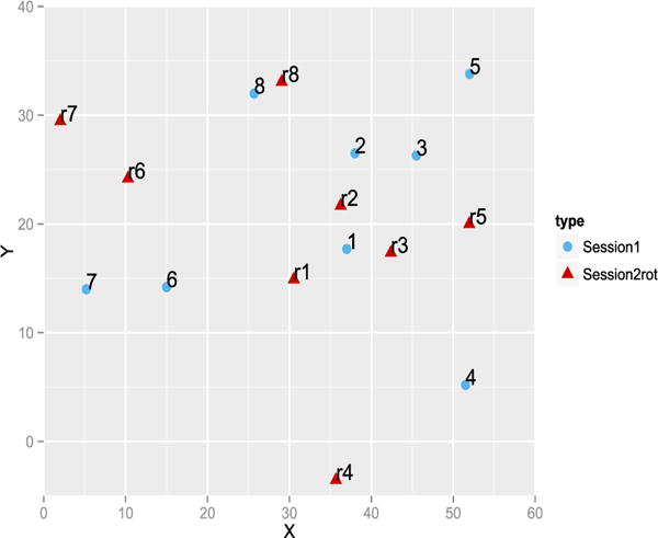
Representation of the rotated configuration of the session 2 (red triangles) onto the session 1’s configuration for panelist 1.

Fig 5.

Representation of the 8 wines on the 40 × 60 sheet of paper given by the panelist 7 during session 1 and 2.

6.1.2. Panel comparison

Six French chocolates were evaluated by 7 panels with a total of 29 judges who grade 14 sensory descriptors such as bitterness, crunchy, taste of caramel, etc. For each panel, the data matrix is of size 6 × 14 and each cell corresponds to the average of the scores given for one chocolate on a descriptor by the judges (ranging from 1 for not bitter to 10 for very bitter for instance). One aim of the study was to see if the panels produce concordant descriptions of the products. Tables 2 and 3 show the matrices of RV and dCor coefficients. All the coefficients are very high and are highly significant.

Table 2.

RV coefficients between the matrices products-descriptors provided by the 7 panels.

	1	2	3	4	5	6	7
1	1.000	0.989	0.990	0.984	0.985	0.995	0.993
2		1.000	0.992	0.991	0.993	0.996	0.997
3			1.000	0.995	0.992	0.996	0.997
4				1.000	0.983	0.993	0.993
5					1.000	0.994	0.997
6						1.000	0.999
7							1.000

Table 3.

dCor coefficients between the matrices products-descriptors provided by the 7 panels.

	1	2	3	4	5	6	7
1	1.000	0.986	0.983	0.974	0.977	0.991	0.991
2		1.000	0.984	0.981	0.978	0.996	0.995
3			1.000	0.984	0.987	0.993	0.994
4				1.000	0.956	0.988	0.986
5					1.000	0.983	0.989
6						1.000	0.999
7							1.000

After seeing a significant association, we analyze the RV matrix by a multi-block method such as STATIS [27]. The rationale of STATIS is to consider the matrix of RV’s as a matrix of inner products. Consequently, an Euclidean representation of the inner products reduced to a lower-dimensional space by performing the eigenvalue decomposition of the matrix. This first step of STATIS, named the “between-structure” analysis, produces a graphical representation of the proximity between tables in a consensus space. This can be quite useful when there are many blocks of variables. This is equivalent to performing multidimensional scaling (MDS or PCoA) [35] on the associated distance matrix. The same reasoning is valid for a matrix of dCor coefficients and thus we also show this approach on the dCor matrix. Figure 6 is the result of such an analysis and shows that there is strong consensus between the description of the chocolates provided by the 7 panels since the 7 panels are very close.

Fig 6.

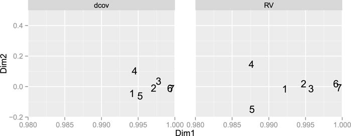
Graphical representation of the proximity between panels with the proximity defined with the dCor coefficient (on the left) and with the RV coefficient (on the right).

The STATIS method goes deeper by showing what is common between the 7 panels (called the “compromise” step) and then what is specific to each panel in the “within-structure” step. The use of such a two step approach can also be undertaken using the dCov coefficients. The “compromise” representation is obtained by looking for a similarity matrix $\overline{\mathbf{W}}$ which is the more related to all the inner product matrices (here K=7) in the following sense: $\overline{\mathbf{W}}={\text{argmax}}_{\mathbf{W}\ast ={\displaystyle {\sum }_{k=1}^K\gamma k}{\mathbf{W}}_k;{\displaystyle {\sum }_k{\gamma }_k^2=1}}{{\displaystyle {\sum }_{k=1}^K<\mathbf{W}\ast ,{\mathbf{W}}_k>}}^2$. The weights γ_k are given by the first eigenvector of the RV matrix and are positive since all the elements of the RV matrix are positive (using the Frobenius theorem). Then an Euclidean representation of the compromise object $\overline{\mathbf{W}}$ is also obtained by performing the eigen decomposition and is given Figure 7. It shows that all the 7 panels distinguished chocolate 3 from the others. We do not detail the sequel of the analysis which would consist in looking at why the chocolate 3 is so different from the other, etc.

Fig 7.

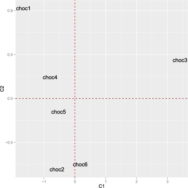
Representation of the STATIS compromise.

Note that one could also consider the analogous of STATIS for kernels and use the compromise kernel: a linear combination of kernels with optimal weights.

6.2. Microarray data

We continue the example discussed in the introduction on the 43 brain tumors described with expression data (356 variables) and CGH data (76 variables).

6.2.1. Distance based coefficients

To compare the two different types of information we first compute association coefficients. A high value of a coefficient would indicate that when tumors have similar transcriptomes, they are also similar from the genomic viewpoint. The RV coefficient is equal to 0.34. Section 2.3 show the importance of computing a biased-corrected version of the coefficient especially when dealing with large data. We have corrected the RV by removing its expectation under the null defined equation (2.6) which is equal to ${\mathbb{E}}_{H_0}(\text{RV})$. The dCor coefficient is equal to 0.74 and its biased-corrected version dCor* to 0.28. These coefficients are significant, as is HHG test with a p-value of 0.04.

6.2.2. Graph based coefficients

Here we implemented the coefficients defined in Friedman and Rafsky [30] (described Section 4.3) using both the minimum spanning trees and the k nearest-neighbor trees. The former show very little association and seems to have very little power in high dimensions, the two minimum spanning trees only had three edges in common out of 42. However, as shown in Figure 8, the k nearest-neighbor version (with k=5) is significant with a p-value smaller than 0.004.

Fig 8.

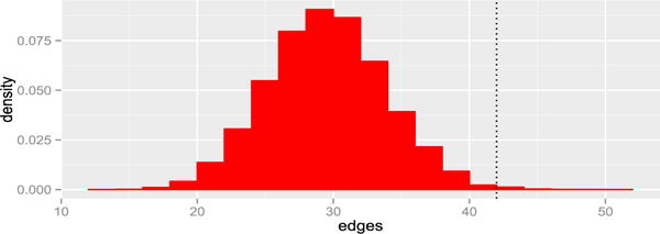
Histogram of the permutation distribution of Friedman and Rafsky’s k nearest-neighbor graphs’ common edges with k=5, the observed value was 42 for the original data.

6.2.3. Graphical exploration of associations

The previous results and simulations point to the existence of some linear relationships between the variables in the two domains. To study and visualize the associations, different multi-block methods such as STATIS are available [54]. Here we take a different approach using multiple factor analysis (MFA) described in [77]. This method uses the L_g coefficient described in Section 2.5.3. The L_g coefficient for the expression data is equal to 1.09 whereas it is 2.50 for the CGH data which means that the expression data may be have a univariate latent structure whereas the CGH data is more multi-dimensional. MFA gives as an output Figure 9 on the left which is the equivalent of the “between-structure” step of Section 6.1.2. Here, the coordinates of the domains correspond to the values of the L_g coefficient between the dimensions of the “compromise” and each block. Thus we see that first dimension is common to both blocks of variables whereas the second dimension is mainly due to the group CGH. We are also able to say that this first dimension is close to the first principal component of each block since the values of the L_g are close to one (as explained in Section 2.5.3). Figure 9 on the right is the equivalent of the “compromise” step of Section 6.1.2 and shows that the first dimension of variability opposes the glioblastomas tumors to the lower grade tumors and that the second dimension opposes tumors O to the tumors OA and A. The first dimension is common to both blocks of variables, this means that both the expression data and the CGH data separates the glioblastomas from the other tumors. On the other hand, only the CGH data contrasts the O tumor with the tumors OA and A. This shows what is common and what is specific to each block. Figure 10 on the left is the correlation circle showing the correlations between all the variables and we see that the expression data is one-dimensional whereas the CGH data is at least on two dimensional (red arrows are hidden by the green arrows) as expected given the L_g coefficient values. This method also allows comparisons at the observation level with a “partial” representation represented Figure 10 on the right. The tumor GBM29 is represented using only its expression data (in green) and using only its CGH data (in red). The black dot is at the barycenter of both red and green points and represents the tumor GBM29 using all the data. This tumor is peculiar in the sense that when taking its CGH data, it is on the side of the dangerous tumors (small coordinates on the first axis) whereas it is on the side of the other tumors when one only considers its expression data (positive coordinates on the first axis). There is no consensus between the two sources of information for this particular sample and additional data is necessary to understand why. More details about this particular method and aids to its interpretation can be found in [77]. Note that only linear relationships have been explored here and that potential non-linear relationships highlighted by the dCov or the HHG test were not plotted.

Fig 9.

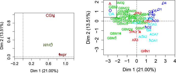
MFA groups representation (left) and compromise representation of the tumors (right).

Fig 10.

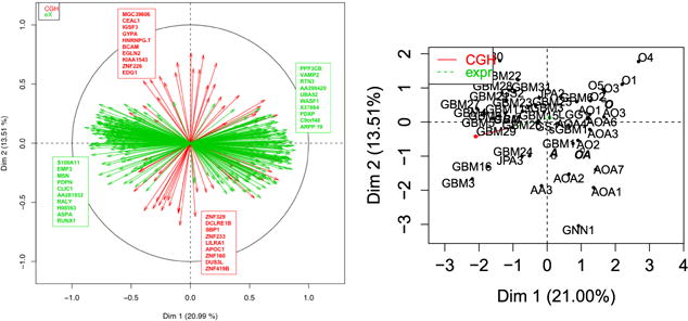
MFA variables representation (left) and a “partial” sample (right).

6.3. Morphology data set

In cephalofacial growth studies, shape changes are analysed by recording landmark positions at different ages. We focus here on a study on male macaca nemestrina skull described in Olshan et al. [74]. Figure 11 gives 72 landmarks of a macaca at the age of 0.9 and 5.77 years. To study the similarity between the two configurations, we compute the association coefficients and tests. The RV coefficient is 0.969 (its unbiased version is 0.94) and the dCor coefficient is 0.99 (its unbiased version is 0.985) and they are highly significant. The HHG test is also highly significant. The standard coefficient used on morphological landmark data is the Procrustes coefficient described Section 2.5.2. Procrustes analysis superimposes different configurations as illustrated Figure 12 on the left. The dots represent the shape at age 0.9 years and the arrows point to the shape at 5.77 years obtained after translation and rotation. Figure 12 on the right represents the permutation distribution of the Procrustes coefficient under the null and the straight line indicates its observed value which is 0.984. The p-value associated to the test is thus very small.

Fig 11.

Macaca landmarks at 0.9 and 5.77 years.

Fig 12.

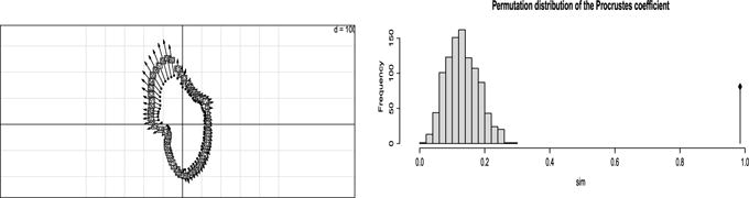
Left: Procrustes analysis to represent the deformation from 0.9 to 5.77 years of the macaca face. Right: Permutation distribution of the Procrustes coefficient and its observed value.

6.4. Chemometry data set

In the framework of the EU TRACE project², spectroscopic techniques are used to identify and guarantee the authenticity of products such as the Trappist Rochefort 8 degree beer (one of seven authentic Trappist beers in the world). The data which were presented as a challenge at the annual French Chemometry meeting in 2010³ consist of 100 beers measured using three vibrational spectroscopic techniques: near infrared (NIR), mid-infrared (MIR) and Raman spectroscopy. The beers were analysed twice using the same instruments, providing technical replicates. Table 4 shows the similarity between the repetitions. Raman’s spectral repetitions are stable whereas the other two methods are not. Table 5 studies the similarities between measurments and shows that it provides complementary information since the values of the coefficients are quite small.

Table 4.

Similarity between two measurements on the same 100 beers with different spectroscopic methods (NIR, MIR, Raman). RV coefficient and its bias-corrected version RV* and the dCor coefficient and its bias-corrected version dCor*.

	RV	RV *	dCor	dCor*
NIR	0.298	0.297	0.709	0.482
MIR	0.597	0.595	0.798	0.585
Raman	0.978	0.977	0.987	0.974

Table 5.

Similarity between the spectroscopic techniques (NIR, MIR, Raman). Bias-corrected RV coefficient RV* and dCor coefficient dCor*.

	RV* coefficient			dCor* coefficient
	NIR	MIR	Raman	NIR	MIR	Raman
NIR	1	0.03	0.33	1	0.07	0.45
MIR		1	0.03		1	0.05
Raman			1			1

7. Conclusion

Technological advances are leading to the collection of many different types of data on the same samples (images, metabolic characteristics, genetic profiles or clinical measurements). These heterogeneous sources of information can lead to improved explanatory resolution and power in the statistical analyses. We have discussed several coefficients of association presented as functions of general dissimilarity (or similarity) matrices that are convenient for comparing heterogeneous data. We have outlined how to go beyond the calculation of these coefficients and make sense of the associations between these disparate sources of information. We can localize the dependence and distinguish which variables are more involved in the relationship between tables.

The HHG test is consistent against all dependent alternatives when there exists a point where the joint distribution is continuous (see Heller et al. [43]) whereas dCov requires finite first moment conditions to be consistent. On the other hand, classical tests such as the CC or RV coefficients are consistent but designed to detect simple linear relationships (although the use of relevant variable transformations can overcome this flaw). In practice, we recommend computation of both linear and nonlinear measures such as the RV and the dCov coefficients and their bias-corrected version to gain more insight into the nature of the relationships. In addition, we suggest to supplement an association study, a follow-up analysis with graphical output allows the scientist to explore and visualize the complex multi-table data. We have described STATIS and MFA which rely on linear relationships between variables; the success with which these methods have allowed psychometricians, ecologists and food scientists to describe their data suggests that adapting them to incorporate nonlinear coefficients such as dCov could be a worthwhile enterprise.

In this survey, our focus has been on continuous variables and some comments can be made on the case of categorical variables or a hybrid collection of continuous and categorical ones. Users of multiple correspondence analyses [39] have developed special weighting metrics for contingency tables and indicator matrices of dummy variables that replace correlations and variances with chi-square based statistics. With specific row and column weights, it has been shown that the RV coefficient between two groups of categorical variables is related to the sum of the Φ² between all the variables and the RV between one group of continuous and one group of categorical variables to the sum of the squared correlation ratio η² between the variables [28, 44, 77]. Another approach suggested by Friedman and Rafsky [30] was to use Hamming distance to build graphs from categorical variables.

Many of the discussed coefficients use the sample covariance matrices to estimate the population covariance matrices. The current evolution of estimation of such quantities reveals that better results in term of mean squared error can be obtained by considering regularized versions of such matrices while shrinking and thresholding the singular values [8, 60, 13]. This is certainly a topic requiring further study.

Finally, all results depend on the particular preprocessing choice (such as scaling), distance or kernel choices. This flexibility can be viewed as a strength, since many types of dependencies can be discovered. On the other hand, of course, it underscores the subjectivity of the analysis and the importance of educated decisions made by the analyst and downstream sensitivity analyses.

References

- 1.Abdi H. Congruence: Congruence coefficient, RV coefficient, and Mantel coefficient. In: Salkind NJ, Dougherty DM, Frey B, editors. Encyclopedia of Research Design, pages. Thousand Oaks (CA): Sage; 2010. pp. 222–229. [Google Scholar]
- 2.Acar E, Yener B. Unsupervised multiway data analysis: A literature survey. Knowledge and Data Engineering, IEEE Transactions on. 2009;21(1):6–20. [Google Scholar]
- 3.Allaire J, Lepage Y. On a likelihood ratio test for independence. Statistics & Probability Letters. 1991;11(5):449–452. [Google Scholar]
- 4.Anderson TW. An Introduction to Multivariate Statistical Analysis. 3rd. Wiley; 2003. [Google Scholar]
- 5.Barton DE, David FN. Randomization bases for multivariate tests. I. The bivariate case. Randomness of n points in a plane. Bulletin of the international statistical institute. 1962:i39. [Google Scholar]
- 6.Beran R, Bilodeau M, Lafaye de Micheaux P. Nonparametric tests of independence between random vectors. Journal of Multivariate Analysis. 2007;98(9):1805–1824. [Google Scholar]
- 7.Bergsma W, Dassios A. A consistent test of independence based on a sign covariance related to kendall’s tau. Bernoulli. 2014;20(2):1006–1028. [Google Scholar]
- 8.Bickel PJ, Levina E. Regularized estimation of large covariance matrices. The Annals of Statistics. 2008;36(1):199–227. [Google Scholar]
- 9.Bilodeau M, Lafaye de Micheaux P. A multivariate empirical characteristic function test of independence with normal marginals. Journal of Multivariate Analysis. 2005;95:345–369. [Google Scholar]
- 10.Borg I, Groenen PJF. Modern Multidimensional Scaling: Theory and Applications. Springer; 2005. [Google Scholar]
- 11.Cadena RS, Cruz AG, Netto RR, Castro WF, Faria J-D-AF, Bolini HMA. Sensory profile and physicochemical characteristics of mango nectar sweetened with high intensity sweeteners throughout storage time. Food Research International. 2013 [Google Scholar]
- 12.Cailliez F. The analytical solution of the additive constant problem. Psychometrika. 1983;48(2):305–308. [Google Scholar]
- 13.Chatterjee S. Matrix estimation by universal singular value thresholding. The Annals of Statistics. 2014;43(1):177–214. [Google Scholar]
- 14.Cléroux R, Ducharme GR. Vector correlation for elliptical distribution. Communications in Statistics Theory and Methods. 1989;18:1441–1454. [Google Scholar]
- 15.CLéroux R, Lazraq A, Lepage Y. Vector correlation based on ranks and a non parametric test of no association between vectors. Communications in Statistics Theory and Methods. 1995;24:713–733. [Google Scholar]
- 16.Cramer EM, Nicewander WA. Some symmetric, invariant measures of mutivariate association. Psychometrika. 1979;44(1):43–54. [Google Scholar]
- 17.Cristianini N, Shawe-Taylor J, Elisseeff A, Kandola J. On kernel-target alignment. NIPS. 2001 [Google Scholar]
- 18.Culhane A, Perrière G, Higgins D. Cross-platform comparison and visualisation of gene expression data using co-inertia analysis. BMC bioinformatics. 2003;4(1):59. doi: 10.1186/1471-2105-4-59. [DOI] [PMC free article] [PubMed] [Google Scholar]
- 19.David FN, Barton DE. Combinatorial chance. Griffin; London: 1962. [Google Scholar]
- 20.David FN, Barton DE. Two space-time interaction tests for epidemicity. British Journal of Preventive & Social Medicine. 1966;20(1):44–48. [Google Scholar]
- 21.de Tayrac M, Le S, Aubry M, Mosser J, Husson F. Simultaneous analysis of distinct omics data sets with integration of biological knowledge: Multiple factor analysis approach. BMC Genomics. 2009;10(1):32–52. doi: 10.1186/1471-2164-10-32. [DOI] [PMC free article] [PubMed] [Google Scholar]
- 22.Dray S. The ade4 package: implementing the duality diagram for ecologists. Journal of Statistical Software. 2007;22(4):1–20. [Google Scholar]
- 23.Dray S, Chessel D, Thioulouse J. Procrustean co-inertia analysis for the linking of multivariate datasets. Ecoscience. 2003;10:110–119. [Google Scholar]
- 24.Escofier B, Pagès J. Multiple factor analysis (afmult package) Computational Statistics & Data Analysis. 1994;18(1):121–140. [Google Scholar]
- 25.Escoufier Y. Echantillonnage dans une population de variables aléatoires réelles. Department de math.; Univ des sciences et techniques du Languedoc; 1970. [Google Scholar]
- 26.Escoufier Y. Le traitement des variables vectorielles. Biometrics. 1973;29:751–760. [Google Scholar]
- 27.Escoufier Y. Method for multidimensional analysis. Lecture notes from the European Course in Statistic; 1987. Three-mode data analysis: the STATIS method; pp. 153–170. [Google Scholar]
- 28.Escoufier Y. Compstat 2006-Proceedings in Computational Statistics. Springer; 2006. Operator related to a data matrix: a survey; pp. 285–297. [Google Scholar]
- 29.Foth C, Bona P, Desojo JB. Intraspecific variation in the skull morphology of the black caiman melanosuchus niger (alligatoridae, caimaninae) Acta Zoologica. 2013 [Google Scholar]
- 30.Friedman JH, Rafsky LC. Graph-theoretic measures of multivariate association and prediction. Annals of Statistics. 1983;11(2):377–391. [Google Scholar]
- 31.Fruciano C, Franchini P, Meyer A. Resampling-based approaches to study variation in morphological modularity. PLoS ONE. 2013;8:e69376. doi: 10.1371/journal.pone.0069376. [DOI] [PMC free article] [PubMed] [Google Scholar]
- 32.Génard M, Souty M, Holmes S, Reich M, Breuils L. Correlations among quality parameters of peach fruit. Journal of the Science of Food and Agriculture. 1994;66(2):241–245. [Google Scholar]
- 33.Giacalone D, Ribeiro LM, Frøst MB. Consumer-based product profiling: Application of partial napping® for sensory characterization of specialty beers by novices and experts. Journal of Food Products Marketing. 2013;19(3):201–218. [Google Scholar]
- 34.Goslee SC, Urban DL. The ecodist package for dissimilarity-based analysis of ecological data. Journal of Statistical Software. 2007;22:1–19. [Google Scholar]
- 35.Gower JC. Some distance properties of latent root and vector methods used in multivariate analysis. Biometrika. 1966;53:325–338. [Google Scholar]
- 36.Gower JC. Statistical methods of comparing different multivariate analyses of the same data. In: Hodson FR, Kendall DG, Tautu P, editors. Mathematics in the archaeological and historical sciences. Edinburgh University Press; 1971. pp. 138–149. [Google Scholar]
- 37.Greenacre MJ. Correspondence analysis of multivariate categorical data by weighted least-squares. Biometrika. 1988;75:457–477. [Google Scholar]
- 38.Greenacre MJ. Multiple and joint correspondence analysis. In: Blasius J, Greenacre MJ, editors. Correspondence Analysis in the social science. London: Academic Press; 1994. pp. 141–161. [Google Scholar]
- 39.Greenacre MJ, Blasius J. Multiple Correspondence Analysis and Related Methods. Chapman & Hall/CRC; 2006. [Google Scholar]
- 40.Gretton A, Herbrich R, Smola A, Bousquet O, Schoelkopf B. Kernel methods for measuring independence. Journal of Machine Learning Research. 2005;6:2075–2129. [Google Scholar]
- 41.Guillot G, Rousset F. Dismantling the Mantel tests. Methods in Ecology and Evolution. 2013 [Google Scholar]
- 42.Heller R, Gorfine M, Heller Y. A class of multivariate distribution-free tests of independence based on graphs. Journal of Statistical Planning and Inference. 2012;142(12):3097–3106. doi: 10.1016/j.jspi.2012.06.003. [DOI] [PMC free article] [PubMed] [Google Scholar]
- 43.Heller R, Heller Y, Gorfine M. A consistent multivariate test of association based on ranks of distances. Biometrika. 2013;100(2):503–510. [Google Scholar]
- 44.Holmes S. Probability and Statistics: Essays in Honor of David A Freedman. Institute of Mathematical Statistics; Beachwood, Ohio: 2008. Multivariate data analysis: the French way; pp. 219–233. [Google Scholar]
- 45.Hotelling H. Relations between two sets of variants. Biometrika. 1936;28:321–377. [Google Scholar]
- 46.Husson F, Josse J, Le S, Mazet J. FactoMineR: Multivariate Exploratory Data Analysis and Data Mining with R. 2013 URL http://CRAN.R-project.org/package=FactoMineR R package version 1.24.
- 47.Jackson DA. Protest: a procustean randomization test of community environment concordance. Ecosciences. 1995;2:297–303. [Google Scholar]
- 48.Josse J, Pagès J, Husson F. Testing the significance of the RV coefficient. Computational Statistics and Data Analysis. 2008;53:82–91. [Google Scholar]
- 49.Kaufman S. HHG: Heller-Heller-Gorfine Tests of Independence. 2014 URL http://CRAN.R-project.org/package=HHG R package version 1.4.
- 50.Kazi-Aoual F, Hitier S, Sabatier R, Lebreton JD. Refined approximations to permutation tests for multivariate inference. Computational Statistics and Data Analysis. 1995;20:643–656. [Google Scholar]
- 51.Klingenberg CP. Morphometric integration and modularity in configurations of landmarks: tools for evaluating a priori hypotheses. Evolution & Development. 2009;11:405–421. doi: 10.1111/j.1525-142X.2009.00347.x. [DOI] [PMC free article] [PubMed] [Google Scholar]
- 52.Knox EG. The detection of space-time interactions. Journal of the Royal Statistical Society Series C (Applied Statistics) 1964;13(1):25–30. [Google Scholar]
- 53.Kojadinovic I, Holmes M. Tests of independence among continuous random vectors based on cramér-von mises functionals of the empirical copula process. Journal of Multivariate Analysis. 2009;100(6):1137–1154. [Google Scholar]
- 54.Kroonenberg PM. Applied Multiway Data Analysis Wiley series in probability and statistics. 2008 [Google Scholar]
- 55.Lavit C, Escoufier Y, Sabatier R, Traissac P. The ACT (STATIS method) Computational Statistics & Data Analysis. 1994;18(1):97–119. [Google Scholar]
- 56.Lazraq A, Cleroux R. Statistical inference concerning several redundancy indices. Journal of Multivariate Analysis. 2001;79(1):71–88. [Google Scholar]
- 57.Lazraq A, Robert C. Etude comparative de diffèrentes mesures de liaison entre deux vecteurs aléatoires et tests d’indépendance. Statistique et analyse de données. 1988;1:15–38. [Google Scholar]
- 58.Lazraq A, Cléroux R, Kiers HAL. Mesures de liaison vectorielle et généralisation de l’analyse canonique. Statistique et analyse de données. 1992;40(1):23–35. [Google Scholar]
- 59.Lê S, Josse J, Husson F. Factominer: An r package for multi-variate analysis. Journal of Statistical Software. 2008;25(1):1–18. 3. [Google Scholar]
- 60.Ledoit O, Wolf M. Nonlinear shrinkage estimation of large-dimensional covariance matrices. The Annals of Statistics. 2012;40(2):1024–1060. [Google Scholar]
- 61.Legendre P, Fortin M. Comparison of the Mantel test and alternative approaches for detecting complex multivariate relationships in the spatial analysis of genetic data. Molecular Ecology Resources. 2010;10:831–844. doi: 10.1111/j.1755-0998.2010.02866.x. [DOI] [PubMed] [Google Scholar]
- 62.Lingoes JC, Schönemann PH. Comparison of the Mantel test and alternative approaches for detecting complex multivariate relationships in the spatial analysis of genetic data. Psychometrika. 1974;39:423–427. doi: 10.1111/j.1755-0998.2010.02866.x. [DOI] [PubMed] [Google Scholar]
- 63.Lingoes JC. Some boundary conditions for a monotone analysis of symmetric matrices. Psychometrika. 1971;36(2):195–203. [Google Scholar]
- 64.Lopez-Paz D, Hennig P, Schölkopf B. The Randomized Dependence Coefficient. NIPS. 2013 [Google Scholar]
- 65.Mantel N. The detection of disease clustering and a generalized regression approach. Cancer research. 1967;27(2 Part 1):209–220. [PubMed] [Google Scholar]
- 66.Mardia KV, Kent JT, Bibby JM. Multivariate analysis Academic press. 1980 [Google Scholar]
- 67.MATLAB. MATLAB and Statistics Toolbox Release. The Math-Works, Inc; Natick, Massachusetts, United States: 2012. URL http://www.mathworks.com/products/matlab/ [Google Scholar]
- 68.Mayer CD, Lorent T, Horgan GW. Exploratory analysis of multiples omics datasets using the adjusted RV coefficient. Statistical applications in genetics and molecular biology. 2011;10 doi: 10.2202/1544-6115.1540. [DOI] [PubMed] [Google Scholar]
- 69.Minas C, Curry E, Montana G. A distance-based test of association between paired heterogeneous genomic data. Bioinformatics. 2013;29(22):2555–2563. doi: 10.1093/bioinformatics/btt450. [DOI] [PubMed] [Google Scholar]
- 70.Nelsen RB. An Introduction to Copulas. 2nd. Springer Science+Buisness; New York: 2006. [Google Scholar]
- 71.Newton MA. Introducing the discussion paper by szekely and rizzo. The Annals of Applied Statistics. 2009;3(4):1233–1235. [Google Scholar]
- 72.Noble AC, Ebeler SE. Use of multivariate statistics in understanding wine flavor. Food Reviews International. 2002;18(1):1–20. [Google Scholar]
- 73.Oksanen J, Blanchet FG, Kindt R, Legendre P, Minchin PR, O’Hara RB, Simpson GL, Solymos P, Stevens MH, Wagner H. vegan: Community Ecology Package. 2013 URL http://CRAN.R-project.org/package=vegan. R package version 2.0-9.
- 74.Olshan AF, Siegel AF, Swindler DR. Robust and least-squares orthogonal mapping: Methods for the study of cephalofacial form and growth. American Journal of Physical Anthropology. 1982;59(2):131–137. doi: 10.1002/ajpa.1330590203. [DOI] [PubMed] [Google Scholar]
- 75.Omelka M, Hudecová S. A comparison of the mantel test with a generalised distance covariance test. Environmetrics. 2013 [Google Scholar]
- 76.Pagès J. Collection and analysis of perceived product inter-distances using multiple factor analysis; application to the study of ten white from the loire valley. Food quality and preference. 2005;16:642–649. [Google Scholar]
- 77.Pagès J. Multiple Factor Analysis with R. Chapman & Hall/CRC; 2014. [Google Scholar]
- 78.Pagès J, Husson F. Multiple factor analysis with confidence ellipses: A methodology to study the relationships between sensory and instrumental data. Journal of Chemometrics. 2005;19:138–144. [Google Scholar]
- 79.Peres-Neto PR, Jackson DA. How well do multivariate data sets match? the advantages of a procrustean superimposition approach over the mantel test. Oecologia. 2001;129:169–178. doi: 10.1007/s004420100720. [DOI] [PubMed] [Google Scholar]
- 80.Purdom E. PhD thesis. University of Stanford; 2006. Multivariate kernel methods in the analysis of graphical structures. [Google Scholar]
- 81.Puri ML, Sen PK. Nonparametric Methods in Multivariate Analysis. John Wiley & Sons; New York: 1974. [Google Scholar]
- 82.Quessy JF. Applications and asymptotic power of marginal-free tests of stochastic vectorial independence. Journal of Statistical Planning and Inference. 2010;140(11):3058–3075. [Google Scholar]
- 83.R core Team. R: A Language and Environment for Statistical Computing. R Foundation for Statistical Computing; Vienna, Austria: 2013. URL http://www.R-project.org/ [Google Scholar]
- 84.Ramsay JO, ten Berge J, Styan GPH. Matrix correlation. Psychometrika. 1984;49(3):403–423. [Google Scholar]
- 85.Reimherr M, Nicolae DL. On quantifying dependence: A framework for developing interpretable measures. Statistical Science. 2013;28(1):116–139. [Google Scholar]
- 86.Renyi A. On measures of dependence. Acta Mathematica Academiae Scientiarum Hungarica. 1959;10(3–4):441–451. [Google Scholar]
- 87.Risvik E, McEwan JA, Rødbotten M. Evaluation of sensory profiling and projective mapping data. Food quality and preference. 1997;8(1):63–71. [Google Scholar]
- 88.Rizzo ML, Szekely GJ. energy: E-statistics (energy statistics) 2013 URL http://CRAN.R-project.org/package=energy. R package version 1.6.0.
- 89.Robert P, Escoufier Y. A unifying tool for linear multivariate statistical methods: The RV- coefficient. Journal of the Royal Statistical Society Series C (Applied Statistics) 1976;3:257–265. [Google Scholar]
- 90.Robert P, Cléroux R, Ranger N. Some results on vector correlation. Computational Statistics and Data Analysis. 1985;3:25–32. [Google Scholar]
- 91.Rohlf FJ, Slice D. Extensions of the procrustes method for the optimal superimposition of landmarks. Systematic Biology. 1990;39(1):40–59. [Google Scholar]
- 92.Romano JP. A bootstrap revival of some nonparametric distance tests. Journal of the American Statistical Association. 1988;83(403):698–708. [Google Scholar]
- 93.Romano JP. Bootstrap and randomization tests of some nonparametric hypotheses. The Annals of Statistics. 1989;17(1):141–159. [Google Scholar]
- 94.Santana SE, Lofgren SE. Does nasal echolocation influence the modularity of the mammal skull? Journal of evolutionary biology. 2013;26(11):2520–2526. doi: 10.1111/jeb.12235. [DOI] [PubMed] [Google Scholar]
- 95.Schlich P. Defining and validating assessor compromises about product distances and attribute correlations. Data handling in science and technology. 1996;16:259–306. [Google Scholar]
- 96.Schoenberg IJ. Remarks to maurice fréchet’s article “sur la définition axiomatique d’une classe d’espace distancié vectoriellement applicable sur l’espace de hilbert. Annals of Mathematics. 1935;36(2):724–732. [Google Scholar]
- 97.Scholkopf B, Smola AJ. Learning with Kernels: Support Vector Machines, Regularization, Optimization, and Beyond. MIT Press; Cambridge, MA, USA: 2001. [Google Scholar]
- 98.Sejdinovic D, Sriperumbudur B, Gretton A, Fukumizu K. Equivalence of distance-based and rkhs-based statistics in hypothesis testing. Annals of Statistics. 2013;41:2263–2291. [Google Scholar]
- 99.Shinkareva SV, Mason RA, Malave VL, Wang W, Mitchell TM, Just MA. Using fmri brain activation to identify cognitive states associated with perception of tools and dwellings. PLoS One. 2008;3(1):e1394. doi: 10.1371/journal.pone.0001394. [DOI] [PMC free article] [PubMed] [Google Scholar]
- 100.Smilde AK, Kiers HAL, Bijlsma S, Rubingh CM, van Erk MJ. Matrix correlations for high-dimensional data: the modified RV-coefficient. Bioinformatics. 2009;25:401–405. doi: 10.1093/bioinformatics/btn634. [DOI] [PubMed] [Google Scholar]
- 101.Smouse PE, Long JC, Sokal RR. Multiple regression and correlation extensions of the mantel test of matrix correspondence. Systematic zoology. 1986;35(4):627–632. [Google Scholar]
- 102.Sneath PHA, Sokal RR. Numerical taxonomy. The principles and practice of numerical classification. 1973 [Google Scholar]
- 103.Song L, Smola A, Gretton A, Bedo J, Borgwardt K. Feature selection via dependence maximization. Journal of Machine Learning Research. 2012;13:1393–1434. [Google Scholar]
- 104.Szekely GJ, Rizzo ML. Energy statistics: A class of statistics based on distances. Journal of statistical planning and inference. 2013a;143:1249–1272. [Google Scholar]
- 105.Szekely GJ, Rizzo ML. The distance correlation t-test of independence in high dimension. Journal of Multivariate Analysis. 2013b;117:193–213. [Google Scholar]
- 106.Szekely GJ, Rizzo ML, Bakirov NK. Measuring and testing dependence by correlation of distances. The Annals of Statistics. 2007;35(6):2769–2794. [Google Scholar]
- 107.Székely GJ, Rizzo ML. Partial distance correlation with methods for dissimilarities. The Annals of Statistics. 2014;42(6):2382–2412. [Google Scholar]
- 108.Fan Y, Penev S, Salopek D, Lafaye de Micheaux P. Multivariate nonparametric test of independence. Submitted. 2016 [Google Scholar]
Associated Data
This section collects any data citations, data availability statements, or supplementary materials included in this article.