Estimation of Clean and Centered Brain Network Atlases using Diffusive-Shrinking Graphs with Application to Developing Brains

Abstract

Many methods have been developed to spatially normalize a population of brain images for estimating a mean image as a population-average atlas. However, methods for deriving a network atlas from a set of brain networks sitting on a complex manifold are still absent. Learning how to average brain networks across subjects constitutes a key step in creating a reliable mean representation of a population of brain networks, which can be used to spot abnormal deviations from the healthy network atlas. In this work, we propose a novel network atlas estimation framework, which guarantees that the produced network atlas is clean (for tuning down noisy measurements) and well-centered (for being optimally close to all subjects and representing the individual traits of each subject in the population). Specifically, for a population of brain networks, we first build a tensor, where each of its frontal-views (i.e., frontal matrices) represents a connectivity network matrix of a single subject in the population. Then, we use tensor robust principal component analysis for jointly denoising all subjects’ networks through cleaving a sparse noisy network population tensor from a clean low-rank network tensor. Second, we build a graph where each node represents a frontal-view of the unfolded clean tensor (network), to leverage the local manifold structure of these networks when fusing them. Specifically, we progressively shrink the graph of networks towards the centered mean network atlas through non-linear diffusion along the local neighbors of each of its nodes. Our evaluation on the developing functional and morphological brain networks at 1, 3, 6, 9 and 12 months of age has showed a better centeredness of our network atlases, in comparison with the baseline network fusion method. Further cleaning of the population of networks produces even more centered atlases, especially for the noisy functional connectivity networks.

1 Introduction

The study of brain connectivity propelled the development of the field of brain connectomics, where the connectivity between different brain regions is usually measured using functional (e.g., resting state fMRI) or structural brain imaging (e.g., diffusion MRI) [1]. A connectome is a brain network or a graph, where each node represents an anatomical/functional region of interest (ROI) in the brain and the weight between two nodes encodes biological information. This can also be represented as a symmetric matrix, where each of its values represents a connectivity measurement between a pair of ROIs. More importantly, big connectomic data are rapidly exploding with emerging international research initiatives aiming to massively collect large high-quality brain images with structural, diffusion and functional modalities such as UK Biobank [2], the Developing Human Connectome Project in Europe, and the Baby Connectome Project, which extends the Human Connectome Project from birth through early childhood [3]. Part of analyzing a large number of brain networks is to learn how to effectively average them, which indeed constitutes a key step in creating a reliable and meaningful mean representation of a population of brains. This can be used to spot deviations from the normal network atlas (e.g., cases with brain disorder/disease) as well as provide a principled understanding of the developing and aging trajectories of brain connectivities [1].

Broadly, connectomic data analysis methods targeted different neuroscientific and clinical applications such as population-based (or individual-based) brain parcellation using connectomes [4], extracting the connected core or backbone of connectivity networks of a population [5], and connectome-based feature extraction for brain disease/disorder diagnosis [1, 6]. However, the problem of effectively fusing a population of brain networks nested in a complex manifold, which can shed new light on brain connectivity, was somewhat overlooked. On the other hand, a variety of methods have been developed to spatially normalize a population of brain images to estimate a ‘mean image’ (i.e., a population template or image atlas), which were further refined to estimate a sharp atlas that is well-centered and more representative of each individual image [7]. To fill in this gap, we aim to estimate a population-based network atlas that is clean and centered. Both these crucial traits are considered to define a good representative atlas of a corrupted or noisy population of networks.

Specifically, since fMRI has low signal-to-noise ratio possibly induced by non-neural noise, its derived functional connectivity strength between pairs of ROIs can be spurious or noisy. To address this issue, particularly when producing network atlas for functional networks, we first build a tensor where each of its frontal-views represents a connectivity network matrix of a single subject in the population. Since brain network is intrinsically sparse, we encourage sparsity in its noisy components (i.e., sparse noise). Hence, we propose to use tensor robust principal component analysis introduced in [8] to cleave a sparse noisy population network tensor from a clean low-rank network tensor. Next, we propose to estimate a well-centered atlas from the unfolded clean tensor. Since at a subject level, some brain regions wire similarly to one another, a low-rank representation is appropriate for brain network atlas representation. Furthermore, at a population level, since brain networks of different healthy subjects share similar connectivity patterns, then jointly decomposing and denoising them may better preserve their similarities.

Recently, Wang et al. introduced in [9] a robust method to non-linearly fuse different matrices, each matrix encoding a specific type of genomic similarities between a set of patients. Broadly, given N networks, each network is iteratively updated through diffusing the global structure of the averaged remaining (N − 1) networks across its local structure. Then the fused network is obtained through simply averaging the N diffused networks. A key limitation of such an approach is that it completely ignores the pairwise associations between different networks in the diffusion/fusion process. Particularly, it simply averages all remaining networks without considering their proximity or relationship to the current network. To address this issue, we propose to explore the underlying data distribution during the fusion process for network atlas estimation, through modeling of their relationships using a graph as introduced in [10] for image atlas estimation. This will better preserve the topology of the manifold, where the individual networks sit as they smoothly diffuse and fuse toward a well-centered network. This is an important characteristic of an atlas, where it occupies a position near to all the individuals of a population, which implies that it well captures the individual characteristics of each subject in the population while generating their mean. It is worth noting that our graph shrinkage strategy differs from [10] in two major aspects: (1) our graph is made of graphs (connectomes) instead of images (i.e., a graph of graphs), and (2) the graph shrinkage is performed through diffusion instead of diffeomorphic warping.

The main contributions of our work can be summarized as follows: (1) introducing the concept of a clean and centered network atlas to capture connectomic data characteristics of a population, (2) proposing a joint denoising of brain networks through modeling the network population as a tensor, (3) further improving network fusion strategy introduced in [9] by modeling each frontal-view of the unfolded clean tensor as a ‘network node’ in a graph that shrinks through manifold-guided diffusion, and (4) evaluating our approach on both functional and morphological brain networks of developing infants.

2 Estimation of Clean and Centered Network Atlas using Diffusive-Shrinking Graphs

In this section, we briefly present the framework introduced in [9] for similarity network fusion (SNF), and extend it to our aim. We denote tensors by boldface Euler script letters, e.g., 𝒳. Matrices are denoted by boldface capital letters, e.g., X, and scalars are denoted by lowercase letters, e.g., x. For easy reference and enhancing the readability, we have summarized the major mathematical notations in Table 1.

Table 1.

Major mathematical notations used in this paper.

Mathematical notation	Definition
𝒳	tensor in ℝn1 × n2 × n3
X	connectivity matrix in ℝn1 × n2 or frontal-view of tensor 𝒳
A	population-based network atlas
Pk	global normalization of the connecitivity matrix Xk of individual k
Sk	local normalization of the connecitivity matrix Xk of individual k
Ni	set of neighboring ROIs to the ith ROI in the brain network
$N_k^g$	set of neighboring networks to a network Pk in a subgraph g
ℒ	tubal low-rank tensor (clean tensor)
Lk	frontal-view of the clean tensor or brain network matrix
ℰ	sparse tensor (noise)
d(Lk, Lk′)	distance between two brain networks Lk and Lk′
C = (VC, EC)	connectome or brain network graph of a single subject
VC	nodes or brain ROIs
EC	edges connecting pairs of brain ROIs in a single subject
G = (VM, EM)	graph of brain networks representing the network population manifold
VM	set of network nodes or brain networks in the population
EM	edges connecting pairs of brain networks

2.1 Conventional Similarity Network Fusion Method

Suppose we have a population of N brain networks, where each brain network is subject-specific and can be represented as a graph (or connectome) C = (V_C, E_C). The vertices V_C denote ROIs in the brain and the edges E_C are weighted by a connectivity strength. We represent edge weights by an m × m similarity matrix X with X(i, j) denoting the connectivity between ROI i and ROI j. Our goal is to estimate a network atlas A, that captures both the local traits of each individual network X_k and the global traits of the population of networks {X₁, …, X_k, …, X_N}. To this end, for each individual k in the population, we define a global matrix P_k that carries the connectivity strength of each ROI to all other ROIs and a local matrix 𝒮_k that encodes the similarity to nearest similar ROIs for each ROI in the brain network (or local affinity in the connectome graph C). These are defined as follows based on [9]:

$${\mathbf{P}}_k(i,j)=\{\begin{array}{cc}\frac{{\mathbf{X}}_k(i,j)}{2{\sum }_{l\ne i}{\mathbf{X}}_k(i,l)}\hfill & j\ne i\hfill \\ 1/2,j=i\hfill & \hfill \end{array}$$ (1)

$${\mathbf{S}}_k(i,j)=\{\begin{array}{cc}\frac{{\mathbf{X}}_k(i,j)}{{\sum }_{l\in N_i}{\mathbf{X}}_k(i,l)}\hfill & j\in N_i\hfill \\ 0,\hfill & \mathit{\text{otherwise}}\hfill \end{array}$$ (2)

We identify the set of ROIs N_i in an individual brain network that are neighbors to ROI i in the network graph C using KNN (K-nearest neighbors). S_k carries the sparse local traits of each individual network X_k.

The basic idea of similarity network fusion proposed in [9] is to consider each individual network P_k of the population as a single view, then iteratively update it through diffusing the average global structure of other (N − 1) views from the population along the fixed local sparse structure S_k of the network. This is achieved through the following iterative equation: ${\mathbf{P}}_k^t={\mathbf{S}}_k\times \left(\frac{{\sum }_{k\prime \ne k}{\mathbf{P}}_{k\prime }^t}{N-1}\right)\times {\mathbf{S}}_k^T$, where t ∈ {0, …, t*} denotes the diffusion iteration number and T denotes the matrix transpose operator. After each iteration t, ${\mathbf{P}}_k^t$ is normalized using equation 1. Finally, following t* iterations, the fused network atlas is generated by averaging all updated diffused networks: $\mathbf{A}=\frac{1}{N}{\sum }_{k=1}^N{\mathbf{P}}_k^{t^{\ast }}$

Whereas at a network-level SNF explores the local inter-regional relationships within each individual network through estimating the matrix S, at a higher network manifold-level, it ignores the inter-network relationships during the diffusion process. In other words, when iteratively updating a single network, it weighs equally the contributions of other networks, as mathematically reflected by the diffusion kernel $\left(\frac{{\sum }_{k\prime \ne k}{\mathbf{P}}_{k\prime }^t}{N-1}\right)$. Additionally, although the diffusion of a global network along the local structure of a single network S_k may reduce some local noise in the original network X, it may overlook noise that distributes randomly and sparsely in X. To alleviate both shortcomings, we first propose to perform a joint denoising for all individual networks through modeling the network population as a tensor 𝒳, then we devise a diffusive-shrinking graph evolution strategy through locally exploring the clean network manifold structure to estimate a well-centered network atlas.

2.2 Proposed Similarity Network Fusion through Diffusive-Shrinking Graph

In this section we address the aforementioned limitations and detail the three steps for clean and centered network atlas estimation.

• Step 1: Tensor-based network population denoising

We first build a network tensor 𝒳 by defining each of its frontal-views as a brain network from our population and then decompose this noisy network tensor into a tubal low-rank tensor (i.e., clean) and a sparse tensor (i.e., noise). The tensor denoising process is performed through mininizing the following equation using ADMM [8]:

$$\underset{ℒ,ℰ}{\text{min}}{\Vert ℒ\Vert }_{\ast }+\lambda {\Vert ℰ\Vert }_1,s.t.𝒳=ℒ+ℰ\in {ℝ}^{n_1\times n_2\times n_3}$$ (3)

ℒ represents the low-rank clean tensor whereas ℰ denotes the sparse noisy component of the tensor. In our case, n₁ = n₂ = m (number of brain ROIs) and n₃ = N (number of subjects in the population). The trade-off parameter λ is automatically set to $1/\sqrt{n_1{n}_3}$ as detailed in [8].

• Step 2: Tensor unfolding and graph building

Motivated by the fact that a manifold representation can be effectively used to model the nonlinearity of samples in a population, we propose to model the manifold of brain networks using a graph for a more effective fusion of populations of networks with different distributions. Notably, graphs have demonstrated superb capability to model the nonlinearlity of samples on a manifold [10]. To do so, we first unfold the estimated clean tensor ℒ into its frontal clean brain network views {L₁, …, L_k, …, L_N}. Next, we build a graph G = (E_M, V_M) to model the structure of the clean network population manifold. Each node in V_M represents a brain network L_k (or a graph). To compute a similarity between two networks L_k and L_k′, we use the distance metric d(L_k, L_k′) = 1 − (trace(L_k × L_k′))/‖L_k‖_F × ‖L_k′‖_F) with ‖ · ‖_F denoting Frobenius norm. Then, we define the symmetric N × N weighted graph edge matrix E_M, where two networks L_i and L_j are connected if d(L_i, L_j) ≠ 0 and we set the weights on the diagonal to 0 to avoid self-connectedness. Our ‘graph of graphs’ is then built by implementing the following steps:

1. Apply affinity propagation (AP) clustering method to V_M [11] to group similar network nodes (i.e., networks) using the network similarity distance d and define their representatives {P_r}, so they can be fused in the same way.

2. On a local level, each identified AP cluster defines a sub-graph, where similar nodes are connected with a weighted edge using distance d;

3. To ensure that the local fusion of each node with nearby nodes is smooth, we average the representatives of all sub-graphs to generate a center global network P_C that will guide the fusion of sub-graphs.

4. On a higher level, link all sub-graphs through connecting the representatives of all subgraphs to the global center.

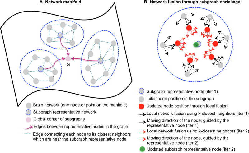
Based on this graph, all brain networks in the manifold can be progressively diffused and fused in accordance to their connected networks, in the direction of the global center as illustrated in Fig. 1.

Fig. 1. Illustration of the proposed manifold-guided diffusive-shrinking graphs for network atlas estimation.

(A) Modeling the manifold of brain networks as a graph partitioned into homogeneous subgraphs, where similar networks are clustered together. (B) Iterative sub-graph shrinking through locally diffusing and fusing each network node with its most similar neighboring nodes, in the direction of the global center of the manifold graph.

• Step 3: Manifold-guided graph shrinkage through diffusion

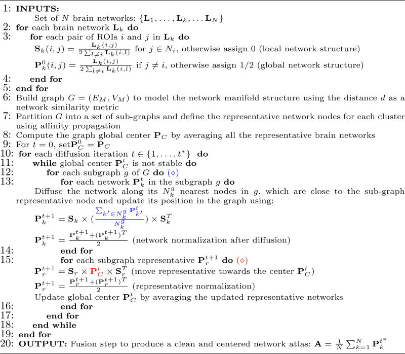
To ensure that the local fusion of each network node with nearby nodes is smooth, we average the representatives of all sub-graphs to generate a center global network. Then, we move each node (i.e., locally update each network) by fusing it with its closest neighboring nodes (i.e., networks) through an iterative process as in [10] in the direction of the global center. Since the representative nodes are moved, we subsequently update the global center. We then repeat these two steps while updating the global center until it becomes stable. Eventually, the as the original graph shrinks where all nodes will locate at the vicinity of the global center P_C, where their averaging is more reliable and meaningful to produce the sought ‘network atlas’ (Fig. 1). The steps for diffusive-shrinking graph for network atlas estimation are detailed in Algorithm 1, where where we denote by the diffusion at a sub-graph level in G and by the diffusion at a higher level in G.

3 Results

Evaluation dataset

We evaluated the proposed framework on 35 typically developing infants, where each subject has 5 serial T1-w, T2-w MRI and resting-state fMRI (rsfMRI) scans acquired at 1, 3, 6, 9 and 12 months of age. We generated two types of brain networks for each subject.

Functional Brain Networks

After rsfMRI pre-processing (including motion correction), we performed infant brain image longitudinal registration from native space to MNI space using GLIRT where each rsfMRI was partitioned into 116 ROIs using AAL template, which includes both cerebral and cerebellar regions. For each subject, we computed the mean fMRI time-series signal in each ROI. Then, we created the 116 × 116 functional connectivity matrix where the connectivity strength between a pair of ROIs represents the correlation between their mean functional signals.

Morphological Brain Networks

After rigid alignment of longitudinal and cross-sectional infant structural MR images (i.e., T1-w and T2-w) and brain tissue segmentation, we reconstructed and parcellated the cortical surfaces into 35 cortical regions using in-house developed tools [12]. By computing the pairwise absolute difference in cortical thickness between pairs of regions of interest, we generate a 35 × 35 morphological connectivity matrix for each time point in each subject.

Evaluation

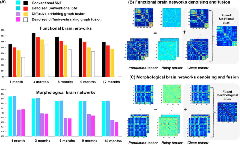
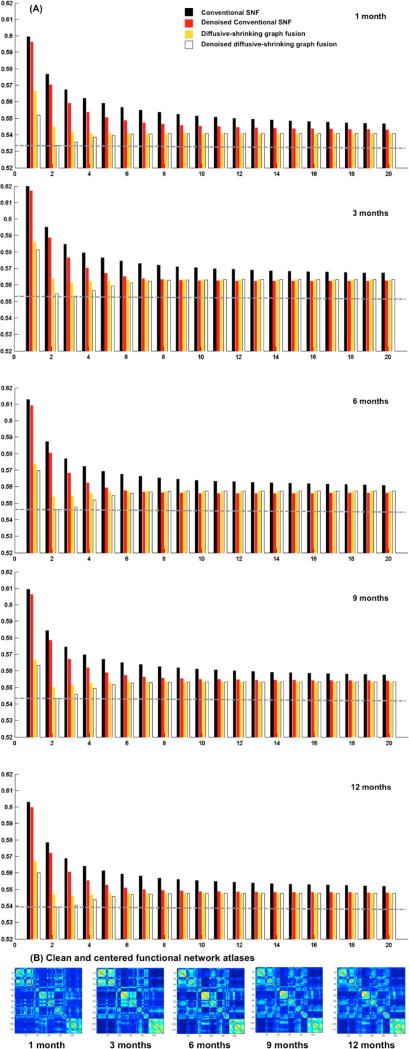
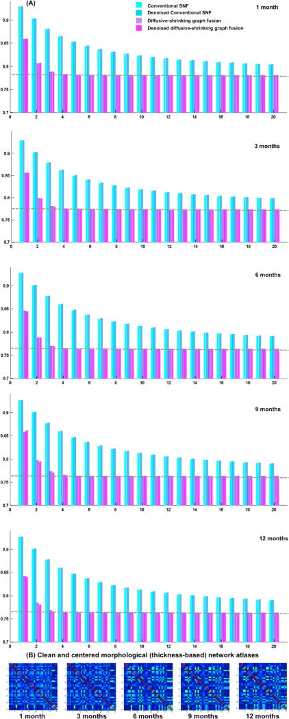
To evaluate the centeredness of the estimated brain network atlas, we compute the mean distance between the estimated network atlas and each individual network in the population using as metric d. Fig. 2 shows the mean distance computed using the proposed network atlas estimation method and the conventional SNF method [9]. The smaller the evaluation distance the more centered is the atlas with respect to the individual networks on the network manifold. We used paired t-test to evaluate the statistical significance of our method in comparison with [9]. Clearly, our method produced more centered network atlases than conventional SNF (p << 0.001) at all acquisition timepoints (Fig. 2). When using functional networks, the denoising step led to more centered network atlases for both our method and SNF (Fig. 2). On the other hand, denoising morphological networks did not further improve the centeredness of the estimated atlases at different timepoints, which can be explained by the fact that fMRI is much noisier than structural T1/T2-w MR imaging. Fig. 3–4 show that at each diffusion iteration, our method generated rapidly a more centered network atlas than the conventional SNF method. Fig. 3-B displays the estimated functional network atlases using our method at different timepoints. A dramatic functional connectivity change occurs between 1 and 3 months of age, followed by a few sparsely distributed changes between 3 and 12 months of age. We also notice that in Fig. 4-B many cortical thickness-based connectivities become weaker (i.e. smaller absolute difference) as we transition from 1 to 3 months of age, which implies that different brain regions develop more similar cortical thicknesses. On the other hand, brighter connectivities appear in morphological network atlases between 3 and 12 months of ages, which shows that the cortical thickness becomes more spatially heterogeneous with age.

Algorithm 1.

Diffusive-shrinking graph strategy for network atlas estimation

Fig. 2. Clean and centered network atlas evaluation.

(A) Mean distance between the estimated network atlas and all individual networks in the population using conventional SNF method and our framework, with and without denoising. (B–C) Network denoising using tensor robust principal component analysis and fusion using the proposed diffusive-shriking graph strategy. We display both functional (B) and morphological (C) estimated network atlases at 9 months of age.

Fig. 3.

(A) Evaluation of the estimated functional network atlases for developing infants (1, 3, 6, 9 and 12 months of age) using the conventional similarity network fusion method introduced in [9] and our proposed diffusive-shrinking graph method. We display the mean distance between estimated network atlas and all individuals in the population of networks at each diffusion iteration, with and without denoising. The dashed gray line shows that our method rapidly achieves the best accuracy within the first diffusion iterations (t* ~ 2). (B) The estimated functional network atlases using our method.

Fig. 4.

(A) Evaluation of the estimated morphological network atlases for developing infants (1, 3, 6, 9 and 12 months of age) using the conventional similarity network fusion method introduced in [10] and our proposed diffusive-shrinking graph method. We display the mean distance between estimated network atlas and all individuals in the population of networks at each diffusion iteration, with and without denoising. The dashed gray line shows that our method rapidly achieves the best accuracy within the first diffusion iterations (t* ~ 4). (B) The estimated morphological network atlases using our method.

4 Discussion and conclusion

We have proposed a diffusive-shrinking graph strategy that follows the local manifold structure of a set of brain networks to gradually fuse them through a diffusion process until reaching the final network atlas. Our results showed that our strategy significantly improves the atlas centeredness and pre-denoising (especially for functional networks) further centers the estimated clean atlases. Additionally, our method converges around 5–10 times faster than the conventional SNF method. While SNF converges when the number of iterations t exceeds 20 as noted in [9], the optimal number of iterations required for our method to converge is t* ~ 2 for functional networks and t* ~ 4 for morphological networks. Precisely, while the SNF mean distance slowly decreases with each diffusion iteration as the atlas becomes more centered (see red and white bars in Fig. 3 and dark blue and pink bars in Fig. 4), our mean distance dramatically drops during the first few iterations (black vs. yellow bars (without denoising) and red vs. white bars (with denoising) in Fig. 3) and then slightly increases and remains stable. This convergence behavior shows first that, following the manifold structure when diffusing, speeds up the convergence process to the optimal t*, and second that over-diffusion t > t* decenters the network atlas as it becomes closer to the identify matrix. Clearly, our method have two advantages over conventional SNF: (1) a better atlas centeredness (shown in Fig. 2-A), and (2) a significantly decreased computational time (shown in Fig. 3–4). We also notice that, when denoising, the diagonals of the denoised tensor may take non- zero values. This is not problematic since the diffusion process automatically resets these values using Eq. 1.

It is worth noting that the proposed network atlas estimation framework is appropriate for large datasets with thousands of networks where the network distribution is complex. Indeed, to capture this complexity, Algorithm 1 can include several hierarchical levels of subgraphs and their representatives that progressively diffuse as they approach the global center of the whole graph. Since our framework overlooks the network distribution in the temporal domain, we will further extend it by enforcing temporal consistency to produce a longitudinal network atlas. Eventually, building clean and centered atlases for healthy individuals as well as patients with a specific brain disease or disorder will help us better identify population-based distinctive changes in brain connectivity, thereby providing reliable features or biomarkers for an accurate diagnosis.

References

- 1.Brown C, Hamarneh G. Machine learning on human connectome data from MRI. arXiv:1611.08699v1. 2016 [Google Scholar]
- 2.Miller K, Alfaro-Almagro F, Bangerter N, Thomas D, et al. Multimodal population brain imaging in the UK Biobank prospective epidemiological study. Nature Neuroscience. 2016;19:1523–1536. doi: 10.1038/nn.4393. [DOI] [PMC free article] [PubMed] [Google Scholar]
- 3.Fallik D. The human connectome project turns to mapping brain development, from birth through early childhood. Neurology Today. 2016;16:7–9. [Google Scholar]
- 4.Glasser M, Coalson T, Robinson E, Hacker CD, et al. A multi-modal parcellation of human cerebral cortex. Nature. 2016;536:171–178. doi: 10.1038/nature18933. [DOI] [PMC free article] [PubMed] [Google Scholar]
- 5.Wassermann D, Mazauric D, Gallardo-Diez G, Deriche R. Extracting the core structural connectivity network: Guaranteeing network connectedness through a graph-theoretical approach. MICCAI. 2016:89–96. [Google Scholar]
- 6.Chen X, Zhang H, Shen D. Ensemble hierarchical high-order functional connectivity networks for MCI classification. MICCAI. 2016:18–25. doi: 10.1007/978-3-319-46723-8_3. [DOI] [PMC free article] [PubMed] [Google Scholar]
- 7.Wu G, Jia H, Wang Q, Shen D. SharpMean: Groupwise registration guided by sharp mean image and tree-based registration. NeuroImage. 2011;56:1968–1981. doi: 10.1016/j.neuroimage.2011.03.050. [DOI] [PMC free article] [PubMed] [Google Scholar]
- 8.Lu C, Feng J, Chen Y, Liu W, et al. Tensor Robust Principal Component Analysis: Exact recovery of corrupted low-rank tensors via convex optimization. CVPR. 2016:5249–5257. [Google Scholar]
- 9.Wang B, Mezlini A, Demir F, Fiume M, et al. Similarity network fusion for aggregating data types on a genomic scale. Nat Methods. 2014;11:333–337. doi: 10.1038/nmeth.2810. [DOI] [PubMed] [Google Scholar]
- 10.Ying S, Wu G, Wang Q, Shen D. Hierarchical unbiased graph shrinkage (HUGS): a novel groupwise registration for large data set. Neuroimage. 2014;1:626–38. doi: 10.1016/j.neuroimage.2013.09.023. [DOI] [PMC free article] [PubMed] [Google Scholar]
- 11.Frey B, Dueck D. Clustering by passing messages between data points. Science. 2007;315:972–976. doi: 10.1126/science.1136800. [DOI] [PubMed] [Google Scholar]
- 12.Li G, Wang L, Shi F, W L, et al. Simultaneous and consistent labeling of longitudinal dynamic developing cortical surfaces in infants. Med Image Anal. 2014;18:1274–1289. doi: 10.1016/j.media.2014.06.007. [DOI] [PMC free article] [PubMed] [Google Scholar]