Population stress: A spatiotemporal analysis of population change and land development at the county level in the contiguous United States, 2001–2011

Abstract

The past century has witnessed rapidly increasing population-land conflicts due to exponential population growth and its many consequences. Although the measures of population-land conflicts are many, there lacks a model that appropriately considers both the social and physical contexts of population-land conflicts. In this study we introduce the concept of population stress, which identifies areas with populations growing faster than the lands available for sustainable development. Specifically, population stress areas are identified by comparing population growth and land development as measured by land developability in the contiguous United States from 2001 to 2011. Our approach is based on a combination of spatial multicriteria analysis, zonal statistics, and spatiotemporal modeling. We found that the population growth of a county is associated with the decrease of land developability, along with the spatial influences of surrounding counties. The Midwest and the traditional “Deep South” counties would have less population stress with future land development, whereas the Southeast Coast, Washington State, Northern Texas, and the Southwest would face more stress due to population growth that is faster than the loss of suitable lands for development. The factors contributing to population stress may differ from place to place. Our population stress concept is useful and innovative for understanding population stress due to land development and can be applied to other regions as well as global research. It can act as a basis towards developing coherent sustainable land use policies. Coordination among local governments and across different levels of governments in the twenty-first century is a must for effective land use planning.

1. Introduction

The global population exponentially increased throughout the twentieth century. The estimated global population in 2016 was approximately 7.4 billion and is expected to increase to 9.6 billion in 2100 (Gerland et al., 2014). Population growth has been documented as a social and environmental issue. Under the condition of limited resources, regional population growth can induce severe community vulnerabilities (Neumann et al., 2015) such as water scarcity (Falkenmark, 2013), livestock and food insecurities (Godber & Wall, 2014), and burdens on health care (Dall et al., 2013). Population growth and redistribution, however, is constrained by land development and conversion, and in a trade-off relationship they collectively affect community vulnerability (Chi, 2010a). The nexus of population, land, and community vulnerability is covered in a large body of literature of population-land conflicts. Such conflicts include hot spots in wildfire-urban interfaces, coastal and flooding areas, exurban areas, ecosystem areas around national parks, declining urban areas, abandoned rural lands, and others.

1.1. Quantifying population-land conflicts

How are population-land conflicts quantified and measured in existing research? Although population-land conflicts involve both social and physical contexts, unfortunately existing research measures either social or physical contexts rather than both. The social context of population-land conflicts is determined by multiple social or socioeconomic subcomponents, such as legal regulation (Grout, Jaeger, & Plantinga, 2011; Lestrelin, Castella, & Bourgoin, 2012), social/environmental policy (Lambin et al., 2014), economic values of lands (Lambin & Meyfroidt, 2010), and social networks (Barton, 2009; Marull, Pino, Tello, & Cordobilla, 2010). These subcomponents under the social context are, however, more ontological and theoretical and cannot be directly measured by the sizes of lands. In order to determine the change of land through a social context, traditional studies such as political ecology research have generally applied “metabolism” to define the critical point of land change through policy (Gandy, 2004; Marull et al., 2010) or the concept of “hybridity” to identify the socioenvironmental modification from multiple backward and forward changes through political decisions and social movements (Brownill & Carpenter, 2009; Forsyth, 1996; Holman & Rydin, 2013; Qureshi & Haase, 2014). Moving toward mathematical modelling, Kennedy, Pinceti, and Bunje (2011) reviewed over 50 articles related to urban metabolism and environmental assessments and found that using urban metabolism as a model framework can integrate social sciences and biophysical sciences. It can also help analyze policy and technology outcomes to achieve sustainability goals. However, most studies integrating mathematical modelling also indicated the focus of “urban metabolism” has shifted from a critical point of land change through policy to a critical point of land change through time. Because of this shift of focus, most quantitative-based urban metabolism models can provide results for policy decision making but cannot include elements of land policies or governmental regulations during the modelling process. However, recent reviews of political ecology (Angelo & Wachsmuth, 2015; Gandy, 2015; Sharma-Wallace, 2016) indicate that most studies of metabolism and hybridity were qualitative based without using any mathematical or statistical modelling techniques.

In contrast, the physical context of population-land conflicts is determined by quantifying the geophysical environment, for example, estimating sizes and amounts of each land type. Previous studies researching physical contexts include using geographic information system (GIS) and remote sensing techniques and land use and land cover (LULC) to predict land use changes (Alexakis et al., 2014; El-Kawy, Rød, Ismail, & Suliman, 2011; Hu & Wang, 2013; Ye, Zhang, Liu, & Wu, 2013) or using global environmental modelling techniques such as the Community Earth System Model (CESM), Global Land-use Model (GLM), or Global Change Assessment Model (GCAM) to quantify the land cover and to estimate future simulations (Chen & Dirmeyer, 2016; Di Vittorio et al., 2014). These techniques provide the results of net change of land cover or frequencies of land changes in a study period, without considering the influences of land policies or governmental regulations for development. One common example is that LULC analyses can involve stochastic statistical modelling or complex economic modelling for spatiotemporal assessment, such as the Markov model (Halmy, Gessler, Hicke, & Salem, 2015; Singh, Mustak, Srivastava, Szabó, & Islam, 2015; Xu & Huang, 2014), but land policies were not the factors of such models.

In summary, previous population-land studies linked to the social context of land use and development focused on hypothetically defining the land without quantitative assessments, while most studies linked to the physical context reported only land change by statistical modelling without fully considering the socioeconomic values or the sociopolitical issues of lands. This reveals, therefore, a gap in the knowledge of how to combine both the social context and the physical context to develop a quantitative model for appropriately estimating population-land relationship and identifying hot spots of population-land conflicts.

1.2. Population stress

To consider both the social and physical contexts for defining and quantifying population-land relationships, we introduce in this study a concept called population stress. We define population stress as an area that experiences faster population growth than land development. Such areas often experience high-density development. They need more resources than an average developing area to support the increased population. This creates higher demands on food, water, energy, and infrastructure. Such areas, in turn, experience higher “stress” than an average developing area.

But why is population growth an appropriate indicator of the social context of population-land conflicts? After all, the social context has many elements, including social, economic, demographic, and policy elements; and community vulnerability is affected not only by population growth but also its consequences. That said, we argue that population growth is a reasonable indicator (and probably the best indicator) to represent the overall social context because regional population change is a spatiotemporal dynamic flow between demographic characteristics, socioeconomic conditions, infrastructure, the natural environment, and land use and development (Chi & Ventura, 2011), and population change is found to be associated with over 80 factors in these domains (Chi, 2009). It should be noted that population growth is not the only indicator, and not always the best indicator, to represent the social context of population-land conflicts. Depending upon the specific population-land conflict, a different indicator could be better suited to social context. For example, if inequality is the focus of a population-land conflict study, socioeconomic statuses (e.g., race/ethnicity, income, and education) might be better indicators of the social context. Our focus in this study is to identify hot spots of areas that experience population stress, that is, population growth faster than land development. For this purpose, population growth is a reasonable indicator of the social context of population-land conflicts.

1.3. Land developability

Our population stress measure is essentially a comparison between population growth and land development. While population growth is easy to calculate, land development can be measured in a variety of ways, as discussed previously. In order to measure land development in relation to population change with consideration of both social and physical contexts, a conceptual idea called “land developability” would be an appropriate measure (Chi, 2010a). The concept of land developability is to quantify the availability for land development in a particular region based on spatial information of both social and geophysical factors, including 1) federal restriction, 2) environmental risk, and 3) urban structure. By making use of the component of spatial heterogeneity, this index could 1) be used to develop a spatiotemporal model for analyzing socioenvironmental impacts on population change and 2) correlate with socioeconomic factors such as transportation (Chi, 2010b; Chi, 2012), deforestation (Clement, Chi, & Ho, 2015), and natural amenities (Chi & Marcouiller, 2013a) for further demographic assessment. In contrast to common land vulnerability indices that only indicate the negative impacts of land development for environmental risk assessment, the land developability index can demonstrate both the positive and negative sides of land development, resulting in a balanced judgement of land conversion for the use of determining regional population dynamics. Analyzing population dynamics alongside land developability will not only be an application of regional planning but is also essential for predicting spatial demographic trends, economic geographic patterns, and sociodemographic changes through spatiotemporal modelling.

Reviewing the previous studies that have applied the land developability index in modeling, we found that most studies focused on a relatively small geographic extent, such as counties within a state (Chi, 2010b; Chi, 2012; Chi & Marcouiller, 2013a). There is a lack of research interpreting the relationship between land developability and population change in a greater region (e.g., the contiguous United States). This missing interpretation is the key to reducing the socioenvironmental vulnerability of a country and to enhancing population forecasting in a national context. Within the context of rapid urban sprawl and rural development in the twenty-first century, the land developability index can be useful for analyzing regional/national population change in order to 1) locate areas with less stress for migration and 2) locate regions that may need to change their corresponding land types for sustainable development (e.g., change urban lands to green cities).

We hereby develop the first national study to investigate the relationship between land developability and population change with a spatiotemporal approach. We selected the contiguous United States as our study site because it has faced substantial changes in terms of population and land use in the past decades. In an aspect of regional scale, the changes of landscape can be a driving force of national mitigation (aka population change), and this population change can further influence the demographic characteristics at a local scale, such as inequality and income increase. The overarching objective of this study is to develop a regional/national protocol for identifying population stress areas by considering the social and physical contexts of land development that can also apply to other countries or continents with similar data sets in the future. We have three specific goals: 1) to map the land developability from 2001 to 2011 at the county-level scale, 2) to analyze the spatiotemporal relationship between land developability change and population change, and 3) to identify population stress areas by locating the spatial clusters with significant changes in land developability and population. The contributions of our method are: 1) the ability to quantify the population stress from land development of each county in the contiguous United States over time and 2) the ability to identify the counties or regions with higher or lower population stresses from land development over time and across space.

2. Five key elements of land developability

We make a simple assumption that the following five types of lands are the areas that are not suitable for future development: 1) surface water, 2) steep slope, 3) built-up land, 4) wetland and protected wildlife area, and 5) tax-exempted land (federal- and state-owned land).

Surface water, including rivers, lakes, and oceans, is not suitable for land development. There are issues related to legal matters and practical matters (Albert, Lishman, & Saxena, 2013), ecosystem protection and restoration (Harrison et al., 2016; Martinuzzi et al., 2014), and natural hazard risk such as flooding (Jongman, Ward, & Aerts, 2012; Ludy & Kondolf, 2012). To identify the areas of the contiguous United States associated with surface water, we applied the 2001 and 2011 National Land Cover Data (NLCD) from Multi-Resolution Land Characteristics Consortium and U.S. Geological Survey (USGS), as shown in Table 1. The NLCD were derived from Landsat images (Homer, Huang, Yan, Wylie, & Coan, 2004; Homer et al., 2007; Homer et al., 2015) and converted to a land use classification scheme with eight major classes. Surface water of our study is identified based on “open water” under the “water” class of NLCD, which indicates areas with less than 25% coverage of vegetation and soils within an approximately 30 m radius.

Table 1.

Spatial data sets for locating five major types of undevelopable lands

Data set	Type of land	Data type	Ground sample size	Acquisition date	Source
National Land Cover Data (NLCD)	Surface water, built-up land, wetland	Raster	30 m	2001 and 2011	Multi-Resolution Land Characteristics Consortium
Federal and Indian Lands	Tax-exempted land (federal- and state-owned land)	Vector (polygon)	–	2000	U.S. Geological Survey
Managed Areas Database (MAD)	Wetland and protected wildlife area, tax-exempted land (federal- and state-owned land)	Vector (polygon)	–	1996	Remote Sensing Research Unit, University of California-Santa Barbara
Shuttle Radar Topography Mission (SRTM) Version 4 Digital Elevation Model (DEM)	Steep slope	Raster	90 m	2000	Consultative Group on International Agricultural Research-Consortium for Spatial Information (CGIAR-CSI)
Cartography boundary files	County boundary	Vector (polygon)	–	2010	U.S. Census Bureau

Steep slope, mainly areas with slopes >=20%, are not suitable for land development (Wang, Yu, & Huang, 2004). Soils and bedrock at such areas are relatively unstable and have a higher probability of natural hazard occurrences such as landslides (Imaizumi, Sidle, Togari-Ohta, & Shimamura, 2015; Liu, Nearing, & Risse, 1994; Zhou, Fang, & Liu, 2015). As a result, urban development on these landforms may cause property damage and loss of human life (He & Beighley, 2008). In addition, there are legal requirements, such as Wisconsin’s Erosion Control and Stormwater Management Ordinance of 2002, restricting development on such landscapes (Chi, 2010a). We identified areas with slopes >=20% based on the Shuttle Radar Topography Mission (SRTM) Version 4 Digital Elevation Model (DEM) from the Consultative Group on International Agricultural Research–Consortium for Spatial Information (CGIAR-CSI) (Jarvis, Reuter, Nelson, & Guevara, 2008). SRTM is an elevation data set with 3-arc seconds resolution (approximated 90 m at equator) originally built by the Jet Propulsion Laboratory of the California Institute of Technology and National Aeronautics and Space Administration (NASA). The original data of the data set were collected in February 2000 from a specific modified radar system in an 11-day satellite mission. SRTM version 4 was modified as a hole-filled DEM by the void-filling interpolation method (Reuter, Nelson, & Jarvis, 2007). We reclassify slope into two classes for spatially delineating the areas with gentle slopes and steep slopes: <20% and >=20%.

Areas with high percentages of built-up land are likewise not suitable for further development. It has been recognized that a dense built environment leads to significant environmental issues such as poor air quality (Ng, 2009; Yim, Fung, Lau, & Kot, 2009). High percentages of socioeconomically deprived populations in dense built environments can result in higher health risks (Sariaslan et al., 2014) unless sustainable policies for urban transformation are applied to such neighborhoods. We identified built-up land based on NLCD. The definition of built-up land for this study is an area (approximately 30 m radius) with 20% or more impervious surfaces, where we can commonly find single/multi-family houses, apartments, townhouses, and other commercial/industrial properties (Chi, 2010a).

Wetland is not suitable for land development because it is an important environmental resource that can serve as a diverse ecosystem (de Groot et al., 2012; Russi et al., 2013), a carbon sink (Bernal & Mitsch, 2012; Doughty et al., 2016; Mitsch et al., 2013), and a natural purifier of water and air pollution (Greenway, 2004; Zhang, Xu, He, Zhang, & Wu, 2012; Zhu et al., 2016). Recent studies also indicate that loss of wetland can induce higher soil erosion risk and vulnerability to drought (Ockenden, Deasy, Quinton, Surridge, & Stoate, 2014; Wright & Wimberly, 2013). Protected wildlife areas are areas designated for federal conservation or state protection of endangered species, protected species, and other lives or activities (Watson, Dudley, Segan, & Hockings, 2014). Legal regulations and land policies apply to protected wildlife areas for constraining land development in order to protect ecological systems (Chi, 2010a; Worboys, Lockwood, Kothari, Feary, & Pulsford, 2015). Previous research indicates that inappropriate land use (i.e., development of wetland and protected wildlife areas) has induced a great loss of global ecosystem services up to 4.3–20.2 trillion USD per year (Costanza et al., 2014). Therefore, both wetland and protected wildlife areas are defined as “undevelopable” areas in this study. In order to identify the wetland and protected wildlife areas, we combined NLCD, USGS’s Federal and Indian Lands map, and University of California–Santa Barbara’s Managed Areas Database (MAD) to locate the associated regions. The USGS Federal and Indian Lands map is a spatial data set created by the U.S. Geological Survey in October 2000 that contains information of 1) tax-exempted federal and state lands and 2) national and state protection areas. MAD is a spatial database that contains information of national managed areas, state managed areas, Indian and military reservations, and wilderness areas (McGhie, Scepan, & Estes, 1996). “Woody wetlands” and “emergent herbaceous wetlands” from NLCD are identified as wetlands for land developability mapping. “Wilderness,” “Wilderness Study Area,” and “Wildlife Management Area” from the USGS Federal and Indian Lands map and “Wilderness,” “Wilderness Study Area,” and “Wild and Scenic Area” from MAD are identified as protected wildlife areas.

Tax-exempted land such as federal- and state-owned lands are legally protected and publicly owned. These lands are restricted for residential, commercial, or other-purpose land development (Chi, 2010a). All forests, parks, trails, wildlife refuges, fishery areas, and other areas indicated as being federally owned or state owned based on the USGS Federal and Indians Lands map and MAD are identified as tax-exempted land for land developability mapping.

3. Methods

3.1. Land developability of United States in 2001 and 2011

The land developability of the United States in 2001 and 2011 is measured based on the results of spatial multicriteria analysis (SMCA) and zonal statistics, with five key elements (Table 1) previously stated:

• surface water,

• steep slope,

• built-up land,

• wetland and protected wildlife area, and

• tax-exempted land.

SMCA is a common statistical method used for environmental vulnerability estimation (Aubrecht & Özceylan; 2013; Chang & Chao 2012; Huang, Keisler, & Linkov, 2011; Ho, Knudby, & Huang, 2015) that combines spatial data sets in an analysis by assigning a specific weight to each data set based on its importance to vulnerability. An equal weight/additive approach is applied to this SMCA for avoiding subjectivity of index development based on the guideline of the United Nations Environment Programme (2002).

SMCA is conducted based on the following steps: 1) spatial data sets of five types of undevelopable lands are first converted to binary raster layers with 90 m resolution, where a “1” in a pixel on these binary maps indicates an area with undevelopable land and a “0” indicates an area that is conceptually developable; 2) these five spatial layers are overlaid, and the sum of all the layers for each pixel is calculated; and 3) the areas with values >=1 are reclassified as “1” and these areas are indicated as undeveloped lands, the areas with values equal to 0 are reclassified as “0” and identified as developable. This new binary map is then used for zonal statistics to calculate the percentage of land developability in each county.

For estimating the percentage of land available for future development and conversion, the areas with values of “0” (the areas identified as developable lands) are changed to “100” to represent 100% of land developability within a 90 m pixel, while the areas with “1” (the areas identified as undevelopable) are converted to “0” to represent 0% of land developability within a pixel. Zonal statistics is then used to average the values of all pixels within a given county boundary. This procedure is applied to each county across the United States, in 2001 and 2011, separately, to estimate the land developability.

3.2. Estimating the spatiotemporal impact of land developability change on population change

We estimate the spatiotemporal impact of land developability change on population change from 2001 to 2011 at the county level based on three sets of regressions: an ordinary least squares (OLS) regression, three spatial regression models (spatial lag model, spatial error model, and spatial error model with lag dependence), and a geographically weighed regression (GWR). County-level population data were retrieved from the 2000 and the 2010 U.S. Censuses. OLS regression is used to determine the association that population has with land developability without considering spatial influences from neighboring counties. The three spatial regression models consider the spatial influences in the forms of spatial lag and/or spatial error terms (Chi & Zhu, 2008). The GWR is a different type of spatial regression model that examines whether spatial heterogeneity is observed in the relationship between the dependent variable and independent variables of a study (Brunsdon, Fotheringham, & Charlton, 1998; Fotheringham, Brunsdon, & Charlton, 2003). It should be noted that the GWR is used mostly as an exploratory tool for illustration purposes (Videras, 2014).

In this study, the percentage of population change is assigned as the dependent variable for OLS regression and GWR and is calculated as follows:

$$\text{Percentage}\text{of}\text{Population}\text{Change}=\frac{(2011\mathit{population}-2001\mathit{population})}{2001\mathit{population}}\times 100$$

The change of land developability is assigned as the independent variable of all regressions and is calculated as follows:

$$\text{Land}\text{Developability}\text{Change}=2011\mathit{Land}\mathit{Developability}(\%)-2001\mathit{Land}\mathit{Developability}(\%)$$

OLS regression and spatial regression models are conducted in GeoDa. GWR is conducted based on the ArcTool function in ArcGIS 10.3.

3.3. Identifying population stress areas

We also apply a differential local Moran’s I analysis implemented in GeoDa software (Anselin, Syabri, & Kho, 2006) to identify the statistically significant clusters with hypothetically higher population growth than hypothetically higher land developability decreases. Local Moran’s I analysis is commonly used to estimate the spatial autocorrelation between neighboring features (Anselin, 1995). Spatial weight is defined using the k-nearest neighbors (KNN) algorithm with four spatial neighbors. KNN is an asymmetrical spatial-weighting method (Getis & Aldstadt, 2010) and is particularly useful for spatial features with different sizes, such as counties. It ensures that the same number of nearby spatial features is used in all calculations, independent of the total number and size of spatial neighbors.

For the differential local Moran’s I analysis, we compared the percentage of population change to the percentage of land developability change. “High-high” clusters on the local indicators of spatial association (LISA) map indicate spatial clusters of counties with magnitudes of population growth stronger than land developability decline. In other words, the spatial clusters indicate counties with hypothetically >1% increase of population under the condition of potentially 1% decline of land developability of each county. In contrast, “low-low” clusters indicate areas with magnitudes of population growth weaker than land developability decline over a 10-year period, which also means that in a hypothetically 1% decrease of land developability, there would be less than 1% population growth within the spatial cluster.

4. Results

4.1. Land developability of United States in 2001 and 2011

In general, the West Coast, the Great Lakes area, and Florida have the lowest land developability and the Midwest and the South are the areas with the highest land developability (Figure 1). However, there are also fair amounts of low-land-developability counties next to high-land-developability counties in the Midwest, while Central Valley in California shows higher land developability compared to other regions in the West, which generally indicate low developability.

Figure 1.

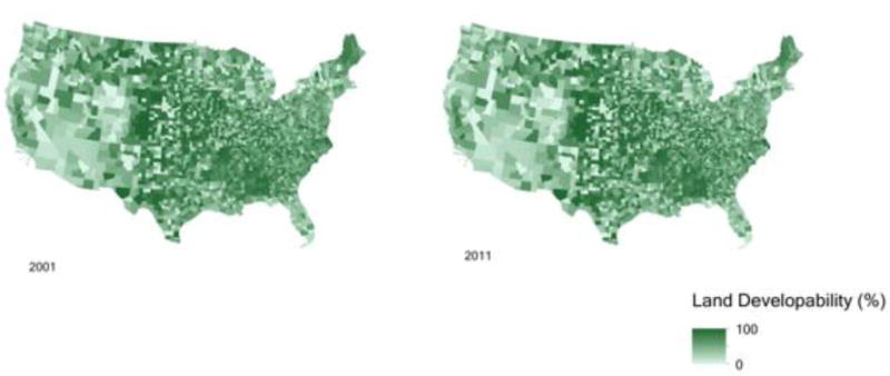
Land developability across the United States in 2001 and 2011. Lighter green indicates lower land developability within a county and darker green indicates higher land developability.

Among all counties across the contiguous United States, the majority of them had significant decreases in land developability from 2001 to 2011 (Figure 2): 72.1% of counties had 0% to 5% decreases in land developability, 9.4% of counties had 5% to 15% decreases, and 1.4% of counties had >15% decreases. Counties with higher land developability decreases (>=5%) were more likely located on the East Coast. There were also several isolated counties with land developability increases (>0%) in the Midwest and the South, and one isolated county had more than a 15% increase of land developability from 2001 to 2011, probably due to dropping percentages of built-up lands from more than 20% impervious surfaces to less than 20% impervious surfaces over these 10 years.

Figure 2.

Change of land developability from 2001 to 2011 in each county of the contiguous United States.

4.2. Spatiotemporal change of population change and land developability between 2001 and 2011

Without considering the spatial influences of neighboring counties, the result of the OLS regression showed a negative effect of land developability change on population growth from 2001 to 2011; and the negative effect is statistically significant at the p <= 0.001 level (Table 2). This means that population growth is associated with a decline in land developability. The diagnostics for spatial dependence indicated that there are statistically significant spatial lag and spatial error terms remaining in the model residuals, suggesting that spatial regression models dealing with the spatial dependence should be fitted to the data. Measures of fit indicated that all three spatial regression models were better fitted to data than the OLS model, and the spatial error model with lag dependence triumphed over all other models.

Table 2.

Regression results

	Ordinary least squares regression	Spatial lag model	Spatial error model	Spatial error model with lag dependence
Constant	4 75*** (0.26)	1.53*** (0.23)	4.78*** (0.54)	−0.22 (0.14)
Land developability change	−0.26*** (0.06)	−0.14** (0.05)	−0.08 (0.05)	−0.10** (0.04)
Spatial lag term	/	0.64*** (0.02)	/	1.00*** (0.01)
Spatial error term	/	/	0.64*** (0.02)	−0.62*** (0.03)
Diagnostics for spatial dependence
Moran’s I	0.42***
LM (lag)	1451.08***
Robust LM (lag)	32.98***
LM (error)	1426.22***
Robust LM (error)	8.12**
LM (lag and error)	1459.20***
Measures of fit
Log likelihood	−12,406	−11,888	−11,893	−11,537
AIC	24,815	23,783	23,789	23,079
BIC	24,827	23,801	23,801	23,097
N	3,108	3,108	3,108	3,108

Notes:

^***p ≤ 0.001,

^**p ≤ 0.01,

^*p ≤0.05; standard errors are in parentheses.

LM = Lagrange Multiplier. AIC = Akaike information criterion. BIC = Schwartz’s Bayesian information criterion.

A larger log-likelihood value or a smaller AIC/BIC value suggests that the model is better fitted to data. Overall, the measures of fit indicate that the spatial error model with lag dependence is best fitted to data.

According the results of the spatial error model with lag dependence, population change has a negative association with land developability change. For each 1% decrease in land developability, population grows 0.1%. On average, a county’s population grows 1% for each 1% growth in its neighboring counties’ populations.

The OLS and spatial regression models produced “global” coefficients where the effect of an independent variable on the dependent variable is fixed. The effect, however, could vary spatially from one county to another due to the possibly different local contexts. The GWR can produce locally varying coefficients. According to the GWR results, only 0.3% of counties were extremely underestimated and with standard deviation residuals lower than −2.5 and only 2.6% of counties were extremely overestimated and with standard deviation residuals greater than 2.5. In contrast, 51.6% of the total counties had standard deviation residuals >= −0.5 and <= 0.5, indicating relatively accurate prediction from the GWR model and implying that the decrease of the amount of lands available for development in the contiguous United States could actually affect the population growth.

Among all counties in the contiguous United States, we found significant clusters with more than a 1% increase in population growth in a 1% decrease of land developability only on the coast of California and in greater Miami, greater Las Vegas, and greater Minneapolis (Figure 3). Other areas on the West Coast and in the Midwest, Florida, and New England had slight population growth (less than 1%) in a 1% decrease of land developability, indicating that population grew more slowly than the decrease of land developability. Compared to these areas, other counties in the United States showed a positive relationship between population growth and land developability change. In South Texas, the greater St. Louis area, North Georgia, Central Pennsylvania, and the Central Valley of California, a 1% decrease of land developability was associated with more than a 1% decline in population.

Figure 3.

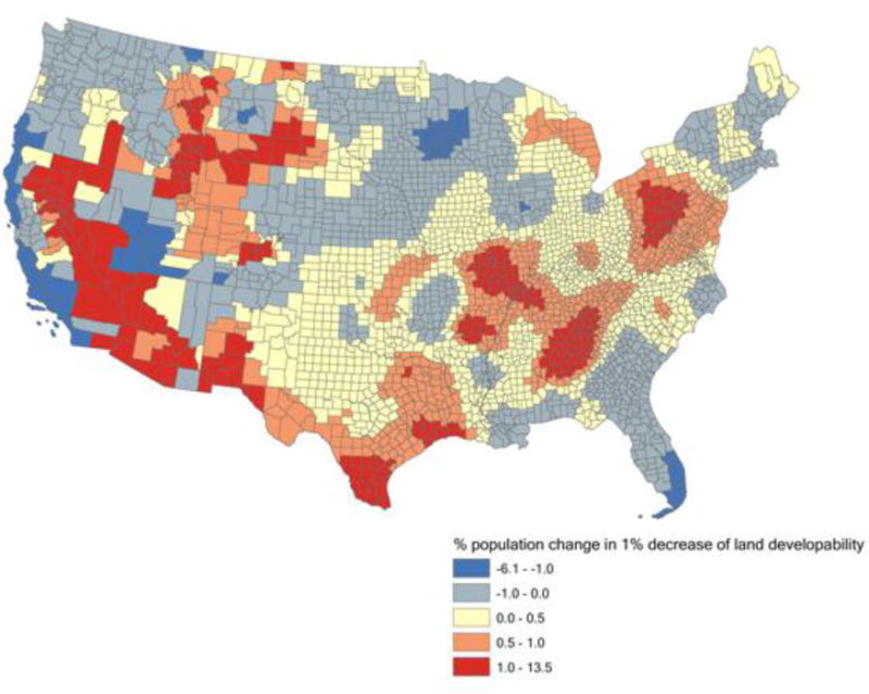
Coefficient of geographically weighted regression (GWR). Results indicate the percentage increase in population associated with a 1% decrease in land developability of each county in the contiguous United States. Red indicates counties with faster increases of population than the decline of land developability, and blue indicates slower population growth than the decline of land developability of a county.

4.3. Population stress areas

Global results of differential Moran’s I analysis (Moran’s I: 0.42) indicated that there was a general trend of spatial autocorrelation, with spatial clusters of population growth faster than land developability decrease or population decline slower than land developability increase in the contiguous United States.

Among all counties in the contiguous United States, 8.7% of them indicated “high-high” spatial clusters, including areas on the Southeastern coast and in Washington State, North Texas, and large areas of the Southwestern United States (Figure 4). These are the hot spots with population growth faster than land developability decreases. In contrast, 12.1% of counties in the contiguous United States had “low-low” clusters, including areas of the Midwest, the Great Lakes area, northeastern Mississippi, and northern Alabama. They are areas where population grew more slowly than land developability decreases. In other words, further development in “low-low” clustered areas such as the Midwest would have fewer population issues in sharing available land or land resources in the future, while development in “high-high” clustered areas will be limited by the available and developable lands and the current population trends.

Figure 4.

Spatial correlation of Moran’s I results. High-high clusters (red) indicate spatial clusters of areas with hypothetically 1% loss of land developability having more than 1% population growth, that is, population stress areas. Low-low clusters (blue) indicate spatial clusters of areas with hypothetically 1% loss of land developability having less than 1% population growth.

Discussion and conclusion

5.1. Interpretation of findings

In this study we introduced the population stress concept to identify areas where population grows faster than the lands available for sustainable development. We did this by comparing population change to land development, with the latter being measured by land developability (Chi, 2010a). We analyzed the spatiotemporal impact of land developability change on population change from 2001 to 2011. We applied differential local Moran’s I analysis to estimate relative increases in population in 1% hypothetical increases in land developability in order to analyze the population issues in relation to available land resources in the future. It is also important to note that the “high-high” spatiotemporal clusters from the differential local Moran’s I analysis indicated either 1) population grew faster than the decline of land developability or 2) population decreased more slowly than the increase in land developability. The relative increase of population compared to a 1% hypothetical increase of land developability was only conducted to normalize the data so that we could identify whether the counties may face issues of land development in terms of both population change and land developability change under the current population trend from a period of 10 years. This approach is developed with the understanding that land developability is more likely to decrease under the urbanization in a maturely developed country, such as the United States.

We found that the population growth of a county is associated with its decrease of land developability in the contiguous United States, along with the spatial influences of surrounding counties. We also found that the Midwest and the traditional “Deep South” counties would have less population stress with future land development. The Midwest “rusty belt” has been losing population due to the declining manufacturing industry (Winkler & Johnson, 2016). The “Deep South” is a region characterized as rural, predominantly black, and with high poverty and unemployment (Wimberley & Morris, 2002). In contrast, the Southeast Coast, Washington State, Northern Texas, and the Southwest would face more stress due to population growth and the loss of suitable lands for development. These areas have experienced rapid population growth as they are desirable places to live—with abundant employment opportunities; well developed public infrastructure, healthcare facilities, and education; and/or easy accessibility to work (Chi, 2017). The factors contributing to population stress may differ from place to place because they may have different local contexts (Chi & Marcouiller, 2013b). This needs further investigation in future research.

An advantage of using this method is that we can identify areas that may still be able to have further land development, not only by the amount of available lands but also considering the population trend. However, this model is more suitable for comparing land developability change than for sustainability planning. For example, the Midwest actually had a 0% to 5% decrease of land developability in general, yet the population decline of the Midwest was extremely high—some counties had a >40% decrease of population within 10 years. Those areas showed relatively fewer issues of development on available lands under the current population trend, while at the same time land developability was decreasing. Future investigation could emphasize the magnitude of vulnerability to develop a better scheme of sustainable planning.

Another advantage of our study is that we developed a protocol that can investigate population dynamics in terms of population change, the natural environment, and land use and development with a spatiotemporal approach. The results show the ability of using spatial demographic models to describe population change on a regional scale while at the same time indicating the importance of including spatial factors, by comparing results from aspatial and spatial models. The current research provides insights into why and how we should do it in order to measure population dynamics appropriately. For future study, stratifying the urban–rural continuum (Chi & Marcouiller, 2013a) and population subgroups (e.g., the elderly, non-married, number of households) may provide a greater picture of population dynamics at a finer scale.

5.2. Policy implications

There are several practical uses of the combined population stress concept and land developability index for future planning and policy making. One is that it will enable more straightforward understanding of available lands with the land developability index because it clearly indicates the lands that are suitable or unsuitable for future development. With this knowledge, planners and policy makers can identify areas that may be at risk from increasing population and declining land developability. Pinpointing such at-risk areas clarifies where it is most necessary to undertake interventions in the built environment that can increase the quality of life and alleviate the pressures that come with population stress. Such interventions include sustainable planning protocols such as increasing community features (e.g., health facilities) to reduce social burdens as well as urban planning protocols such as mandating more air ventilation and higher amounts of greenery to create better geophysical environments for residents. It has been widely studied that such communities with better social and physical environments can improve the perceived health of a population (Wong, Yu, & Woo, 2017).

Additionally, the land developability index can act as a guide to help develop land use policies that ensure that urbanization does not lead to further social or environmental pressures. Combining this index with population data can indicate the negative effects of urban growth on land development as well as potential pressures on natural resources (indicated by the loss of carbon sinks and biodiversity, groundwater loss, and deforestation). With this knowledge, land policies can be developed to avoid potential urban metabolism issues that increase environmental deprivation in the future. How could undevelopable or decaying lands within cities be better utilized to serve an increasing population? Could a declining population and large open/developable lands put pressures on the local government through declining tax revenues but increasing infrastructure burdens? These are potential planning questions that our population stress concept and the land developability index could shed light on.

It should be noted that land use planning in response to population change versus land development should not be the responsibility of individual local governments. Rather, land use planning could be better done in coordination with neighboring local governments, as well as upper administration levels such as states and the federal government. Our spatial regression and GWR results indicated that there are strong spatial spillover effects of population change as well as spatial variations of the relationship between population change and land development. Our world has become more connected due to the development of transportation infrastructure and innovations in communication tools. What happens in one place could easily impact its neighboring places (Chi & Marcouiller, 2013b). Coordination among local governments and across different levels of governments in the twenty-first century is a must for effective land use planning.

5.3. Limitations and future directions

We used the county level as the spatial scale of this study because the state level is too coarse to describe regional change in detail but subcounty levels, such as the census-tract level, may require more factors (and thus more data) that can affect local or regional population dynamics. For future study of investigating fine-scale population dynamics as stated previously (e.g., the urban-rural continuum), we recommend using census-tract-level data or a combination of data with different spatial scales (e.g., state, county, and census-tract levels) in order to develop a comprehensive spatial model for predictions. This will provide greater ability to describe macro-scale, mesoscale, and micro-scale regional changes and, at the same time, maintain the accuracy of the prediction. We also recommend that more socioenvironmental factors be considered in the future models, for example, transportation infrastructure, socioeconomic conditions, and natural amenities. Although this adjustment may increase the complexity of the models, it can also provide a better understanding of actual population dynamics in a fine-spatial-scale change. These results will therefore be more useful for future regional planning at both large and small spatial scales.

It should be noted that our land developability index is produced on the basis of only five data layers with simple assumptions. The index should be refined in future research by 1) considering elements of land fragility, vulnerability, and developmental limitations with an eye toward long-term land sustainability and replenishment, and 2) studying and weighting regional variations of the perceptions of relevant factors. For example, mountain views are appreciated more in the American West than in the rest of the United States; therefore, mountain views should be weighted differently in different parts of the country. In order to create a varying weight for each factor, multidisciplinary research will be conducted to link each factor to population change. More broadly, land developability can be linked to population change for identifying hot spots of population-environment conflicts, including wildfire-urban interfaces, coastal and flooding areas, exurban areas, ecosystem areas around national parks, declining urban areas, and others. This will provide significant insights for making efficient and effective policies to tackle the complexity of population-environment conflicts.

Highlights.

• Population stress areas refers to those with populations growing faster than the available lands.

• Population growth is associated with the decrease of land developability.

• Low population stress is found to be in the Midwest and the traditional “Deep South” counties.

• High population stress is found to be in Southeast Coast, Washington, Northern Texas, and the Southwest.

• The population stress concept can act as a basis towards developing coherent sustainable land use policies.

References

- Albert RJ, Lishman JM, Saxena JR. Ballast water regulations and the move toward concentration-based numeric discharge limits. Ecological Applications. 2013;23(2):289–300. doi: 10.1890/12-0669.1. [DOI] [PubMed] [Google Scholar]
- Alexakis DD, Grillakis MG, Koutroulis AG, Agapiou A, Themistocleous K, Tsanis IK, Retalis A. GIS and remote sensing techniques for the assessment of land use change impact on flood hydrology: The case study of Yialias basin in Cyprus. Natural Hazards and Earth System Sciences. 2014;14(2):413–426. [Google Scholar]
- Angelo H, Wachsmuth D. Urbanizing urban political ecology: A critique of methodological cityism. International Journal of Urban and Regional Research. 2015;39(1):16–27. [Google Scholar]
- Anselin L. Local indicators of spatial association—LISA. Geographical Analysis. 1995;27(2):93–115. [Google Scholar]
- Anselin L, Syabri I, Kho Y. GeoDa: An introduction to spatial data analysis. Geographical Analysis. 2006;38(1):5–22. [Google Scholar]
- Aubrecht C, Özceylan D. Identification of heat risk patterns in the US National Capital Region by integrating heat stress and related vulnerability. Environment International. 2013;56:65–77. doi: 10.1016/j.envint.2013.03.005. [DOI] [PubMed] [Google Scholar]
- Barton H. Land use planning and health and well-being. Land Use Policy. 2009;26:S115–S123. [Google Scholar]
- Bernal B, Mitsch WJ. Comparing carbon sequestration in temperate freshwater wetland communities. Global Change Biology. 2012;18(5):1636–1647. [Google Scholar]
- Brownill S, Carpenter J. Governance and integrated planning: The case of sustainable communities in the Thames Gateway, England. Urban Studies. 2009;46(2):251–274. [Google Scholar]
- Brunsdon C, Fotheringham S, Charlton M. Geographically weighted regression. Journal of the Royal Statistical Society: Series D. 1998;47(3):431–443. [Google Scholar]
- Chang CL, Chao YC. Using the analytical hierarchy process to assess the environmental vulnerabilities of basins in Taiwan. Environmental Monitoring and Assessment. 2012;184(5):2939–2945. doi: 10.1007/s10661-011-2162-z. [DOI] [PubMed] [Google Scholar]
- Chen L, Dirmeyer PA. Adapting observationally based metrics of biogeophysical feedbacks from land cover/land use change to climate modeling. Environmental Research Letters. 2016;11(3):034002. [Google Scholar]
- Chi G. Can knowledge improve population forecasts at subcounty levels? Demography. 2009;46(2):405–427. doi: 10.1353/dem.0.0059. [DOI] [PMC free article] [PubMed] [Google Scholar]
- Chi G. Land developability: Developing an index of land use and development for population research. Journal of Maps. 2010a;6(1):609–617. [Google Scholar]
- Chi G. The impacts of highway expansion on population change: An integrated spatial approach. Rural Sociology. 2010b;75(1):58–89. [Google Scholar]
- Chi G. The impacts of transport accessibility on population change across rural, suburban and urban areas: A case study of Wisconsin at sub-county levels. Urban Studies. 2012;49(12):2711–2731. [Google Scholar]
- Chi G. The National Academy of Sciences. Washington, DC: Commissioned white paper for the Future Interstate Study Committee of the Transportation Research Board; 2017. Demographic forecasting and future Interstate Highway System demands. Retrieved from http://onlinepubs.trb.org/onlinepubs/futureinterstate/WhitePaperPresentationonDemographics/ChiGuangqing.pdf. [Google Scholar]
- Chi G, Zhu J. Spatial regression models for demographic analysis. Population Research and Policy Review. 2008;27(1):17–42. [Google Scholar]
- Chi G, Ventura SJ. An integrated framework of population change: Influential factors, spatial dynamics, and temporal variation. Growth and Change. 2011;42(4):549–570. [Google Scholar]
- Chi G, Marcouiller DW. In-migration to remote rural regions: The relative impacts of natural amenities and land developability. Landscape and Urban Planning. 2013a;117:22–31. [Google Scholar]
- Chi G, Marcouiller DW. Natural amenities and their effects on migration along the urban-rural continuum. The Annals of Regional Science. 2013b;50(3):861–883. [Google Scholar]
- Clement MT, Chi G, Ho HC. Urbanization and land-use change: A human ecology of deforestation across the United States, 2001–2006. Sociological Inquiry. 2015;85(4):628–653. [Google Scholar]
- Costanza R, de Groot R, Sutton P, van der Ploeg S, Anderson SJ, Kubiszewski I, Turner RK. Changes in the global value of ecosystem services. Global Environmental Change. 2014;26:152–158. [Google Scholar]
- Dall TM, Gallo PD, Chakrabarti R, West T, Semilla AP, Storm MV. An aging population and growing disease burden will require a large and specialized health care workforce by 2025. Health Affairs. 2013;32(11):2013–2020. doi: 10.1377/hlthaff.2013.0714. [DOI] [PubMed] [Google Scholar]
- de Groot R, Brander L, van der Ploeg S, Costanza R, Bernard F, Braat L, Hussain S. Global estimates of the value of ecosystems and their services in monetary units. Ecosystem Services. 2012;1(1):50–61. [Google Scholar]
- Di Vittorio AV, Chini LP, Bond-Lamberty B, Mao J, Shi X, Truesdale J, Edmonds J. From land use to land cover: Restoring the afforestation signal in a coupled integrated assessment-earth system model and the implications for CMIP5 RCP simulations. Biogeosciences. 2014;11(22):6435–6450. [Google Scholar]
- Doughty CL, Langley JA, Walker WS, Feller IC, Schaub R, Chapman SK. Mangrove range expansion rapidly increases coastal wetland carbon storage. Estuaries and Coasts. 2016;39(2):385–396. [Google Scholar]
- El-Kawy OA, Rød JK, Ismail HA, Suliman AS. Land use and land cover change detection in the western Nile delta of Egypt using remote sensing data. Applied Geography. 2011;31(2):483–494. [Google Scholar]
- Falkenmark M. Growing water scarcity in agriculture: Future challenge to global water security. Philosophical Transactions of the Royal Society of London A: Mathematical, Physical and Engineering Sciences. 2013;371(2002) doi: 10.1098/rsta.2012.0410. 20120410. [DOI] [PubMed] [Google Scholar]
- Forsyth T. Science, myth and knowledge: Testing Himalayan environmental degradation in Thailand. Geoforum. 1996;27(3):375–392. [Google Scholar]
- Fotheringham AS, Brunsdon C, Charlton M. Geographically weighted regression: The analysis of spatially varying relationships. New York, NY: John Wiley & Sons; 2003. [Google Scholar]
- Gandy M. Rethinking urban metabolism: Water, space and the modern city. City. 2004;8(3):363–379. [Google Scholar]
- Gandy M. From urban ecology to ecological urbanism: An ambiguous trajectory. Area. 2015;47(2):150–154. [Google Scholar]
- Gerland P, Raftery AE, Ševčíková H, Li N, Gu D, Spoorenberg T, Bay G. World population stabilization unlikely this century. Science. 2014;346(6206):234–237. doi: 10.1126/science.1257469. [DOI] [PMC free article] [PubMed] [Google Scholar]
- Getis A, Aldstadt J. Perspectives on spatial data analysis. Berlin Heidelberg: Springer; 2010. Constructing the spatial weights matrix using a local statistic; pp. 147–163. [Google Scholar]
- Greenway M. Constructed wetlands for water pollution control-processes, parameters and performance. Developments in Chemical Engineering and Mineral Processing. 2004;12(5–6):491–504. [Google Scholar]
- Godber OF, Wall R. Livestock and food security: Vulnerability to population growth and climate change. Global Change Biology. 2014;20(10):3092–3102. doi: 10.1111/gcb.12589. [DOI] [PMC free article] [PubMed] [Google Scholar]
- Grout CA, Jaeger WK, Plantinga AJ. Land-use regulations and property values in Portland, Oregon: A regression discontinuity design approach. Regional Science and Urban Economics. 2011;41(2):98–107. [Google Scholar]
- Halmy MWA, Gessler PE, Hicke JA, Salem BB. Land use/land cover change detection and prediction in the north-western coastal desert of Egypt using Markov-CA. Applied Geography. 2015;63:101–112. [Google Scholar]
- Harrison IJ, Green PA, Farrell TA, Juffe-Bignoli D, Sáenz L, Vörösmarty CJ. Protected areas and freshwater provisioning: A global assessment of freshwater provision, threats and management strategies to support human water security. Aquatic Conservation: Marine and Freshwater Ecosystems. 2016;26(S1):103–120. [Google Scholar]
- He Y, Beighley RE. GIS-based regional landslide susceptibility mapping: A case study in southern California. Earth Surface Processes and Landforms. 2008;33(3):380–393. [Google Scholar]
- Ho HC, Knudby A, Huang W. A spatial framework to map heat health risks at multiple scales. International Journal of Environmental Research and Public Health. 2015;12(12):16110–16123. doi: 10.3390/ijerph121215046. [DOI] [PMC free article] [PubMed] [Google Scholar]
- Holman N, Rydin Y. What can social capital tell us about planning under localism? Local Government Studies. 2013;39(1):71–88. [Google Scholar]
- Homer C, Huang C, Yang L, Wylie B, Coan M. Development of a 2001 national land-cover database for the United States. Photogrammetric Engineering & Remote Sensing. 2004;70(7):829–840. [Google Scholar]
- Homer C, Dewitz J, Fry J, Coan M, Hossain N, Larson C, Wickham J. Completion of the 2001 national land cover database for the counterminous United States. Photogrammetric Engineering and Remote Sensing. 2007;73(4):337. [Google Scholar]
- Homer CG, Dewitz JA, Yang L, Jin S, Danielson P, Xian G, Megown K. Completion of the 2011 National Land Cover Database for the conterminous United States—Representing a decade of land cover change information. Photogrammetric Engineering and Remote Sensing. 2015;81(5):345–354. [Google Scholar]
- Hu S, Wang L. Automated urban land-use classification with remote sensing. International Journal of Remote Sensing. 2013;34(3):790–803. [Google Scholar]
- Huang IB, Keisler J, Linkov I. Multi-criteria decision analysis in environmental sciences: Ten years of applications and trends. Science of the Total Environment. 2011;409(19):3578–3594. doi: 10.1016/j.scitotenv.2011.06.022. [DOI] [PubMed] [Google Scholar]
- Imaizumi F, Sidle RC, Togari-Ohta A, Shimamura M. Temporal and spatial variation of infilling processes in a landslide scar in a steep mountainous region. Japanese Earth Surface Processes and Landforms. 2015;40(5):642–653. [Google Scholar]
- Jarvis A, Reuter HI, Nelson A, Guevara E. Hole-filled SRTM for the globe Version 4, the CGIAR-CSI SRTM 90m Database. 2008 Available at http://srtm.csi.cgiar.org.
- Jongman B, Ward PJ, Aerts JC. Global exposure to river and coastal flooding: Long term trends and changes. Global Environmental Change. 2012;22(4):823–835. [Google Scholar]
- Kennedy C, Pincetl S, Bunje P. The study of urban metabolism and its applications to urban planning and design. Environmental Pollution. 2011;159(8):1965–1973. doi: 10.1016/j.envpol.2010.10.022. [DOI] [PubMed] [Google Scholar]
- Lambin EF, Meyfroidt P. Land use transitions: Socio-ecological feedback versus socioeconomic change. Land Use Policy. 2010;27(2):108–118. [Google Scholar]
- Lambin EF, Meyfroidt P, Rueda X, Blackman A, Börner J, Cerutti PO, Walker NF. Effectiveness and synergies of policy instruments for land use governance in tropical regions. Global Environmental Change. 2014;28:129–140. [Google Scholar]
- Lestrelin G, Castella JC, Bourgoin J. Territorialising sustainable development: The politics of land-use planning in Laos. Journal of Contemporary Asia. 2012;42(4):581–602. [Google Scholar]
- Liu BY, Nearing MA, Risse LM. Slope gradient effects on soil loss for steep slopes. Transactions of the ASAE. 1994;37(6):1835–1840. [Google Scholar]
- Ludy J, Kondolf GM. Flood risk perception in lands “protected” by 100-year levees. Natural Hazards. 2012;61(2):829–842. [Google Scholar]
- Martinuzzi S, Januchowski-Hartley SR, Pracheil BM, McIntyre PB, Plantinga AJ, Lewis DJ, Radeloff VC. Threats and opportunities for freshwater conservation under future land use change scenarios in the United States. Global Change Biology. 2014;20(1):113–124. doi: 10.1111/gcb.12383. [DOI] [PubMed] [Google Scholar]
- Marull J, Pino J, Tello E, Cordobilla MJ. Social metabolism, landscape change and land-use planning in the Barcelona Metropolitan Region. Land Use Policy. 2010;27(2):497–510. [Google Scholar]
- McGhie RG, Scepan J, Estes JE. A comprehensive managed areas spatial database for the conterminous United States. Photogrammetric Engineering & Remote Sensing. 1996;62(11):1303–1306. [Google Scholar]
- Mitsch WJ, Bernal B, Nahlik AM, Mander Ü, Zhang L, Anderson CJ, Brix H. Wetlands, carbon, and climate change. Landscape Ecology. 2013;28(4):583–597. [Google Scholar]
- Neumann JE, Price J, Chinowsky P, Wright L, Ludwig L, Streeter R, Martinich J. Climate change risks to US infrastructure: Impacts on roads, bridges, coastal development, and urban drainage. Climatic Change. 2015;131(1):97–109. [Google Scholar]
- Ng E. Policies and technical guidelines for urban planning of high-density cities—Air ventilation assessment (AVA) of Hong Kong. Building and Environment. 2009;44(7):1478–1488. doi: 10.1016/j.buildenv.2008.06.013. [DOI] [PMC free article] [PubMed] [Google Scholar]
- Ockenden MC, Deasy C, Quinton JN, Surridge B, Stoate C. Keeping agricultural soil out of rivers: Evidence of sediment and nutrient accumulation within field wetlands in the UK. Journal of Environmental Management. 2014;135:54–62. doi: 10.1016/j.jenvman.2014.01.015. [DOI] [PubMed] [Google Scholar]
- Qureshi S, Haase D. Compact, eco-, hybrid or teleconnected? Novel aspects of urban ecological research seeking compatible solutions to socio-ecological complexities. Ecological Indicators. 2014;42:1–5. [Google Scholar]
- Reuter HI, Nelson A, Jarvis A. An evaluation of void-filling interpolation methods for SRTM data. International Journal of Geographical Information Science. 2007;21(9):983–1008. [Google Scholar]
- Russi D, ten Brink P, Farmer A, Badura T, Coates D, Förster J, Davidson N. The economics of ecosystems and biodiversity for water and wetlands. London and Brussels: IEEP; 2013. [Google Scholar]
- Sariaslan A, Larsson H, D’Onofrio B, Långström N, Fazel S, Lichtenstein P. Does population density and neighborhood deprivation predict schizophrenia? A nationwide Swedish family-based study of 2.4 million individuals. Schizophrenia Bulletin. 2014;41(2):494–502. doi: 10.1093/schbul/sbu105. [DOI] [PMC free article] [PubMed] [Google Scholar]
- Sharma-Wallace L. Toward an environmental justice of the rural-urban interface. Geoforum. 2016;77:174–177. [Google Scholar]
- Singh SK, Mustak S, Srivastava PK, Szabó S, Islam T. Predicting spatial and decadal LULC changes through cellular automata Markov chain models using earth observation datasets and geo-information. Environmental Processes. 2015;2(1):61–78. [Google Scholar]
- United Nations Environment Programme. Assessing human vulnerability due to environmental change: Concepts, issues, methods and case studies. Nairobi, Kenya: United Nations Environment Programme; 2002. [Google Scholar]
- Videras J. Exploring spatial patterns of carbon emissions in the USA: A geographically weighted regression approach. Population and Environment. 2014;36(2):137–154. [Google Scholar]
- Wang X, Yu S, Huang GH. Land allocation based on integrated GIS-optimization modeling at a watershed level. Landscape and Urban Planning. 2004;66(2):61–74. [Google Scholar]
- Watson JE, Dudley N, Segan DB, Hockings M. The performance and potential of protected areas. Nature. 2014;515(7525):67–73. doi: 10.1038/nature13947. [DOI] [PubMed] [Google Scholar]
- Wimberley R, Morris L. The regionalization of poverty: Assistance for the Black Belt South? Southern Rural Sociology. 2002;18(1):294–306. [Google Scholar]
- Winkler RL, Johnson KM. Moving toward integration? Effects of migration on ethnoracial segregation across the rural-urban continuum. Demography. 2016;53(4):1027–1049. doi: 10.1007/s13524-016-0479-5. [DOI] [PMC free article] [PubMed] [Google Scholar]
- Wong M, Yu R, Woo J. Effects of perceived neighbourhood environments on self-rated health among community-dwelling older Chinese. International Journal of Environmental Research and Public Health. 2017;14(6):614. doi: 10.3390/ijerph14060614. [DOI] [PMC free article] [PubMed] [Google Scholar]
- Worboys GL, Lockwood M, Kothari A, Feary S, Pulsford I, editors. Protected area governance and management. Canberra, Australia: Australian National University Press; 2015. [Google Scholar]
- Wright CK, Wimberly MC. Recent land use change in the Western Corn Belt threatens grasslands and wetlands. Proceedings of the National Academy of Sciences. 2013;110(10):4134–4139. doi: 10.1073/pnas.1215404110. [DOI] [PMC free article] [PubMed] [Google Scholar]
- Xu Y, Huang B. Spatial and temporal classification of synthetic satellite imagery: Land cover mapping and accuracy validation. Geo-spatial Information Science. 2014;17(1):1–7. [Google Scholar]
- Ye Y, Zhang H, Liu K, Wu Q. Research on the influence of site factors on the expansion of construction land in the Pearl River Delta, China: By using GIS and remote sensing. International Journal of Applied Earth Observation and Geoinformation. 2013;21:366–373. [Google Scholar]
- Yim SHL, Fung JCH, Lau AKH, Kot SC. Air ventilation impacts of the “wall effect” resulting from the alignment of high-rise buildings. Atmospheric Environment. 2009;43(32):4982–4994. [Google Scholar]
- Zhang T, Xu D, He F, Zhang Y, Wu Z. Application of constructed wetland for water pollution control in China during 1990–2010. Ecological Engineering. 2012;47:189–197. [Google Scholar]
- Zhou S, Fang L, Liu B. Slope unit-based distribution analysis of landslides triggered by the April 20, 2013, Ms 7.0 Lushan earthquake. Arabian Journal of Geosciences. 2015;8(10):7855–7868. [Google Scholar]
- Zhu L, Liu J, Cong L, Ma W, Ma W, Zhang Z. Spatiotemporal characteristics of particulate matter and dry deposition flux in the Cuihu wetland of Beijing. PLoS One. 2016;11(7):e0158616. doi: 10.1371/journal.pone.0158616. [DOI] [PMC free article] [PubMed] [Google Scholar]