A smooth covariate rank transformation for use in regression models with a sigmoid dose–response function

Abstract

We consider how to represent sigmoid-type regression relationships in a practical and parsimonious way. A pure sigmoid relationship has an asymptote at both ends of the range of a continuous covariate. Curves with a single asymptote are also important in practice. Many smoothers, such as fractional polynomials and restricted cubic regression splines, cannot accurately represent doubly asymptotic curves. Such smoothers may struggle even with singly asymptotic curves. Our approach to modeling sigmoid relationships involves applying a preliminary scaled rank transformation to compress the tails of the observed distribution of a continuous covariate. We include a step that provides a smooth approximation to the empirical cumulative distribution function of the covariate via the scaled ranks. The procedure defines the approximate cumulative distribution transformation of the covariate. To fit the substantive model, we apply fractional polynomial regression to the outcome with the smoothed, scaled ranks as the covariate. When the resulting fractional polynomial function is monotone, we have a sigmoid function. We demonstrate several practical applications of the approximate cumulative distribution transformation while also illustrating its ability to model some unusual functional forms. We describe a command, acd, that implements it.

1. Introduction

Selecting “good” models to represent the effect of continuous covariates in regression models is challenging. We do not intend to review these challenges and possible solutions here. Instead, we focus on a particular issue: how to represent sigmoid-type regression relationships in a practical and parsimonious way.

Pure sigmoid relationships have an asymptote at both ends of the range of a continuous covariate, x, notionally as x → ±∞. Curves with a single asymptote, usually as x → +∞, are also important in practice (for example, the relationship between body height and age from infancy to adulthood). Popular general smoothers, such as fractional polynomials (fps) (Royston and Sauerbrei 2008) and restricted cubic regression splines (rcs), cannot accurately represent doubly asymptotic curves. Such smoothers may struggle even with singly asymptotic curves. Specialized “growth curve” types of models, such as logistic or Gaussian functions, have been developed to model asymptotic relationships; they are often used, for example, in laboratory assay systems. However, because the latter models are nonlinear in some of their parameters, they require nonlinear optimization tools to fit them and often need specially written software specific to each model. Even then, their functional forms may be insufficiently flexible to provide an adequate fit to a range of singly or doubly asymptotic relationships that may be found in practice. Furthermore, we envisage not only univariable but multivariable settings, where more than one continuous x is modeled simultaneously.

Our approach to modeling sigmoid relationships is to apply a preliminary rank transformation, scaled by the sample size, to compress the tails of the observed distribution of a continuous x. We then apply fp regression to the scaled ranks as a covariate. When the fp model is monotone, the result is a sigmoid function. However, because the rank transformation is specific to the observed distribution of x, the resulting function is not very useful because it cannot be easily transported to other settings. For example, it cannot be directly applied to an identical covariate in a different dataset. For this reason, we incorporate an additional step that provides a smooth approximation to the empirical cumulative distribution function (ecdf) of x via the scaled ranks. This approach is described in section 2, The ACD transformation. We illustrate our proposal in a simple simulation example and in the analyses of three real datasets, all of which feature time-to-event (survival) response variables.

2. The ACD transformation

2.1. Method

Let X be a continuous random variable to appear as a covariate in some regression model of interest. Instead of modeling X directly, we first approximate its ecdf. We thereby obtain a smooth function called acd (X). The approximate cumulative distribution (acd) is included in the regression model instead of X. We define acd (·) as follows. Let x₁,…,x_n be a sample of size n from the distribution of X and rank(x_i) be its rank within the sample, with ranks 1 and n denoting the lowest and highest values, respectively. Define

$$\begin{array}{l}{z}_i={\Phi }^{-1}[\{\text{rank}(x_i)-0.5\}/n]\\ {\widehat{z}}_i={\widehat{\beta }}_0+{\widehat{\beta }}_1(x_i+\text{shift}{)}^p\\ \text{ACD}(x_i)=a_i=\Phi ({\widehat{z}}_i)\end{array}$$ (1)

where Φ (·) is the standard normal cumulative distribution function (normal() in Stata), Φ⁻¹ (·) is its inverse (invnormal() in Stata), and p is the best-fitting power in a one-term fp regression model z_i = β₀ + β₁ (x_i + shift)^p. Ordinary least-squares regression of the z_i on the (x_i + shift)^p is used to fit the latter model. By convention, p = 0 means log transformation. If any of the original x_i values is ≤ 0, all the x_i are shifted by a constant, shift, chosen to ensure that (x_i + shift) > 0 for all i; otherwise, shift = 0. See, for example, Royston and Sauerbrei (2008, 84–85) for details of how shift may be determined. See also the scale() option of the fp command in Stata 13. If desired, users can supply their own value of shift in the shift() option of the acd command (see section 3.1).

An explanation of the three-step approach is as follows. In the first step, z_i = Φ⁻¹ [{rank (x_i) − 0.5} /n] yields the inverse normal (probit) transformation of the ecdf. If the x_i are all distinct, the z_i resemble expected standard normal statistics in a sample of size n. The second step approximates the z_i as a power-linear function of the (x_i + shift). If X is normally distributed, then the z_i are linearly related to the x_i (that is, p = 1). For other distributions of X, a different value of p is likely to be appropriate, for example, p = 0 if X is lognormally distributed. In the third step, the fitted values $\widehat{z_i}$ are back-transformed to the interval (0, 1) so that a_i approximates the ecdf of X at x_i. Note that 0 < a_i < 1. Also note that $a_i=\text{ACD}\hspace{0.17em}(x_i)=\Phi \{{\widehat{\beta }}_0+{\widehat{\beta }}_1{(x_i+\text{shift})}^p\}$ no longer directly involves rank (x_i); it is a smooth function of x_i.

2.2. Interpretation

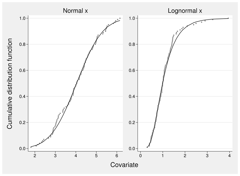
The acd transformation smoothly maps the observed distribution of a continuous covariate onto one scale, namely, that of an approximate uniform distribution on the interval (0, 1). If the relationship between a response Y and acd (X) is linear, say, E (Y) = β₀ + β₁acd (X), the relationship between Y and X is nonlinear and is typically sigmoid in shape (see, for example, figure 1 in the next section). The parameters β₀ and β₀ + β₁ in such a model are interpreted as the expected values of Y at the minimum and maximum of X, that is, at acd (X) = 0 and 1, respectively. The parameter β₁ represents the range of predictions of E(Y) across the whole observed distribution of X.

Figure 1.

ecdf and acd values for samples from a normal and a lognormal distribution, n = 100. Solid line: fitted acd curve; dots, ecdf.

2.3. Example 1: Simulated distributions

Figure 1 shows the ecdf and acd values for a normal distribution, X ~ N (4, 1), and a lognormal distribution, ln (X) ~ N (0, 0.5²), in simulated samples of size n = 100. The positive skewness of the lognormal sample is apparent from the asymmetric shape of the ecdf curve. The upper-tail region of the lognormal distribution is compressed by the acd transformation, and the lower-tail region is much less compressed.

2.4. Example 2: Kidney cancer data

RE04 is a large randomized, controlled trial in metastatic kidney cancer conducted by the uk Medical Research Council (Gore et al. 2010). Patients were randomized 1:1 to standard immunotherapy (interferon-α) or triple therapy (interferon-α, interleukin-2, 5-fluorouracil). The primary outcome measure was time to death from any cause (that is, overall survival). Of the 1,006 patients recruited to the trial, 691 died during the follow-up phase. Triple therapy did not improve survival compared with standard immunotherapy (hazard ratio = 1.05, 95% confidence interval (ci) [0.90, 1.21]).

Several standard prognostic factors for the clinical course of the disease were measured at randomization. These included hemoglobin (haem), of which low values (suggesting anemia) tend to predict shorter survival times. The dataset that we analyze (re04_haem.dta) contains the 999 patients with follow-up at the time of analysis and is limited to the survival data and haem. As an example of acd analysis, we investigate the functional form of the effect of haem on the log relative-hazard in univariate Cox models. Because haem is only weakly correlated with other prognostic factors, we would expect little confounding when ignoring the other factors.

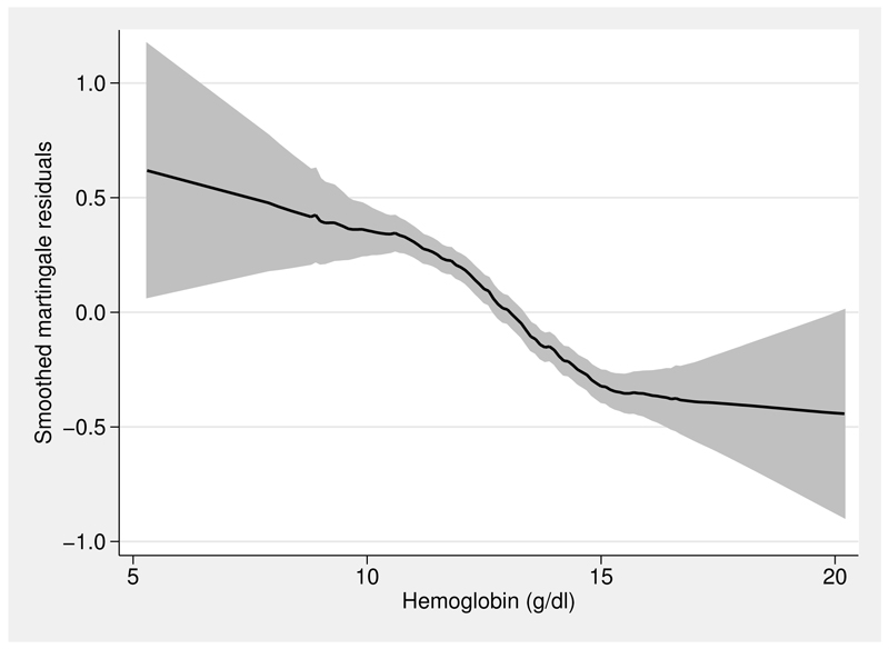
Figure 2 provides a rough guide to the shape of the functional form needed for haem. A running-line smoother (Sasieni, Royston, and Cox 2005) on haem of the martingale residuals from a null Cox model is shown. The plot was created as follows:

Figure 2.

Running-line smoother fit to the martingale residuals from a null Cox model for the re04 trial data

• stcox, estimate

• predict mg, mgale

• running mg haem, nopts span(0.5)

Because martingale residuals are generally “noisy”, the option span(0.5) was specified to increase the smoothness of the fitted line compared with the default span (for these data, of 0.25).

The functional form appears distinctively sigmoid. Most of the prognostic effect of haem occurs between about 10 and 15 g/dl, which are the 5th and 86th centiles of the sample of haem values.

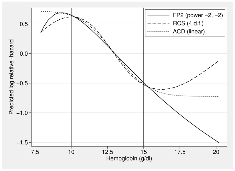
We now investigate the functional form according to recognized tools used with Cox and many other regression models: fps (fracpoly, or in Stata 13, the fp command) and rcs (the uvrs command) (Royston and Sauerbrei 2007). Figure 3 shows the estimated log relative-hazard, centered on the mean haem value of 13.0 g/dl, for the best-fitting two-term fp (fp2) curve and for an rcs with 4 degrees of freedom (d.f.) (3 interior knots).

Figure 3.

The fitted values (log relative-hazard) for three functions of haem. Vertical lines delineate a region with the highest data density. See text for details.

The three functions were all estimated by Cox regression models. They agree closely in the region between 10 and 15 g/dl, where the data density is highest. They differ substantially at more extreme values of hemoglobin, where only the acd approach gives a sigmoid curve that agrees qualitatively with the picture in figure 2. The Akaike information criterion values (−2 × log partial likelihood + 2 × model dimension) for the three models are 8,508.3 (fp2), 8,502.08 (rcs) and 8,497.8 (linear function of acd-transformed haem). On this measure, the acd-based model is preferred.

If the functional form is simplified by removing terms that are statistically insignificant at the 5% level, the fp2 function is replaced by a straight line, and the spline function is replaced by another line of similar shape to that in figure 3 but with one fewer knot. The deviance (−2 × log partial likelihood) of the acd function is 9.5 lower than that of the linear function. Nonnested model analysis shows that the acd function fits significantly better (P < 0.001) than a straight line.

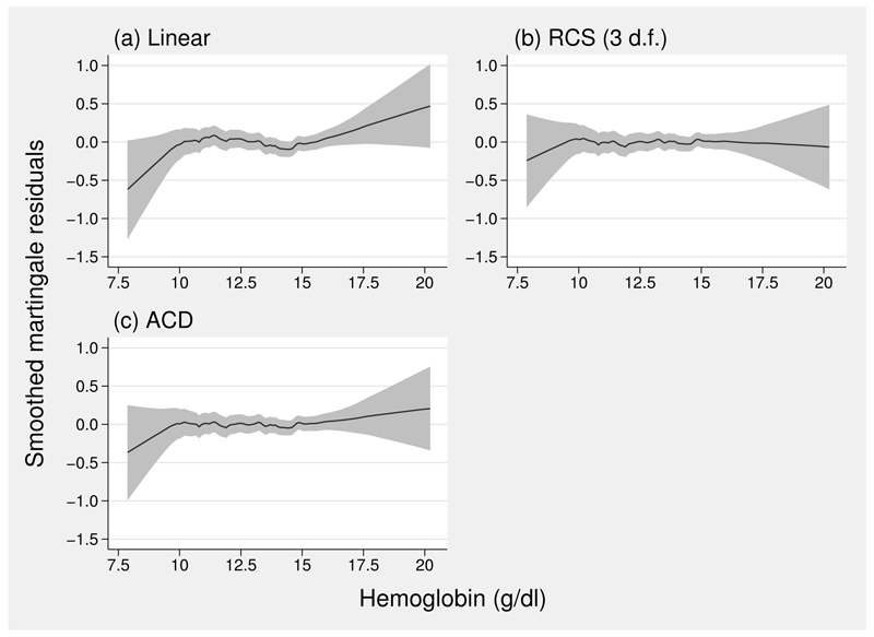
For the acd transformation, the best-fitting power p in (1) is 1, and the corresponding parameters β₀ and β₁ are estimated to be −6.98 and 0.536, respectively. In this example, no fp transformation of the resulting a_i is needed to provide a good fit in the Cox regression model, but this is not always the case. Figure 4 shows smoothed martingale residuals from Cox models with linear, reduced rcs (3 d.f.), and acd models for haem. The linear function is a poor fit. The other two fits are good, but as we noted in figure 3, the spline function is not sigmoid, which on substantive grounds may be unsatisfactory here.

Figure 4.

Smoothed martingale residuals from three Cox models for the covariate haem. (a) Linear; (b) rcs with 3 d.f.; (c) linear function of acd(haem).

In the Cox regression on acd(haem), the estimated regression coefficient is −1.44 (95% ci [−1.70, −1.18]). Thus the model-based estimate of the hazard ratio between the minimum and maximum values of haem is 0.24 (ci [0.18, 0.31]). That represents about a fourfold range.

2.5. Example 3: Melanoma thickness

The next example is more challenging than the others. Cutaneous malignant melanoma is a type of skin cancer that is most prevalent in sunny countries with a substantial proportion of fair-skinned people, such as Australia. The depth of invasion of the tumor is the dominant prognostic factor determining the long-term survival chances of the patient.

We consider a large dataset (n = 28656) of melanoma patients from the Queensland Cancer Registry in northeastern Australia. Cancer-specific survival time and (among several other known prognostic variables) tumor thickness (thick) in mm were recorded in patients diagnosed from 1995 to 2008 (Baade et al. 2013). The 10-year cancer-specific survival probability was 92.6%. For reasons of confidentiality, 5% of the observations we analyze here have been slightly perturbed at random.

We analyze the univariate relationship between tumor thickness and survival. Following preliminary investigation of the appropriate scaling for covariate effects, we chose a class of flexible parametric models (Royston and Lambert 2011) with a probit link. The models are implemented through the scale(normal) option of the stpm2 command (Lambert and Royston 2009).

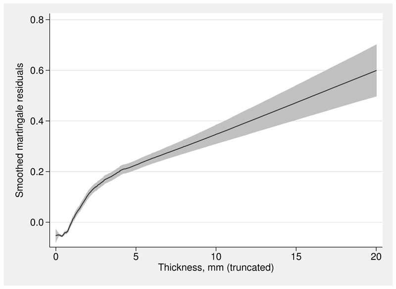
Logically, because a thicker tumor is more dangerous, we expect the relationship between thickness and mortality to be monotone increasing. To ensure monotonicity, we start by restricting ourselves to one-term fp (fp1) models for thickness. Figure 5 shows a running-line smooth of the relationship between thick and the martingale residuals from the null flexible parametric model with probit link. Because the distribution of thick is a highly positively skew (coefficient of skewness = 8.5), we truncate thick at 20 mm (the 99.92 percentile) for better visualization of the lower values.

Figure 5.

Smoothed martingale residuals for a null flexible parametric model on truncated tumor thickness

The functional form appears to be something like a straight line superimposed on a doubly asymptotic curve. Clearly, no simple fp model can represent it accurately. Instead, we construct an fp model comprising thick and its acd transformation, athick. These variables are highly correlated. To reduce overfitting and instability, we allow at most fp1 transformations. The two variables thick and athick need to be modeled simultaneously. For this purpose, we apply the mfp command for multivariable fp modeling to the variables, restricting each predictor to fp1 through the dfdefault(2) option of mfp:

• use melanoma

• (Queensland melanoma data (5%, random perturbation))

• acd athick=thick

• mfp, dfdefault(2): stpm2 thick athick, df(3) scale(normal)

• Deviance for model with all terms untransformed = 12153.785, 28027 observations

• (output omitted)

• Final multivariable fractional polynomial model for _t

Variable	——Initial——			——Final——
	df	Select	Alpha	Status	df	Powers
thickness	2	1.0000	0.0500	in	1	1
athick	2	1.0000	0.0500	in	2	3

Log likelihood = -6001.0779           Number of obs =   28027

	Coef.	Std. Err.	z	P>|z|	[95% Conf. Interval]
xb
Ithic__1	.0383586	.0060483	6.34	0.000	.0265042	.050213
Iathi__1	2.174268	.0600696	36.20	0.000	2.056534	2.292003
_rcs1	.3733268	.0078263	47.70	0.000	.3579876	.3886661
_rcs2	.0567674	.0070334	8.07	0.000	.0429823	.0705525
_rcs3	.0403051	.0051965	7.76	0.000	.0301202	.0504901
_cons	-2.279906	.0235895	-96.65	0.000	-2.326141	-2.233671

Deviance:12002.156.

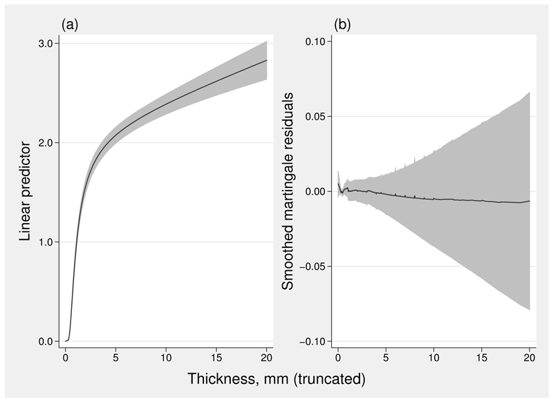
The selected model is linear in thick (variable Ithic__1, created by mfp) and fp1 with power 3 in athick (variable Iathi__1, also created by mfp). The resulting linear predictor quantifies the difference in the probit of the cumulative probability of dying from melanoma up to any given time point. The linear predictor and the smoothed martingale residuals are shown in figure 6. In figure 6(a), a linear predictor value of 0 corresponds to patients with the smallest tumors and hence the lowest mortality.

Figure 6.

(a) Linear predictor from flexible parametric model; (b) smoothed martingale residuals from the same model. Shaded areas represent 95% pointwise cis. Tumor thickness has been truncated at 20 mm.

The shape of the fitted linear predictor resembles that of the null-model martingale residuals in figure 5. Because the two estimated curves are on different scales, they are not numerically comparable. As shown in figure 6(b), the martingale residuals from the model comprising thick and acd(thick)³ show no discernible pattern or trend, which suggests that we have an excellent fit to the data.

2.6. Example 4: Approximating an unusual functional form

Primary biliary cirrhosis (pbc) is a serious liver disease that usually results in liver failure and death. A particular pbc dataset has been reanalyzed several times in the literature to illustrate aspects of survival analysis. We use data on 312 patients (125 deaths from any cause, 187 censored observations) obtained in a randomized controlled trial of two treatments for pbc that was performed at the Mayo Clinic between 1974 and 1984.

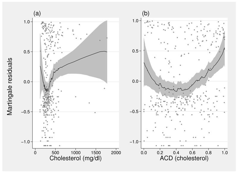
Several potentially prognostic variables were measured at baseline. Figure 7(a) shows raw and smoothed martingale residuals from a null Cox model for one of the variables, chol (serum cholesterol, mg/dl). The trench-shaped functional form shown in figure 7(a) is rather unusual and is not easy to model convincingly, for example, using fps. Figure 7(b) shows the same relation, except the residuals have been smoothed on the acd transformation of chol instead of on the untransformed chol. The shape is now roughly quadratic and is much easier to model using fps (results not shown).

Figure 7.

Raw and smoothed martingale residuals for chol in the pbc dataset: (a) on the original scale of chol; (b) on acd-transformed chol.

3. The acd command

3.1. Syntax

The syntax of acd is as follows:

acd newvar = exp [if] [in] [, all b (#1 #2) power(#) shift(#) ]

3.2. Description

acd transforms a variable or expression exp to newvar, a smooth approximation to its cumulative distribution function. Such transformed covariates may be useful in representing sigmoid relationships in regression models.

3.3. Options

all computes the acd transformation over all available observations by using parameter estimates derived only from observations in the if and in qualifiers.

b(#1 #2) specifies #1 to be the intercept (β₀) and #2 to be the slope (β₁) in the model $\widehat{z}={\beta }_0+{\beta }_1\times {(exp+\text{shift})}^p$. #1 and #2 are both required. If b() is not specified (default case), #1 and #2 are determined from the data by fracpoly.

power(#) specifies p = # in the regression of the transformed ranks, z, on (exp + shift)^p. By default, p is determined automatically by fracpoly from the data. If power() is specified, then shift() must also be specified. A linear function is specified by power(1) and a logarithmic function by power(0).

shift(#) specifies shift = # in the regression of the transformed ranks, z, on (exp + shift)^p. By default, shift is determined automatically by fracpoly from the data. If shift() is specified, then power() must also be specified. The default is shift(0).

4. Conclusion

The acd program may provide a solution to the need for flexible parametric modeling of a covariate effect whose functional form is singly or doubly asymptotic or which has a sigmoid shape or component, as in the melanoma and pbc examples. We have illustrated its use mainly in models with one predictor, but it is also appropriate to use within multivariable modeling. More generally, the acd transformation may play a role in improving the accuracy of predictions from models that include covariates with a markedly skew distribution.

About the author

Patrick Royston is a medical statistician with more than 30 years of experience, with a strong interest in biostatistical methods and in statistical computing and algorithms. He works largely in methodological issues in the design and analysis of clinical trials and observational studies. He is currently focusing on alternative outcome measures in trials with a time-to-event outcome; on problems of model building and validation with survival data, including prognostic factor studies and treatment-covariate interactions; on parametric modeling of survival data; and on novel clinical trial designs.