Automated Digital Dental Articulation

Abstract

Articulating digital dental models is often inaccurate and very time-consuming. This paper presents an automated approach to efficiently articulate digital dental models to maximum intercuspation (MI). There are two steps in our method. The first step is to position the models to an initial position based on dental curves and a point matching algorithm. The second step is to finally position the models to the MI position based on our novel approach of using iterative surface-based minimum distance mapping with collision constraints. Finally, our method was validated using 12 sets of digital dental models. The results showed that using our method the digital dental models can be accurately and effectively articulated to MI position.

1 Introduction

With the giant leap of computer technology, more and more dental offices are going to digital and replacing their traditional stone dental casts with digital dental models. The digital dental models are the exact replica of the teeth. They are usually generated by scanning dental impressions or stone dental models, or directly scanning the teeth intraorally. By incorporating the digital dental models into a 3D head model [1, 2], the orthodontic and orthognathic treatment can be entirely planned within a computer, and thus significantly improve the treatment outcome and decrease the planning time [3]. However, the utilization of digital dental models also creates a new problem in which the reestablishment of the dental occlusion to a maximum intercuspation (MI) position has become more difficult and time consuming than before. A main goal of the orthodontic and orthognathic treatment is to reestablish patient’s occlusion. When doctors use plaster dental models to establish the occlusion, the physical action of aligning upper and lower dental models into MI position is quick and accurate, usually in a matter of seconds. The same is not true in the virtual world, where the dental arches are represented by two 3D images that lack collision constraints. The computer system does not stop the images from moving through each other once the models have made contact. In addition, the operator has no tactile feedback when articulating the digital models. Virtual articulation of an arch of 14 upper teeth against 14 lower teeth into their best possible intercuspation is a complex task. Ideally, the 14 buccal cusps and 4 incisal edges of the mandibular teeth will make maximal contact against the corresponding fossae, marginal ridges and lingual surfaces of the maxillary teeth at MI position. At the same time, the palatal cusps of the maxillary teeth also need to make contact against the fossae and marginal ridges of the lower teeth. Moreover, the dental midlines should be coincidental, and the transverse relationship between the teeth should be appropriate. Finally, all of this needs to be accomplished without creating unwanted areas of overlap. Because of these difficulties, it usually takes close to an hour to achieve the “visually best possible” intercuspation in the computer. More importantly, it is almost impossible to be certain that what is seen in the computer represents the true best possible alignment. Therefore, there is an urgent need to develop a method that is capable of efficiently articulating the upper and lower digital dental models to MI position.

To this end, the purpose of this study is to develop an effective approach to automatically articulate the digital dental models. Our approach includes two steps. The first step is to position the models to an initial position based on dental curves and point matching algorithm. The second step is to finally position the models to the MI position based on iterative surface-based minimum distance mapping (ISMDM) algorithm with collision constraints. Finally, our method was validated using 12 sets of digital dental models.

2 Algorithm Development

2.1 Data Acquisition and Preparation

Three sets of stone dental cases were randomly selected from our dental model archive. An experienced doctor first hand articulated each set of the stone casts to MI position. They were then mounted on a specially designed mounting jig to keep their MI relationship. The mounted models were finally scanned using a 3D laser scanner (0.1mm of scanning accuracy) by a commercially available service (GeoDigm Corp, Chanhassen, MN). This resulted in a set of digital dental models at MI position and saved in stereolithography (.STL) format. Because of the triangulated surface of the model, the upper and lower digital models were slightly outwards expanded and penetrated to each other with a range of 0.08–0.20 mm at MI position, which did not exist in their physical form (stone casts). These scanned models served as a gold standard. Prior to the algorithm development, the lower models were disarticulated in 3D by randomly rotational and translational transformations.

2.2 Initial Alignment

The main purpose of initial alignment is to obtain approximate dental occlusion before two dental models are finally articulated to an accurate and collision-free position and orientation. When the two dental models are initially disarticulated and located at an arbitrary orientation and position in a Cartesian coordinate system, it is necessary to estimate a transformation to bring them relatively close to each other. Two pairs of corresponding curves are extracted and matched from the upper and lower dental models. The first pair is the buccal cusps of the lower arch (Fig. 1b) corresponding to the central groove of the upper arch (Fig. 1a), while the second pair is the palatal cusps of the upper arch corresponding to the central groove of the lower arch. These curves can be viewed as 3D continuous curves (not necessarily fitting polynomial curves) along the dental arches. In this article we only use the first pair as an example.

Fig. 1.

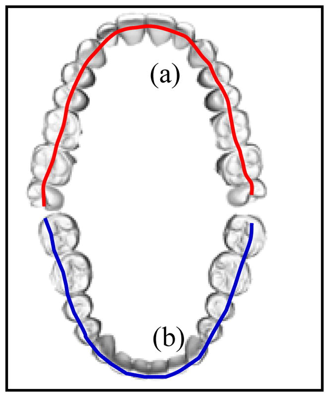
Upper (a) and lower (b) dental curves

Based on the above assumptions, we developed an automated approach to initially position the models. In the first step, we identify the feature points on cusps, incisal edges, central grooves, pits, and fossae to approximately represent the dental curves along the arches. In the second step, the dental curves of the upper and lower arches are matched using a point matching algorithm to complete the initial alignment.

Step 1: Identification of Feature Points on Upper and Lower Occlusal Surfaces

A 2D range image (the heights of the digital model in the z - coordinate) is first calculated for lower arch. Based on the range image and the two-step curve fitting approach [4], we can then compute a 2D fourth-order polynomial dental fitting curve that fits buccal cusps and incisal edges of lower arch in least square. Finally, with the aid of 2D fitting curves, the 3D feature points of the lower occlusal surface can be extracted by detecting the peaks along the lower fitting curve. Similarly, the 3D feature points of upper occlusal surfaces can be identified by detecting the central groove along the upper fitting curve.

Step 2: Point Matching Algorithm

Let ${\{{\mathit{p}}_i\}}_{i=0}^{N-1}$ and ${\{{\mathit{q}}_j\}}_{j=0}^{K-1}$ be sets of 3D feature points of the upper and lower dental models obtained in Step 1. The two sets of points are matched by applying our point matching approach as if the dental curves fit together when dental models are in the MI. Our point matching algorithm (an improved iterative closest points algorithm [5]) is based on graduated assignment combining “softassign” method [6] and a weighted least squares optimization [7]. The initial alignment becomes to find a transformation (R,t) and a correspondence between two sets of feature points {p_i} and{q_j}, and to minimize an energy function in the standard point matching algorithm [6].

2.3 Final Alignment

After the dental models are aligned to an approximate occlusion, they can be finally digitally articulated using our algorithm, Iterative Surface-based Minimum Distance Mapping (ISMDM). The criterion based on maximal contact of the teeth at MI is the key to develop the ISMDM. The dental model articulation can be modeled by consecutive executions of translations and rotations with continuous changes of rotational origin on the lower dental model. In order to automatically achieve maximal contact between upper and lower teeth and reach the MI position, we model this movement by iteratively minimizing distance of surfaces between lower and upper teeth. This method is based on the idea of the iterative closest point algorithm [8] that is generally used in shape matching, registration, and alignment of two similar datasets from the same object. In addition, an important component in our ISMDM method is that we add constraints to prevent the two surfaces from overlap [9]. The detailed computational algorithms are described as follows.

The Modelling of Dental Occlusion

Let ${\{{\mathit{u}}_i\}}_{i=0}^{M-1}$ and ${\{{\mathit{v}}_j\}}_{j=0}^{J-1}$ be 2 sets of M and J vertices in the meshes of the digital upper and lower dental models, respectively. In the following, we assume the upper model is in a static position. The transformations and rotations are only performed on the lower dental model. The transformed v_j is modeled as:

$${\mathit{v}}_j^{\prime }(\stackrel{\sim }{\mathit{R}},\stackrel{\sim }{\mathit{t}})\equiv \stackrel{\sim }{\mathit{R}}({\mathit{v}}_j-\stackrel{\sim }{\mathit{o}})+\stackrel{\sim }{\mathit{o}}+\stackrel{\sim }{\mathit{t}}$$ (1)

where õ is a rotational origin (the pivot point) of the rotation matrix R̃, and t̃ is the translation vector. Maximizing contact area is equivalent to maximizing the number of contacting vertices in {v_j}. However, not every vertex in {v_j} will make contact when the models are in the MI. Those contact areas are even more difficult to be predicted precisely. Therefore, we model the distance of surfaces between lower and upper teeth as:

$$d_S\equiv \sqrt{\frac{1}{J}\sum _{j=0}^{J-1}{\Vert {\mathit{u}}_{i_j}-{\mathit{v}}_j\Vert }^2}.$$ (2)

u_ij is a point closest to v_j and given by:

$${\mathit{u}}_{i_j}=\mathit{arg}\underset{\mathit{u}\in \{{\mathit{u}}_i\}}{\mathit{min}}\Vert \mathit{u}-{\mathit{v}}_j\Vert$$ (3)

where i_j∈{0,1,⋯ M−1}. Instead of directly maximizing contact area, we increase the chances of making contact by minimizing d_S.

Because the 2 digital models should not penetrate to each other, adding collision constraints is the most important step in digital dental occlusion. The avoidance of collision is formulated as constraints and will be incorporated into the optimization programming. Let 𝓟_j be a plane with a unit normal vector n_j and a point r_j on it. When the transformed vertex ${\mathit{v}}_j^{\prime }(\stackrel{\sim }{\mathit{R}},\stackrel{\sim }{\mathit{t}})$ is not allowed to be at the opposite side of the plane 𝓟_j, the constraint can be expressed as

$${\left({\mathit{v}}_j^{\prime }(\stackrel{\sim }{\mathit{R}},\stackrel{\sim }{\mathit{t}})-{\mathit{r}}_j\right)}^T{\mathit{n}}_j>0.$$ (4)

r_j can be given by

$${\mathit{r}}_j-{\mathit{u}}_{i_j}-\delta {\mathit{n}}_j$$ (5)

where δ is allowable penetration depth (0.1mm of tolerance to compensate outwards expansion of triangulated surface) for the lower teeth. The unit normal vector n_j can be chosen by calculating the average normal at the vertex u_ij. Since some areas between upper and lower teeth will never make contact during the MI, a large number of constraints added to the algorithm may be redundant. In order to reduce the number of constraints, it is not necessary to add a constraint to a point pair v_j and u_ij if the distance between them is beyond a threshold ρ.

Minimization of the Distance of Occlusal Surfaces and the Algorithm

Given a rotational origin õ, we calculate the rotation matrix R̃ and the translation vector t̃ which minimize

$${d_S}^2(\stackrel{\sim }{\mathit{R}},\stackrel{\sim }{\mathit{t}})\equiv \sum _{j=0}^{J-1}{\Vert {\mathit{u}}_{i_j}-{\mathit{v}}_j^{\prime }(\stackrel{\sim }{\mathit{R}},\stackrel{\sim }{\mathit{t}})\Vert }^2,\text{subject}\text{to}{\left({\mathit{v}}_j^{\prime }(\stackrel{\sim }{\mathit{R}},\stackrel{\sim }{\mathit{t}})-{\mathit{r}}_j\right)}^T{\mathit{n}}_j>0$$ (6)

The rotation matrix consists of non-linear terms which can be linearized by small-angle approximation [10, 11]. When the 2 dental models are getting occluded, the increment needed to seat the lower model will gradually become smaller. Therefore, errors caused by this approximation will become less significant. Approximate the rotational matrix R̃ by linearizing it as

$$\stackrel{\sim }{\mathit{R}}=\left(\begin{array}{ccc}1& -{\theta }_z& -{\theta }_y\\ {\theta }_z& 1& -{\theta }_x\\ {\theta }_y& {\theta }_x& 1\end{array}\right)$$ (7)

where θ_x, θ_y, and θ_z are rotational angles with respect to x–, y–, and z– axes. Define θ=(θ_x, θ_y, θ_z)^T and L_j as:

$${\mathit{L}}_j\equiv \left(\begin{array}{ccc}0& -v_{j,z}+{\stackrel{\sim }{o}}_z& -v_{j,y}+{\stackrel{\sim }{o}}_y\\ -v_{j,z}+{\stackrel{\sim }{o}}_z& 0& v_{j,x}-{\stackrel{\sim }{o}}_x\\ v_{j,y}-{\stackrel{\sim }{o}}_y& v_{j,x}-{\stackrel{\sim }{o}}_x& 0\end{array}\right).$$ (8)

(R̃−I)(v_j−õ) can be rewritten as: (R̃−I)(v_j−õ) = L_jθ. Let b_j = v_j−u_ij, x ≡ (t̃^T,θ)^T = (t̃_x, t̃_y, t̃_z, θ_x, θ_y, θ_z)^T, and ${\stackrel{\sim }{\mathit{L}}}_j\equiv \left[\begin{array}{cc}{\mathit{L}}_j& \mathit{I}\end{array}\right]$. The objective function in Equation (6) becomes:

$${d_S}^2(\stackrel{\sim }{\mathit{R}},\stackrel{\sim }{\mathit{t}})={\mathit{x}}^T\left(\sum _{j=0}^{J-1}{{\stackrel{\sim }{\mathit{L}}}_j}^T{\stackrel{\sim }{\mathit{L}}}_j\right)\mathit{x}+2\left(\sum _{j=0}^{J-1}{{\mathit{b}}_j}^T{\stackrel{\sim }{\mathit{L}}}_j\right)\mathit{x}+\sum _{j=0}^{J-1}{\Vert {\mathit{b}}_j\Vert }^2.$$ (9)

With the linearization of rotation matrix, the objective function d_S²(R̃, t̃) becomes a quadratic form, and (4) becomes a linear constraint. The minimization of (6) can be solved by quadratic programming.

3 Validations and Results

Twelve sets of the stone dental casts were used to validate our approach. They were randomly selected from our dental model archive. The models used for algorithm development were excluded. The selection criteria included no early contact and a stable occlusion. All the models had relatively normal and full dentition except 4 pairs were partial edentulous. The models were scanned at MI position using the method described in 2.1. These digital dental models at MI position served as a control group.

The models were positioned in Cartesian coordinate system. The origin O was the centroid of the boundary box of the lower model (Fig 2). Three landmarks commonly used in clinic were digitized. They were mesiobuccal cusps of the first right and left molars (A and B), and central dental midline (C). The coordinates of each landmark were used later to compare with the same landmarks in the experimental group.

Fig. 2.

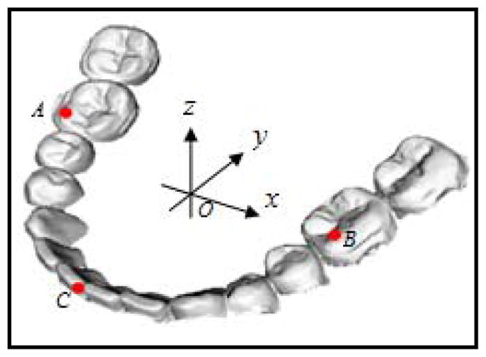
Coordinate system

In order to establish an experimental group, lower models and their landmarks were duplicated. Because the models were scanned at MI position, it was necessary to disarticulate the duplicated lower model from its original position. The lower model was first randomly rotated around the X-, Y-, Z- axes angles between $\left[-\frac{1}{3}\pi ,\frac{1}{3}\pi \right]$, respectively. It was then randomly translated in millimeters between [−20,20] along the X-, Y-, and Z- axes, respectively. During the rotational and translational transformations, the landmarks were “glued” on the lower model and transformed with it. We believed that these transformations were randomly enough to disarticulate the lower models from their MI position. These disarticulated lower models served as an experimental group. The centroid O, the x-, y- and z- coordinates, and the landmarks A, B and C in the control model became centroid O′, the x′–, y′– and z′ – coordinates, and the landmarks A′, B′ and C′ in the experimental model.

In the experimental group, the upper and lower models were first articulated using our initial alignment algorithm, followed by our ISMDM algorithm with the following parameters: S = 60 (iterations of ISMDM), ρ = 0.2 mm and δ = 0.1 mm. Fig. 3 showed a plot of average distance of surface d_S versus iteration k for all 12 sets of the models using the ISMDM algorithm. During the articulation process, the upper model remained static while the lower model sought its MI position. In the initial alignment, the point match algorithm is applied only to the feature points of the models. This may cause collisions between the lower and upper teeth. After they are fed into the ISMDM, the collision constrain will force the lower model out of the upper model until the models are free of collision. This is why the average distance ds between surfaces of lower and upper models is smaller at the beginning than it is at the final position after 60 iterations. The entire process was completed using a regular office PC computer with an Intel P4 2.2GHz CPU and 4GB memories.

Fig. 3.

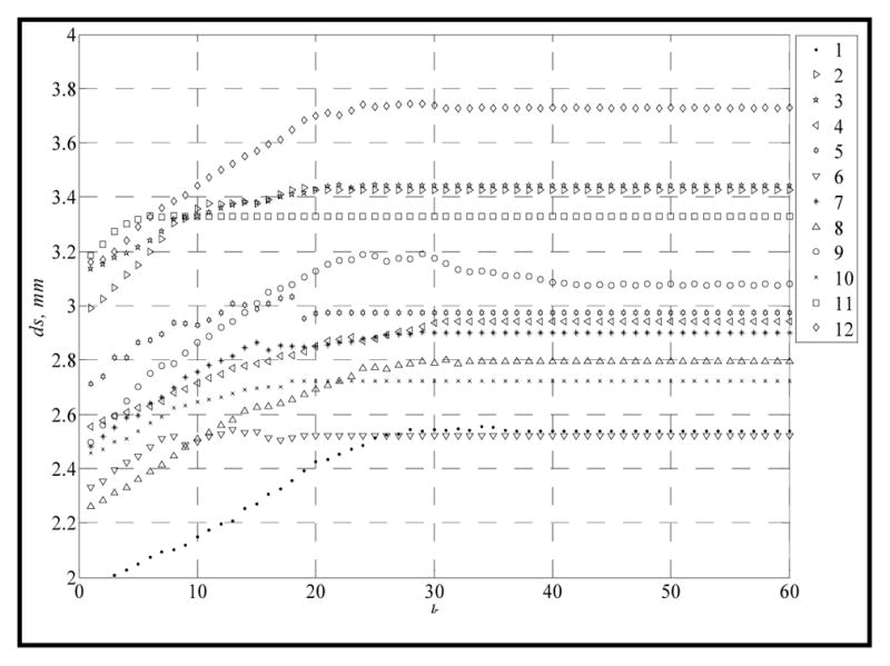
Articulation results using ISMDM algorithm.

Finally, the validation was completed by calculating the transitional and rotational deviations of the lower models between the experimental and control groups. Based on our clinical experience, there would be no clinical significance if the translational deviation of the lower dental models between the control the experimental groups is less than 0.5mm in each X, Y and Z direction and the angular deviation is less than 1° on sagittal, coronal, and axial planes, respectively.

Translational Deviations between the Experimental and Control Groups

The means and standard deviations (SD) of the translational differences between the experimental and control models were computed. The mesiobuccal cusp of the first right molar(A′,A) and the first left molar(B′,B), the central dental midline(C′,C), and the centroid(O′,O) were computed in x–, y–, and z– axis, respectively (Table 1). It indicated that the models were articulated successfully with a small degree of translational deviation with no clinical significance.

Table 1.

Translational Deviations (mean ± SD, calculated in mm)

	Initial alignment			Final alignment (ISMDM)
	x	y	z	x	y	z
(A′, A)	−0.0938 ± 0.5873	0.4451 ± 1.2834	1.6366 ± 0.6841	−0.0661 ± 0.3828	−0.1206 ± 0.5621	0.1318 ± 0.2185
(B′, B)	−0.1471 ± 0.5935	0.5708 ± 1.0660	1.6332 ± 0.5336	−0.0697 ± 0.3794	−0.1793 ± 0.4606	0.1707 ± 0.1151
(C′, C)	−0.0596 ± 0.7824	0.5433 ± 0.7382	0.5394 ± 0.6998	−0.1088 ± 0.3380	−0.1449 ± 0.2059	0.1214 ± 0.2830
(O′, O)	−0.0917 ± 0.4310	0.5912 ± 0.6965	1.3714 ± 0.4399	−0.0735 ± 0.2926	−0.1481 ± 0.1829	0.1464 ± 0.1026

Angular Deviations between the Experimental and Control Groups

The angular differences between the experimental and control models were computed on sagittal (Y-O-Z), coronal (X-O-Z), and axial (X-O-Y) planes, respectively. In order to computer the angular deviation, the models in experimental group were moved translationally so that the centroid O′ was matched to the centroid O in the control group. Afterwards, z′– axis was projected onto the Y-O-Z plane. The sagittal angular deviation ω̂_x was defined by the angle between the projected z′– axis and z– axis on the Y-O-Z plane. By the same token, by projecting the z′– axis onto the X-O-Z plane, the coronal angular deviation ω̂_y was defined by the angle between the projected z′– and z– axis on the X-O-Z plane. Furthermore, by projecting the y′– axis onto the X-O-Y plane, the axial angular deviation ω̂_z was defined by the angle between the projected y′– axis and y– axis on the X-O-Y plane. Finally, the means and SDs of the angular deviations between the experimental and control models were computed (Table 2). It indicated that the models are successfully articulated with only a small degree of rotational deviation that had no clinical significance.

Table 2.

Angular Deviations

	Initial alignment	Final alignment
ω̂x	−2.3016 ± 2.0818	−0.0850 ± 0.7459
ω̂y	0.0102 ± 0.4752	−0.0624 ± 0.2322
ω̂z	−0.1507 ± 2.2328	0.0717 ± 1.1453

4 Discussion

We have developed an automated approach to digitally articulate dental models. This approach consists of two major steps. The first step is the initial alignment, which using the point match algorithm to match the feature points of dental curves in order to bring the models relatively close to each other. The second step is the final alignment, which uses the ISMDM algorithm to minimize the average distance of surfaces of the models in order to articulate the upper and lower models to the MI without overlapping. This approach has been validated using 12 sets of the dental models. The results showed the models were successfully articulated with a small degree of deviation that did not have clinical significance.

Our approach is robust. First, the initial alignment algorithm itself can bring the models to a closed position to the final occlusion. This can significantly reduce the number of executions of nearest point searching of ISMDM. Second, each lower model can be effectively docked to a final occlusion after the average distance of surface d_S converges at k < 30 using our ISMDM algorithm. The deviations are small enough to meet clinical standard. Third, our ISMDM algorithm has successfully overcome the notorious uncontrollable overlapping problem between the upper and the lower models. This is done by applying linear constraints and allowable tolerance of penetration depth δ. In this experiment, we set the penetration depth was 0.1mm. Fourth, as indicated in validation, our ISMDM algorithm can also be used to articulate the partially edentulous models.

Finally, our approach is different from others. Hiew et al. [9] used the right and posterior surfaces of the model bases, rather than based on the occlusal criteria, to perform the dental model alignment. Zhang et al. [12] designed a two-stage occlusal analysis algorithm to manually alignment the models in the computer. Finally, DeLong et al. [13] utilized a “3-point alignment” method by first identifying 3 pairs of contacting points on both the upper and lower stone models, digitizing them onto the digital models, and finally matching the corresponding points using a fitting algorithm to bring the digital models together. The results were visually checked and process was repeated until the visual outcome was satisfactory. We found it is almost impossible to be certain that what is seen in the computer truly represents the best possible alignment. Comparing to the above methods, our method is practical and can be immediately used in the patient treatment planning process.

References

- 1.Gateno J, Xia JJ, Teichgraeber JF, Christensen AM, Lemoine JJ, Liebschner MA, Gliddon MJ, Briggs ME. Clinical feasibility of computer-aided surgical simulation (CASS) in the treatment of complex cranio-maxillofacial deformities. J Oral Maxillofac Surg. 2007 Apr;65:728–34. doi: 10.1016/j.joms.2006.04.001. [DOI] [PubMed] [Google Scholar]
- 2.Xia JJ, Gateno J, Teichgraeber JF. New Clinical Protocol to Evaluate Craniomaxillofacial Deformity and Plan Surgical Correction. Journal of Oral and Maxillofacial Surgery. 2009;67:2093–2106. doi: 10.1016/j.joms.2009.04.057. [DOI] [PMC free article] [PubMed] [Google Scholar]
- 3.Xia JJ, Gateno J, Teichgraeber JF, Christensen AM, Lasky RE, Lemoine JJ, Liebschner MA. Accuracy of the computer-aided surgical simulation (CASS) system in the treatment of patients with complex craniomaxillofacial deformity: A pilot study. J Oral Maxillofac Surg. 2007 Feb;65:248–54. doi: 10.1016/j.joms.2006.10.005. [DOI] [PubMed] [Google Scholar]
- 4.Kondo T, Ong SH, Foong KWC. Tooth segmentation of dental study models using range images. Medical Imaging, IEEE Transactions on. 2004;23:350–362. doi: 10.1109/TMI.2004.824235. [DOI] [PubMed] [Google Scholar]
- 5.Besl PJ, McKay HD. A method for registration of 3-D shapes. IEEE Trans Pattern Analysis and Machine Intelligence. 1992;14:239–256. [Google Scholar]
- 6.Gold S, Rangarajan A, Lu CP, Pappu S, Mjolsness E. New algorithms for 2D and 3D point matching pose estimation and correspondence. Pattern Recognition. 1998;31:1019–1031. [Google Scholar]
- 7.Walker MW, Shao L, Volz RA. Estimating 3-D location parameters using dual number quaternions. CVGIP: Image Understanding. 1991;54:358–367. [Google Scholar]
- 8.Hajnal JV, Hawkes DJ, Hill D. Medical image registration. CRC; 2001. [DOI] [PubMed] [Google Scholar]
- 9.Hiew LT, Ong SH, Foong KWC. Optimal Occlusion Of Teeth. Control, Automation, Robotics and Vision, 2006. ICARCV’06. 9th International Conference on; 2006. pp. 1–5. [Google Scholar]
- 10.Milenkovic VJ, Schmidl H. Optimization-based animation. Proceedings of the 28th annual conference on Computer graphics and interactive techniques; 2001. pp. 37–46. [Google Scholar]
- 11.Zhang L, Kim YJ, Varadhan G, Manocha D. Generalized penetration depth computation. Computer-Aided Design. 2007;39:625–638. [Google Scholar]
- 12.Zhang C, Chen L, Zhang F, Zhang H, Feng H, Dai G. A New Virtual Dynamic Dentomaxillofacial System for Analyzing Mandibular Movement, Occlusal Contact, and TMJ Condition. Lecture Notes in Computer Science. 2007;4561:747. [Google Scholar]
- 13.DeLong R, Ko CC, Anderson GC, Hodges JS, Douglas WH. Comparing maximum intercuspal contacts of virtual dental patients and mounted dental casts. J Prosth Dent. 2002;88:622–630. doi: 10.1067/mpr.2002.129379. [DOI] [PubMed] [Google Scholar]