Small molecular logic systems can draw the outlines of objects via edge visualization

Like a child with a crayon, logical molecules produce outline drawings from a template.

Abstract

The recently-discovered ability of small logical molecules to recognize edges is exploited to achieve outline drawing from binary templates. Outlines of arbitrary curvature, several colours and thicknesses down to 1 mm are drawn in around 30 min or less by employing a common laboratory two-colour ultraviolet lamp. The outlines and the light dose-driven XOR logic with fluorescence output or ‘off–on–off’ action which is observed in the irradiated regions are modelled by combining foundational principles of photochemistry, acid–base neutralization and diffusion.

Introduction

Molecular Boolean logic ^1–8 allows us to achieve information processing tasks in chemical contexts. ‘Off–on’ sensing of atomic species can be seen to be YES logic, whereas related ‘on–off’ sensing is NOT logic. ^9,10 Selective ‘off–on’ sensing of molecular targets, either alone or in groups, is AND logic, ^11–17 since multiple functional groups need to be recognized simultaneously. ‘Off–on–off’ behaviour can visualize windows of species concentration ^18–21 and related XOR logic, following more complex Boolean processing, can perform edge detection.²² Now we show for the first time how small molecular logical systems can achieve outline drawings from templates, rather similar to a portrait artist who sketches a sitter.

Outline drawings form a deep part of our common culture since medieval master artists used outline drawings as cartoons from which the final masterpieces were developed.²³ Outline drawings also form a deep part of our culture as individuals, by accompanying us from the early stages of life. Small children use crayons to draw stick people with large faces. Soon after, their parents bring pictures to be coloured by numbers. These are outline drawings and the children happily overshoot the lines initially during colouring. Quickly, they learn to respect the lines as boundaries between areas. Later they are entertained by outline drawings in cartoons within comic strips²⁴ and video frames. For most of us, outline drawing is unavoidable. This is a human-level computation that we perform consciously, which is now being emulated by designed molecular systems. This is to be contrasted with edge detection itself, which is a human-level computation which occurs while we remain largely unaware of it.

Results and discussion

Imaging

The edge detection experiment²² pivots on a paper prepared by absorbing photoacid generator (triphenylsulfonium chloride) 1,²⁵ one of the H⁺-driven fluorescent ‘off–on’ sensors 2–5 (ref. 26 and 27) and pH buffer Na₂CO₃ in methanol–water (1 : 1, v/v), followed by careful drying at 50 °C for 4 min. The photoacid generator is broken down in irradiated regions to produce protons and a quencher product 6 [2-(phenylthio)biphenyl].²⁵ Even at early exposure times, the proton numbers are sufficient to overcome the local buffer and then bind to the receptor units of the sensor molecules. Being intramolecular, these receptors had efficiently quenched the fluorescence of the sensors until then. Proton binding to these receptors removes this intramolecular quenching and resurrects the fluorescence of the sensors. This creates a positive photograph. However, as the exposure time increases, the quencher product 6 builds up to sufficiently large numbers so that it can interact bimolecularly with the sensor molecules causing their fluorescence to be extinguished again via this new pathway. Thus, the irradiated region displays an ‘off–on–off’ fluorescence response with respect to the radiation dose. At later stages of the experiment, the irradiated regions possess high concentrations of protons and the quencher product 6. The unirradiated regions possess virtually none of these, so that sharp concentration gradients are set up exclusively at the edges between these two regions. Now we get diffusion of these species down these gradients, except that the protons have moved 1–2 mm whereas 6 has hardly moved at all. So the sensor molecules resident in the unirradiated regions adjacent to the boundaries are able to be switched ‘on’ in terms of their fluorescence. The edges alone are lit up in this way.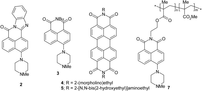

It occurred to us that the processes leading to edge detection can be exploited to achieve outline drawing by logical molecules. It even appears that in portraiture, outline drawings can directly be the visualization of edges of the object which are detected by the artist. The concept behind molecular logic-based outline drawing is summarized in Fig. 1. An object, in the form of a mask, is imaged onto the prepared paper as a positive photograph in a fluorescent colour. This image slightly expands during the course of the experiment due to the proton diffusion process mentioned above. The fluorescence of the original positive photograph is then quenched by the bimolecular process, to leave behind an outline drawing. The prepared paper serves as a graphic user interface, akin to a mouse-driven or touch-sensitive screen of a modern stored-program computer or a canvas in front of the artist. The experiment also requires a two-colour ultraviolet lamp for photochemical writing and reading. This edge detecting system²² is akin to what happens in our eyes ^28,29 or somewhat like what is available within image-handling software running on a stored-program computer.³⁰ Although not claimed as such, excellent (though transient) outline drawing also occurs in a reactive network of relatively high molecular weight oligonucleotides.³¹ The same cannot be said of an edge-detecting bacterial field whose visualized edges are considerable broader.³² We also note that fluorescent positive photographs have been demonstrated by combining 1 and polymeric fluorescent ‘off–on’ sensor 7.³³ More generally, positive photographs represent the object realistically. In contrast, outline drawing involves a degree of abstraction in an artistic sense.

Fig. 1. Drawing the outline of a disc-shaped hole in a mask, by transforming it into a ring image via edge visualization, involves three steps. First, a positive photograph of the disc is imaged in the fluorescent colour of the sensor. Second, the positive photograph is isotropically expanded slightly via a proton diffusion process. Third, the fluorescence of the original positive photograph is erased via a bimolecular quenching process.

Some compounds suitable for the drawing task are already available in our laboratory from other studies. ^26,27 One compound 5 is specifically synthesized by reacting perylenetetracarboxy-dianhydride 8 with N,N-bis(hydroxyethyl)ethylenediamine 9.³⁴

Fig. 2 shows the outline drawings arising from two templates of a shamrock and a bird, which contain lines of varying degrees of curvature. The images are written through the object mask, with 254 nm irradiation. The images are read with 366 nm light after removal of the mask. It is very clear that substantially accurate outline drawings are attained in several colours, simply by varying the fluorescent ‘off–on’ pH sensor. Even the highly curved regions of the feathers of the bird are rendered as outlines of good fidelity.

Fig. 2. Backlit shamrock and bird objects and fluorescence images excited at 366 nm on filter paper with molecular logical mixtures involving pH ‘off–on’ sensors 2, 3, 4 and 5, following writing with 254 nm light for 35, 16, 35 and 35 min respectively (one factor probably contributing to these differing times is the inner filtering of the writing light by the sensor). Preparation of the mixtures and the filter paper are detailed in the experimental section. The filter paper diameter is 11.0 cm in this figure and the next.

The mechanism of outline drawing is investigated by studying a simpler square template, composed exclusively of straight lines and right angles, with the fluorescent ‘off–on’ pH sensor 3, as a function of writing time (Fig. 3). It is gratifying that the experimental results in Fig. 3 largely follow the simple scheme shown in Fig. 1. For quantitation purposes, such as the determination of outline-widths, the images in Fig. 3 are studied with image analysis software to produce intensity–distance profiles (Fig. 4). The intensity, which is plotted in Fig. 4, represents the green channel following a red-green-blue (RGB) colour separation. Whenever the intensity of the green channel saturates, the blue channel data are used instead for the outline-width calculation (see ESI†). The outline-width is calculated similar to that for a full width at half-maximum but with allowance made for the asymmetric effect caused by the two different baseline intensities in the irradiated and unirradiated regions. Brightnesses of the outlines are calculated from the fluorescence intensity ratios between the visualized outline and the backgrounds on either foot (see ESI†). Line-widths of 1–2 mm and brightnesses of 1.2–1.8 are found for the outlines (Tables 1 and 2).

Fig. 3. Backlit square object and fluorescence images excited at 366 nm on filter paper with molecular logical mixture involving pH ‘off–on’ sensor 3, following writing in a single exposure with 254 nm light for the stated times.

Fig. 4. Fluorescence intensity–distance profiles along a horizontal line through the centre of the images arising from the square object and the pH ‘off–on’ sensor 3 (green channel) shown in Fig. 3. For purposes of clarity, all curves are adjusted to coincide at the left-foot of the feature.

Table 1. Full widths of outline drawings in Fig. 3, following analysis in Fig. 4 .

Writing time (min)	Full width (left) (mm)	Full width (right) (mm)
8	1.2	1.1
16	2.1	1.7
32 a	1.9	1.8

^aThe widths are calculated for the 32 min case by analyzing the corresponding intensity – length graph in the blue channel rather than by using the green channel result shown in Fig. 4.

Table 2. Brightnesses of outline drawings in Fig. 3, following analysis in Fig. 4 .

Writing time (min)	Brightness (left)		Brightness (right)
8	1.8	1.2	1.7	1.5
16	1.4	1.2	1.5	1.6

The images in Fig. 3 clearly show that the fluorescence intensity in the centre of the square irradiated region, initially switches ‘on’ and then gradually switches ‘off’. This is light dose-driven fluorescence ‘off–on–off’ or XOR logic behavior, ^35–38 which is caused by two processes which are concerted but whose effects are asynchronous. The initial switching ‘on’ of fluorescence of sensors 2 or 3 occurs by H⁺-induced destabilization of a non-emissive twisted internal charge transfer (TICT) excited state. ^26,39 The corresponding initial switching ‘on’ of fluorescence for systems containing sensors 4 or 5 is due to a H⁺-induced suppression of a photoinduced electron transfer (PET) process. ^27,40–42 These occur as soon as the local Na₂CO₃ buffer is overwhelmed by the photogenerated H⁺, so that the local pH value becomes smaller than the pK _a value of the sensor. The subsequent switching ‘off’ of fluorescence of 2–5 is due to the bimolecular quenching via PET from product 6 as mentioned above. It is worth reiterating that a substantial writing light dose, i.e. a substantial writing time under our illumination conditions, is required to build up 6 to a sufficient local concentration before significant bimolecular quenching of fluorescence can be observed. This light dose-driven fluorescence ‘off–on–off’ behaviour can be modelled rather simply by regarding the process as a titration of the buffer Na₂CO₃ by the photoproduced acid,⁴³ followed by the bimolecular quenching.

Modelling

We develop below a minimal model which can broadly emulate the experimental results.

The photoacid generation by 1 is given by eqn (1).⁴⁴

(H⁺)_total = φIt/V 1

where the proton concentration is (H⁺)_total in a reaction volume V (in L) at time t (in min) when the writing light flux is I (in units of Einstein min^–1). The quantum yield of photoacid generation (φ) is a significant fraction of unity.²⁵Eqn (1) is a simplification, since inner filtering of the writing light by products is neglected.

The carbonate neutralization by acid has been well-studied since classical times, ^43,45,46 and we use the simplest components of these treatments for the present purpose. Carbonate is converted to bicarbonate first by H⁺. The equilibrium constant K _a2 = 4.8 × 10^–11 M and eqn (2) applies to this step.

(H⁺)_free = K _a2·x/(a – x) 2

where the initial carbonate concentration (a = 10^–4 M) falls to the value a – x at time t. The free proton concentration at this point is (H⁺)_free. The value of φIt/V is in the range 0–10^–4 M for this step.

As the acid generation proceeds, bicarbonate is converted to carbonic acid in a separate step. Such a two-step treatment is a simplification but justified by the large difference between K _a2 and K _a1. The equilibrium constant K _a1 = 4.3 × 10^–7 M and eqn (3) applies to this second step.

(H⁺)_free = K _a1·x/(a – x) 3

where the initial bicarbonate concentration (a = 10^–4 M) falls to the value a – x at time t. The value of φIt/V is in the range 10^–4–2 × 10^–4 M but the value of x effective for this second step remains below 10^–4 M. Also, for simplicity, we assume that carbonic acid does not escape in the form of CO₂.

When the second neutralization step is completed, carbonate and bicarbonate have all virtually been replaced by 10^–4 M carbonic acid. So, the Ostwald dilution law⁴⁷ (eqn (4)) applies.

(H⁺)_free = (aK _a1)^1/2 4

where a = 10^–4 M and K _a1 = 4.3 × 10^–7 M. So, (H⁺)_free = 7 × 10^–6 M. So the pH value of the solution at the neutralization point is –log(H⁺)_free = 5.15.

For simplicity, we assume that further photoacid generation adds to this baseline value of (H⁺)_free = 7 × 10^–6 M, until the 10^–3 M 1 is exhausted by continued photolysis. So, the value of φIt/V is in the range 2 × 10^–4–10^–3 M but the value of x effective for this final phase remains between 0–8 × 10^–4 M. The overall pH changes observed experimentally during the titration⁴² are thus modelled reasonably. These are displayed in the pink curve of Fig. 5, after numerical evaluation within Excel™. The x-axis variable (φIt/V) is proportional to writing time. It is important to note that our starting pH value is 9.2, which corresponds to the φIt/V value of 0.000093. So the real start of our experiment is at the time corresponding to this number. So the real φIt/V value that we apply to our experiments will be the nominal value minus 0.000093. In other words, the points in all the graphs to the left of the red line are not observed during our experiments.

Fig. 5. pH (pink curve), fluorescence intensity without allowance for bimolecular quenching (green curve), fluorescence intensity with allowance for bimolecular quenching by 6 only (blue curve) and fluorescence intensity with allowance for bimolecular quenching by 6 and 1 (black curve), as a function of φIt/V. The left ordinate is pH and applies to the pink curve, whereas the right ordinate is fluorescence intensity and applies to all the other curves. The definitions of terms and values of parameters used in these calculations are given in the text.

The dependence of fluorescence of ‘off–on’ sensors 2–5 on pH is well known (eqn (5)). ^46,48

I _F = {I _Fmax + I _Fmin[K _asensor/(H⁺)_free]}/{1 + [K _asensor/(H⁺)_free]} 5

where the fluorescence intensity (I _F) varies between the limits of I _Fmin and I _Fmax. The values of I _Fmax, I _Fmin and pK _asensor are reasonably taken as 100, 10 (both in arbitrary units) and 5.0 for the general purposes of the modelling.

Application of eqn (5) to the overall pH changes calculated during the titration in the previous paragraphs produces the variation of fluorescence intensity during the writing process. This is displayed as the green curve in Fig. 5. The sharp switching ‘on’ of fluorescence is reminiscent of what we saw during high-school acid–base titrations.⁴⁶ This is also the reason behind the two steep outside slopes (cf. the two inside slopes) of the fluorescence intensity – distance profiles in Fig. 4.

The bimolecular quenching of fluorescence due to accumulating 6 can now be incorporated in a Stern–Volmer (SV) fashion (eqn (6)).⁴⁹ This has experimental support.²²

I _Fquenched = I _F/[1 + K _SV(6)] 6

For simplicity, we take (6) = fφIt/V, where f is initially taken to be 0.5, since it is known that the major product of H⁺ is accompanied by about 50% of 6 besides other products during the photodecomposition of 1.²⁵ Another product (diphenylsulfide, 10) is also formed in about 50% yield²⁵ but it is a less effective quencher than 6 due to a smaller π-system. A representative K _SV value for these systems is 100 M^–1.²²

Since the employment of these parameters produces only a slight indication of ‘off–on–off’ fluorescence behaviour, we set f = 10. This allows, among other things, for the concentration of compounds, arbitrarily by 20-fold, on the filter paper due to solvent evaporation during the experiment. Now, ‘off–on–off’ fluorescence behaviour is clearly indicated (blue curve in Fig. 5). Higher values of f can be selected, if desired for purposes of illustration, to give rise to even more accentuated ‘off–on–off’ fluorescence behaviour, with a more pronounced ‘on–off’ arm.

However, this is not the end of the modelling story, since it is experimentally found²² that 1 is a significant quencher of sensor fluorescence. This is not surprising, given the electron deficiency of 1. Therefore it is also necessary to allow for bimolecular quenching of fluorescence by 1 itself, again in a Stern–Volmer manner⁴⁹ in addition to the quenching by 6, to produce eqn (7).

I _Fquenched = I _F/[1 + K _SV(6) + K_SV′(1)] 7

For simplicity, we take (1) = A – φIt/V, where A = 10^–3 M, which is the starting concentration of 1. K _SV′ values for these systems are also around 100 M^–1.²²Eqn (7) can be rewritten as eqn (8).

I _Fquenched = I _F/[1 + AK _SV’ + (fK _SV – K _SV′)φIt/V] 8

The black curve in Fig. 5 illustrates the situation. We note that it is imperative that the last term of eqn (8) remains positive in order that ‘off–on–off’ fluorescence behaviour is preserved. It is also notable that the hydrophobicity of 6 drives it out of the methanol–water (1 : 1, v/v) solution at rather low concentrations. Thus there probably will be some hydrophobic association between it and the sensors, which would accentuate its quenching efficiency. Such hydrophobically accentuated reactivity is known.⁵⁰ The electrostatically charged 1 would be less prone to such associative behaviour, especially with the emissive protonated forms of the sensors 2–5.

It is also instructive to evaluate the φIt/V term numerically. I is π(11/2)² × 3.4 × 10^–9 Einstein min^–1 = 3 × 10^–7 Einstein min^–1. V is nominally π(11/2)² × 0.02 cm³ = 1.9 × 10^–3 L, where no allowance is made for the presence of cellulose fibres. A representative value of t is chosen to be 30 min when the fluorescence ‘off–on–off’ process is substantially developed in all cases. Then the total light dose (It) becomes 0.9 × 10^–4 Einstein. The It/V value is 4.7 × 10^–2 Einstein L^–1. Our maximum φIt/V value in Fig. 5 is 10^–3 M. So, under our conditions, φ is 0.02, which is an order of magnitude lower than what is seen under optimal photolithographic (anhydrous) conditions.²⁴ Inner filtering of the writing light by the sensor and by accumulating (and precipitating) 6 are at least partly responsible for this reduced efficiency of photoacid generation.

As discussed previously,²² the slow expansion of the positive photographic image is due to the diffusion of H⁺ from the irradiated region to the adjacent unirradiated regions. Though such diffusion is expected to be rather fast in water,⁵¹ we retard this process significantly by limiting the water content through controlled drying. The corresponding diffusion of the far bulkier 6 is much slower. The protons diffuse down their concentration gradient set up at the boundary between the irradiated and unirradiated regions. This is described by the 1-dimensional version of Fick's second law (eqn (9)), ^47,52 at least for straight line sections of the edges where this is applicable.

dc/dt = D(d² c/dx ²) 9

where c is concentration, x is distance, t is time and D is the diffusion coefficient.

The solution of eqn (9) is known (eqn (10)). ^47,52

c = (c ₀/2){1 + erf[x/(4Dt)^1/2]} 10

where c ₀ is the starting concentration at t = 0 and erf is the Gaussian error function. This leads to eqn (11).

D = w ²/2t 11

where w is the full width at half maximum.⁴⁷

We can apply eqn (11) to the smallest outline width in Table 1 (ca. 1 mm), seen after writing for 8 min, to estimate D for H⁺ under our conditions of partially dried filter paper, as 10^–5 cm² s^–1. The corresponding value for H⁺ in bulk water is 7 × 10^–5 cm² s^–1,⁵³ which shows the retardation of H⁺ diffusion by 7-fold due to partial drying of the filter paper. Such partial drying also limits the possibility of convective diffusion (discussed below) which further improves the outline drawing protocol. The filter paper also dries inadvertently during the writing process in the laboratory atmosphere, especially at longer times, so that the diffusion processes are gradually arrested. A stabilized, rather than a transient, outline drawing is the result. Although this result is fortunate for our present purposes, the uncontrolled drying-out of the substrate during photolysis is an inelegance. Also, the estimate for D for H⁺ given above becomes a mean value applying to these shifting conditions. Better endowed laboratories should be able to run corresponding experiments in humid chambers so that more accurate values of D can be obtained.

Since the minimum outline width of 1 mm (Table 1) which is observed in this work is controlled by the diffusion coefficient D for H⁺ and the time taken for the experiment (eqn (11)), it should be possible to increase the resolution further in several ways. Decreased times are achievable by using more intense writing light. Limited trials in this direction did not result in line sharpening, however.²² Decreased D is achievable by further drying of the substrate. Again, limited trials in this direction resulted in the loss of edges altogether.²² Other media instead of filter paper can also give lower values for D. A more drastic variation would be to replace H⁺ by less diffusible species. For instance, photogenerators of Zn^{2+ 54} and fluorescent ‘off–on’ sensors for Zn²⁺ (ref. 54) could be used instead of 1 and 3 respectively, at least in principle. Indeed, the use of long oligonucleotides has produced detected edges of 0.5 mm due to their low diffusibility.³¹

The substrate itself should be changeable in future studies. We used filter paper because of its ready availability, cheapness, lack of optical absorption, thinness along the z-axis, sufficient scratch resistance and its ability to hold a substantial volume of solution within its matrix. The disadvantages of high optical scattering and surface roughness (which shows up as noise in the fluorescence intensity–distance profiles in Fig. 4) were tolerable. A referee has suggested the use of poorer absorbing media at the opposite ends of the hydrophilicity spectrum (e.g. glass and polyamide) which should be very interesting. However, these studies would involve smaller amounts of sensor so that observation of fluorescence would face challenges from photodegradation in the reading light.

Although the unirradiated regions of Fig. 2 should ideally remain dark, some minor fluorescence enhancement is observed. Sensors 2 and 3 succumb to this effect quite significantly. This effect is caused by evaporation of water patches on the filter paper, so that a residual convective diffusion of H⁺ takes place. Such bulk movement of H⁺ to unirradiated regions causes switching ‘on’ of fluorescence of sensor molecules at those locations. The relative insolubility of sensors 4 and 5 is likely to produce tightly adsorbed aggregates which are less sensitive to small pulses of H⁺ delivered to their locality by residual convective diffusion. Hence, the unirradiated regions do not display any fluorescence due to the sensors 4 and 5. The blue background is caused by the weak fluorescence produced by components present in the technical grade solution of 1, and by the filter paper itself. Sensor 5, with its slight increase of solubility as compared to 4, produces perhaps slightly more diffuse outlines.

Conclusions

Small molecular logic systems have been shown to perform arithmetic, ^55–57 nanoscale mapping⁵⁸ and micrometric object identification,⁵⁹ among many other functions.⁵ Even edge detection, which is deep-seated in human and animal nature, has been demonstrated.²² The present work applies edge-detecting molecular systems to achieve outline drawing by small molecules for the first time. Now, logically-capable molecules can emulate a bit of the behaviour of kids with crayons, or a rudimentary aspect of human visual art.

Experimental section

Following many exploratory experiments, the optimum starting conditions were determined to be as follows. The object is a hole of a chosen shape cut in an opaque, rigid plastic mask. The object is backlit for photography. The writing light is 254 nm radiation (intensity = 3.4 × 10^–9 Einstein cm^–2 min^–1, determined by ferrioxalate actinometry,⁶⁰ even though uncertainties arise due to scattering/absorption due to the filter paper) from a common laboratory ultraviolet lamp assembly (Camag). This is shone through the mask onto the filter paper substrate for the chosen time period. The reading light is 366 nm radiation (intensity = 3.4 × 10^–9 Einstein cm^–2 min^–1) from the same ultraviolet lamp assembly. Reading (with minimal exposure times) is done visually or with a camera, after removal of the mask. The latter are the fluorescent images shown. Image analysis is carried out with Olympus Cell software. The substrate is a common laboratory filter paper circle (11.0 cm diameter, 0.2 mm thickness) soaked in the logical molecular solution for 10 min, drained of excess liquid, laid on a glass plate, all the air bubbles removed, kept at 50 °C for 4 min and then placed under the lamp. The logical molecular solution is composed of 10^–4 M fluorescent sensor and 10^–3 M 1 in methanol–water (1 : 1, v/v) with 10^–4 M Na₂CO₃ adjusted to pH 9.2. This pH value is chosen to be >1 unit greater than the pK _a value of the fluorescent sensor, which is 7.3, 7.2, 4.9 and 5.4 for 2, 3, 4 and 5 respectively. This keeps the starting fluorescence of the sensor in the ‘off’ state.

2,9-Di((di(2-hydroxyethyl)aminoethyl)-1,2,3,8,9,10-hexahydro isoquino[6′,5′,4′:10,5,6] anthra[2,1,9-def]isoquinoline-1,3,8,10-tetraone (5)

Perylenetetracarboxylic-3,4,9,10-bisanhydride 8 (2.0 g, 5.0 mmol), dicyclohexylcarbodimide (DCC) (0.7 g, 3.4 mmol) and 2-[N,N-bis(2′-hydroxyethyl)]aminoethylamine³⁴ 9 (2.7 mL, 20 mmol) were refluxed with vigorous stirring in an inert atmosphere at 240 °C for 4 hours in quinoline (15 mL). After cooling to room temperature, the reaction mixture was poured into ethanol (200 mL) and the precipitate filtered and dried. This gave a black solid (4.19 g, 89.7%). Melting point ≥ 400 °C. ¹H NMR (DMSO-d₆) (400 MHz): δ 8.32 (brs, 4H, ArH), 8.26 (brs, 4H, ArH), 4.47 (t, 4H, C( O)NCH ₂, J = 7 Hz), 3.87(bt, 8H, N(CH₂CH ₂OH)₂), 3.61 (t, 4H, C( O)NCH₂CH ₂, J = 7 Hz), 3.46(bt, 8H, N(CH ₂CH₂OH)₂. MS ES⁺: 653.26 (M + H)⁺. Calculated M⁺ for C₃₆H₃₆N₄O₈ is 652.69.

References

- de Silva A. P., Gunaratne H. Q. N., McCoy C. P. Nature. 1993;364:42. [Google Scholar]
- Molecular and Supramolecular Information Processing, ed. E. Katz, Wiley-VCH, Weinheim, 2012. [Google Scholar]
- Biomolecular Information Processing, ed. E. Katz, Wiley-VCH, Weinheim, 2012. [Google Scholar]
- Szacilowski K., Infochemistry, Wiley, Chichester, 2012. [Google Scholar]
- de Silva A. P., Molecular Logic-based Computation, Royal Society of Chemistry, Cambridge, 2013. [Google Scholar]
- Balzani V., Credi A. and Venturi M., Molecular Devices and Machines, VCH, Weinheim, 2nd edn, 2008. [Google Scholar]
- Andreasson J., Pischel U. Chem. Soc. Rev. 2015;44:1053. doi: 10.1039/c4cs00342j. [DOI] [PubMed] [Google Scholar]
- Daly B., Ling J., Silverson V. A., de Silva A. P. Chem. Commun. 2015;51:8403. doi: 10.1039/c4cc10000j. [DOI] [PubMed] [Google Scholar]
- Wang J. B., Qian X. H. Org. Lett. 2006;8:3721. doi: 10.1021/ol061297u. [DOI] [PubMed] [Google Scholar]
- Qian X. H., Xiao Y., Xu Y. F., Guo X. F., Qian J. H., Zhu W. P. Chem. Commun. 2010:6418. doi: 10.1039/c0cc00686f. [DOI] [PubMed] [Google Scholar]
- Cooper C. R., James T. D. Chem. Commun. 1997:1419. [Google Scholar]
- Cooper C. R., James T. D. J. Chem. Soc., Perkin Trans. 1. 2000:963. [Google Scholar]
- James T. D., Sandanayake K. R. A. S., Shinkai S. Angew. Chem., Int. Ed. Engl. 1994;33:2207. [Google Scholar]
- Zhao J. Z., Fyles T. M., James T. D. Angew. Chem., Int. Ed. 2004;43:3461. doi: 10.1002/anie.200454033. [DOI] [PubMed] [Google Scholar]
- Klockow J. L., Hettie K. S., Glass T. E. ACS Chem. Neurosci. 2013;4:1334. doi: 10.1021/cn400128s. [DOI] [PMC free article] [PubMed] [Google Scholar]
- Klockow J. L., Hettie K. S., Glass T. E. J. Am. Chem. Soc. 2014;136:4877. doi: 10.1021/ja501211v. [DOI] [PubMed] [Google Scholar]
- Hettie K. S., Liu X., Gillis K. D., Glass T. E. ACS Chem. Neurosci. 2013;4:918. doi: 10.1021/cn300227m. [DOI] [PMC free article] [PubMed] [Google Scholar]
- de Silva A. P., Gunaratne H. Q. N., McCoy C. P. Chem. Commun. 1996:2399. [Google Scholar]
- Diaz-Fernandez Y., Foti F., Mangano C., Pallavicini P., Patroni S., Gramatges A., Rodriguez-Calvo S. Chem.–Eur. J. 2006;12:921. doi: 10.1002/chem.200500613. [DOI] [PubMed] [Google Scholar]
- Pais V. F., Remon P., Collado D., Andreasson J., Perez-Inestrosa E., Pischel U. Org. Lett. 2011;13:5572. doi: 10.1021/ol202312n. [DOI] [PMC free article] [PubMed] [Google Scholar]
- Pallavicini P., Diaz-Fernandez Y. A., Pasotti L. Coord. Chem. Rev. 2009;253:2226. [Google Scholar]
- Ling J., Naren G. W., Kelly J., Moody T. S., de Silva A. P. J. Am. Chem. Soc. 2015;137:3763. doi: 10.1021/jacs.5b00665. [DOI] [PubMed] [Google Scholar]
- Stone I., The Agony and the Ecstasy, Doubleday, New York, 1961. [Google Scholar]
- http://www.comicscenter.net .
- Dektar J. L., Hacker N. P. J. Am. Chem. Soc. 1990;112:6004. [Google Scholar]
- Zheng S., Lynch P. L. M., Rice T. E., Moody T. S., Gunaratne H. Q. N., de Silva A. P. Photochem. Photobiol. Sci. 2012;11:1675. doi: 10.1039/c2pp25069a. [DOI] [PubMed] [Google Scholar]
- Daffy L. M., de Silva A. P., Gunaratne H. Q. N., Huber C., Lynch P. L. M., Werner T., Wolfbeis O. S. Chem.–Eur. J. 1998;4:1810. [Google Scholar]
- Bruce V., Green P. R. and Georgeson M. A., Visual Perception, Psychology Press, Hove, 4th edn, 2003. [Google Scholar]
- Hock S. H., Nichols D. F. Attention Percept. Psychophys. 2013;75:726. doi: 10.3758/s13414-013-0441-1. [DOI] [PubMed] [Google Scholar]
- Shapiro L. G. and Stockman G. C., Computer Vision, Prentice-Hall, Upper Saddle River, NJ, 2001. [Google Scholar]
- Chirieleison S. M., Allen P. B., Simpson Z. B., Ellington A. D., Chen X. Nat. Chem. 2013;5:1000. doi: 10.1038/nchem.1764. [DOI] [PMC free article] [PubMed] [Google Scholar]
- Tabor J. J., Salis H. M., Simpson Z. B., Chevalier A. A., Levskaya A., Marcotte E. M., Voigt C. A., Ellington A. D. Cell. 2009;137:1272. doi: 10.1016/j.cell.2009.04.048. [DOI] [PMC free article] [PubMed] [Google Scholar]
- Tian H., Gan J., Chen K. C., He J., Song Q. L., Hou X. Y. J. Mater. Chem. 2002;12:1262. [Google Scholar]
- Peck R. M., Preston R. K., Creech H. J. J. Am. Chem. Soc. 1959;81:3984. [Google Scholar]
- Pina F., Melo M. J., Maestri M., Passaniti P., Balzani V. J. Am. Chem. Soc. 2000;122:4496. [Google Scholar]
- Silvi S., Constable E. C., Housecroft C. E., Beves J. E., Dunphy E. L., Tomasulo M., Raymo F. M., Credi A. Chem. Commun. 2009:1484. doi: 10.1039/b900712a. [DOI] [PubMed] [Google Scholar]
- Silvi S., Constable E. C., Housecroft C. E., Beves J. E., Dunphy E. L., Tomasulo M., Raymo F. M., Credi A. Chem.–Eur. J. 2009;15:178. doi: 10.1002/chem.200801645. [DOI] [PubMed] [Google Scholar]
- O'Neil M. P., Niemczyk M. P., Svec W. A., Gosztola D., Gaines III G. L., Wasielewski M. R. Science. 1992;257:63. doi: 10.1126/science.257.5066.63. [DOI] [PubMed] [Google Scholar]
- Rettig W. Top. Curr. Chem. 1994;169:253. [Google Scholar]
- de Silva A. P., Gunaratne H. Q. N., Gunnlaugsson T., Huxley A. J. M., McCoy C. P., Rademacher J. T., Rice T. E. Chem. Rev. 1997;97:1515. doi: 10.1021/cr960386p. [DOI] [PubMed] [Google Scholar]
- de Silva A. P., Uchiyama S. Top. Curr. Chem. 2011;300:1. doi: 10.1007/128_2010_96. [DOI] [PubMed] [Google Scholar]
- de Silva A. P., Rupasinghe R. A. D. D. J. Chem. Soc., Chem. Commun. 1985:1669. [Google Scholar]
- Powers D. C., Higgs A. T., Obley M. L., Leber P. A., Hess K. R., Yoder C. H. J. Chem. Educ. 2005;82:274. [Google Scholar]
- Turro N. J., Modern Molecular Photochemistry, University Science Books, Sausalito, CA, 1991. [Google Scholar]
- Legarra M., Blitz A., Czégény Z., Antal Jr M. J. Ind. Eng. Chem. Res. 2013;52:13241. [Google Scholar]
- Indicators, ed. E. Bishop, Pergamon, Oxford, 1972. [Google Scholar]
- Atkins P. W., Physical Chemistry, Oxford University Press, Oxford, 4th edn, 1990. [Google Scholar]
- de Silva A. P., Gunaratne H. Q. N., Lynch P. L. M., Patty A. L., Spence G. L. J. Chem. Soc., Perkin Trans. 2. 1993:1611. [Google Scholar]
- Shetlar M. D. Mol. Photochem. 1974;6:191. [Google Scholar]
- Breslow R. Acc. Chem. Res. 1991;24:159. [Google Scholar]
- Cukierman S. Biochim. Biophys. Acta. 2006;1757:876. doi: 10.1016/j.bbabio.2005.12.001. [DOI] [PubMed] [Google Scholar]
- Balluffi R. W., Allen S. M. and Carter W. C., Kinetics of Materials, Wiley, Hoboken, NJ, 2005. [Google Scholar]
- Agmon N. Chem. Phys. Lett. 1995;244:456. [Google Scholar]
- Ecik E. T., Atilgan A., Guliyev R., Uyar T. B., Gumusa A., Akkaya E. U. Dalton Trans. 2014;43:67. doi: 10.1039/c3dt52375f. [DOI] [PubMed] [Google Scholar]
- de Silva A. P., McClenaghan N. D. J. Am. Chem. Soc. 2000;122:3965. [Google Scholar]
- Langford S. J., Yann T. J. Am. Chem. Soc. 2003;125:14951. doi: 10.1021/ja036909+. [DOI] [PubMed] [Google Scholar]
- Margulies D., Melman G., Shanzer A. J. Am. Chem. Soc. 2006;128:4865. doi: 10.1021/ja058564w. [DOI] [PubMed] [Google Scholar]
- Uchiyama S., Iwai K., de Silva A. P. Angew. Chem., Int. Ed. 2008;47:4667. doi: 10.1002/anie.200801516. [DOI] [PubMed] [Google Scholar]
- de Silva A. P., James M. R., McKinney B. O. F., Pears D. A., Weir S. M. Nat. Mater. 2006;5:787. doi: 10.1038/nmat1733. [DOI] [PubMed] [Google Scholar]
- Montalti M., Credi A., Prodi L. and Gandolfi M. T., Handbook of Photochemistry, CRC Press, Boca Raton, 3rd edn, 2006. [Google Scholar]
Associated Data
This section collects any data citations, data availability statements, or supplementary materials included in this article.