A global moderate resolution dataset of gross primary production of vegetation for 2000–2016

Abstract

Accurate estimation of the gross primary production (GPP) of terrestrial vegetation is vital for understanding the global carbon cycle and predicting future climate change. Multiple GPP products are currently available based on different methods, but their performances vary substantially when validated against GPP estimates from eddy covariance data. This paper provides a new GPP dataset at moderate spatial (500 m) and temporal (8-day) resolutions over the entire globe for 2000–2016. This GPP dataset is based on an improved light use efficiency theory and is driven by satellite data from MODIS and climate data from NCEP Reanalysis II. It also employs a state-of-the-art vegetation index (VI) gap-filling and smoothing algorithm and a separate treatment for C3/C4 photosynthesis pathways. All these improvements aim to solve several critical problems existing in current GPP products. With a satisfactory performance when validated against in situ GPP estimates, this dataset offers an alternative GPP estimate for regional to global carbon cycle studies.

Background & Summary

Vegetation photosynthesis at the ecosystem scale, also known as the gross primary productivity (GPP), is the first step of CO₂ entering the biosphere from the atmosphere. Over the past century, with the increasing carbon release from landcover change and fossil fuel burning, CO₂ accumulation rate in land, ocean and atmosphere has continuously increased¹. The increase of CO₂ in Earth’s atmosphere is the major cause of global climate change². Compared to the ocean sink, the global land sink exhibits much higher inter-annual variability and is also greatly affected by global climate change^1,3,4. A major contribution of this high variability comes from GPP, as the photosynthesis process is vulnerable to droughts, heatwaves, floods, frost and other types of disturbances^5–8. An accurate estimation of GPP will not only provide information about the ecosystem response to these extreme events, but also help to predict the future carbon cycle dynamics.

Multiple approaches to estimating GPP at a global scale have been developed over the past decades. Based on the fundamental theories used, they can be divided into four categories: the enzyme kinetic (process-based) models^9,10, the light use efficiency (LUE) or production efficiency models^11,12, machine learning techniques based on eddy covariance (EC) measurements^13,14, and statistical models using solar-induced chlorophyll fluorescence (SIF)¹⁵. Amongst all these types of models, LUE models have been widely used because of its simple form and relatively long period of data availability. More importantly, it offers a balance between the temporal (usually 8-days) and spatial (usually up to 500 m or 250 m) resolution, which is suitable for regional to global scale studies. Most LUE models share a common form as follows¹⁶:

$$\begin{array}{}\text{(1)}& \mathrm{GPP}=\mathrm{LUE}\times \mathrm{APAR}\end{array}$$

where the APAR refers to the absorbed photosynthetically active radiation, and the LUE is an empirical factor that converts this absorbed energy to carbon fixed through photosynthesis process¹⁷.

The most widely used LUE GPP product is the MODIS GPP product¹² (hereafter MOD17, GPP_MOD17). However, site level validation studies have shown its moderate to low performance in capturing the seasonal and inter-annual variations¹⁸. Cross-site synthesis studies also reported large scale underestimates in GPP_MOD17, especially for croplands^19,20. Although improvements have been made in recent updates of MOD17 (C55 and C6), problems still exist, most related to the parameterization of the biome-specific lookup table and the climate drivers^21,22. MOD17 assumes that the LUE remains constant for individual biome types, and the APAR is the energy absorbed by the entire canopy¹². However, recent studies have shown that the photosynthetic capacity is not only affected by leaf quantity (amount of leaf area or leaf area index, LAI), but also by leaf quality (the photosynthetic rate of each individual leaf)^23,24. The leaf quality is mostly related to the leaf chlorophyll content and the leaf nitrogen content^25,26. There is not only a spatial variation of leaf quality within each biome due to the environment and nutrient availability²⁴, but also a seasonal variation caused by the leaf’s phenological regulation²⁷. MOD17 does not take leaf quality into consideration, and therefore exhibits a relatively low spatial and temporal representation of GPP when compared with in situ GPP estimations. Many recent studies suggest that the fraction of PAR absorbed by chlorophyll (fPAR_chl) can better capture the seasonal variation of vegetation photosynthetic capacity and greatly improve the seasonal representation of GPP^28,29. The vegetation photosynthesis model (VPM), developed based on this theory, showed superior performance with regards to site-level validations across a wide range of biome types^30–33. A recent study also showed satisfactory performance (overall R²=0.82) of regional VPM GPP simulation in North America^34,35 and the potential to apply this model to the entire globe.

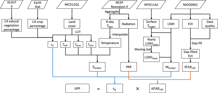
The objective of this study is to develop a new global GPP dataset that overcomes the limitation of MOD17. This dataset, dubbed VPM GPP V20, is based on an improved LUE theory which uses the energy absorbed by chlorophyll, and implemented to the entire globe during the MODIS era. The VPM algorithm utilized remotely sensed datasets together with reanalysis climate dataset and land cover classification. The schematic workflow of the VPM algorithm is shown in Fig. 1 and is described in detail in the Methods section. This dataset can serve as an alternative to MOD17 GPP product for regional and global carbon cycle studies.

Figure 1. Datasets and workflow of VPM to calculate GPP.

This figure is modified from ref. 34. ISLSCP II: International Satellite Land Surface Climatology Project, Initiative II; MODIS: Moderate Resolution Imaging Spectroradiometer; NCEP: National Centers for Environmental Prediction; EVI: enhanced vegetation index; LSWI: land surface water index; LST: land surface temperature; LUT: look-up table; T_day: daytime air temperature; T_night: nighttime land surface temperature; ε₀: maximum light use efficiency; T_opt: optimal temperature for photosynthesis; T_max: maximum temperature for photosynthesis; T_min: minimum temperature for photosynthesis; LSWI_max: maximum LSWI during the growing season. T_scalar: temperature limitation for photosynthesis; PAR: photosynthetically active radiation; W_scalar: water limitation for photosynthesis; fPAR_chl; fraction of PAR absorbed by chlorophyll; APAR_chl: absorbed PAR by chlorophyll.

Methods

Data processing

We used multiple datasets as the input of VPM. All datasets being used are summarized in Table 1, and detailed processing methods are described below.

Table 1. Input datasets used to drive vegetation photosynthesis model (VPM) and their specifications.

Data source	Dataset	Derived variables	Original spatial resolution	Original temporal resolution	Reference URL
For acronyms please refer to captions in Fig. 1.
MODIS	MOD09A1 C6	EVI, LSWI	500 m	8-day	https://doi.org/10.5067/modis/mod09a1.006
	MYD11A2 C6	Nighttime LST (01:30 am overpass)	1 km	8-day	https://doi.org/10.5067/modis/myd11a2.006
	MCD12Q1 C51	Land cover type	500 m	Annual	https://lpdaac.usgs.gov/dataset_discovery/modis/modis_products_table/mcd12q1
NCEP-reanalysis II	Daily maximum/minimum air temperature	Daytime temperature	~1.875°×2°	daily	http://www.cpc.ncep.noaa.gov/products/wesley/reanalysis2/kana/reanl2-1.htm
	Radiation	Daily mean PAR	~1.875°×2°	daily	http://www.cpc.ncep.noaa.gov/products/wesley/reanalysis2/kana/reanl2-1.htm
Earth Stat	Major crop types distribution	C4 crop percentage	0.083°	invariant	http://www.earthstat.org/data-download/
ISLSCP II	C4 vegetation percentage map	C4 grassland percentage	1°×1°	invariant	https://doi.org/10.3334/ORNLDAAC/932

Vegetation indices and gap-filling

Enhanced Vegetation Index (EVI)³⁶ and Land Surface Water Index (LSWI)³⁷ are two major inputs for the VPM model, both of which are calculated from the MOD09A1 C6 500 m 8-day land surface reflectance dataset. To generate a continuous GPP product, there are two types of data gaps we need to consider: (1) missing observations: for some tiles at some DOY, e.g., year 2001, DOY 169, 177, because of the sensor calibration, no observations were acquired during those period; (2) bad-quality data: the data quality of this remote sensing reflectance measurement is often affected by the atmospheric conditions (e.g., cloud, aerosols), a rigorous quality check and gap-filling algorithm is required to generate a reliable time series of VI data for model simulation. Since EVI values are often lower if clouds or aerosols exist, while LSWI may be slightly higher, we used different strategies to gap-fill these two vegetation indices.

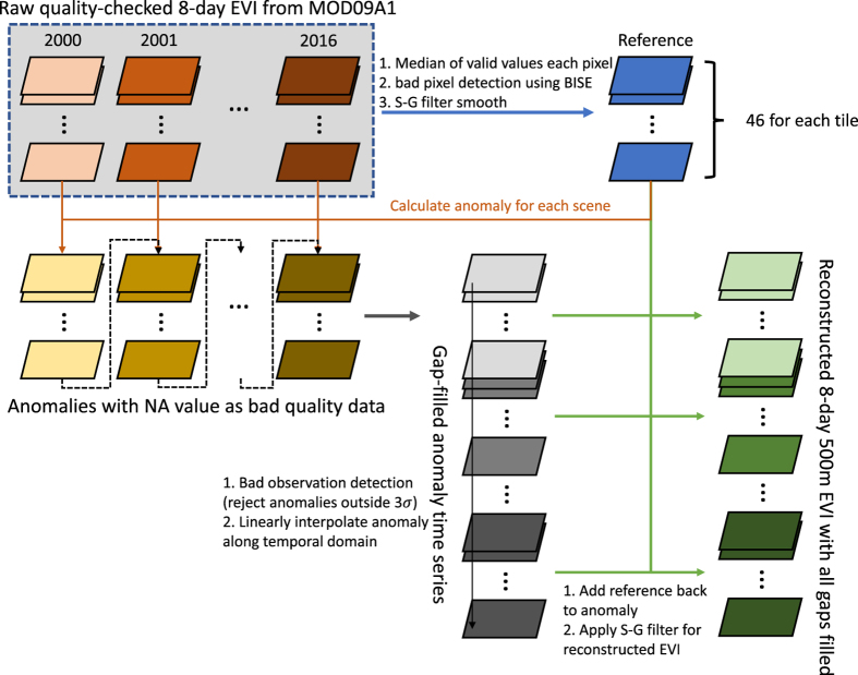
The raw EVI calculated from the reflectance was first masked for all cloud, cloud shadow and aerosol affected regions based on the quality assurance (QA) layer in the MOD09A1 dataset (MOD35 cloud=‘clear’ (bit 0–1 equals ‘00’); aerosol quantity=‘low’ or ‘average’ (bit 6–7 equals ‘01’ or ‘10’))⁸ and then filled with an advanced gap-filling algorithm (Fig. 2). The median values of valid data for each day of year (DOY) across 17 years (2000–2016) were chosen as the reference for seasonal pattern. Under extreme conditions, some bad quality data may not be identified through the QA check, these data usually have a lower value and can be detected using the Best Index Slope Extraction algorithm³⁸. After this process, gaps were filled with a linear interpolation and smoothed using a Savitzky-Golay filter. The reference will serve as a reliable baseline of the seasonal variation of EVI for each pixel. The novelty of this method is that, instead of linearly interpolate the EVI to fill the gaps within each year, we filled the gaps in seasonal anomalies (seasonal EVI−reference). This allows us to give a robust estimation when there is long period of missing/bad data during which EVI changes dramatically (Supplementary Information, Supplementary Fig. S1). To reconstruct the gap-filled EVI, we calculated the differences between EVI for one specific year and the corresponding DOY reference. The differences with missing values (generated by the quality check) were then gap filled and smoothed in the temporal domain. These gap-filled differences were added back to the reference to reconstruct the gap-filled and smoothed EVI. Using this method, we not only filled bad observations caused by atmospheric conditions, but also reconstructed the EVI for periods when no observations were made by the Terra satellite, e.g., in the year 2000 before DOY 49.

Figure 2. Flowchart showing the gap-filling and smoothing algorithm for reconstructing continuous EVI for 2000 to 2016.

Different monochromatic colors represent different intermediate outputs, with different shades indicating different years.

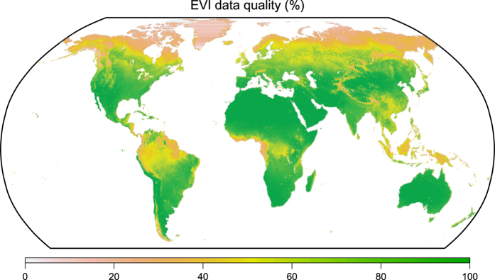
Figure 3 shows the average percentage of the good EVI data for the entire period. Gap-filled EVI data mostly locates in boreal regions, which is caused by high frequency of snow, clouds and aerosols; and tropical regions, which is caused by clouds and aerosols. No significant trend in data quality was found for most areas during 2002–2015 (Supplementary Information, Supplementary Fig. S2).

Figure 3. Average percentage of good EVI data (not gap-filled) for 2000–2016.

For LSWI which also suffers from missing observations in 2000, 2001 and 2016, we used the corresponding DOY scenes in 2001, 2002 and 2015 to fill the gaps in 2000, 2001 and 2016, respectively. This approach may introduce uncertainties due to the year to year variation of vegetation water condition and the biased estimation when cloud or snow exist. However, we believe it has limited impact on the GPP estimates since LSWI was not a factor for GPP but was used to indicate water stress. When cloud and snow exist, it usually corresponds to a higher LSWI value and the water stress is limited. We did not use the same algorithm for LSWI gap-filling because (1) LSWI is sensitive to surface water (snow, ice, flooding, etc.), and will exhibit a higher value which cannot be removed by using the BISE algorithm. (2) LSWI has higher variance which contains information of water stress and using this gap-filling algorithm may smooth this information. (3) atmospheric corruptions have limited effects on LSWI than EVI^8,30. Future studies may consider using vegetation optical depth (VOD) as an indicator of water stress and upscale to higher spatial resolution³⁹.

C4 percentage for cropland and natural vegetation

C3/C4 plants have substantial differences in utilizing solar energies⁴⁰. C4 plants do not have photorespiration and are less likely to have the light saturation effect⁴¹. Many previous studies have shown that C3/C4 plants should be treated differently in LUE models⁴². Herein lies one of the major causes for underestimation of GPP in cropland, since many models do not consider the C3/C4 difference.

Our previous VPM GPP product for North America did take C3 and C4 crop into consideration³⁴. However, because of the data availability and spatial and temporal coverage, we did not used the Cropland Data Layer but made a simple assumption that the C3/C4 species are half-half for all cropland pixels. This is not accurate since, for example, the Mid-West corn belt grows much more corn (C4) than the Mississippi river basin. Since we aim to develop a global GPP product in this study, we use two static C4 vegetation maps (one for cropland, one for natural vegetation) for the entire globe. Although these maps are low in spatial resolution (Table 1) and lack inter-annual variation, they provide the best estimates of C4 vegetation distribution based on our current knowledge^43,44. C4 crop and natural vegetation are considered separately. For C4 crop, we used the Earth Stat global major crop type distribution for the year 2000⁴⁴. Among 19 major crop types, 4 are C4 crops (corn, millet, sorghum, sugarcane). This dataset provides the plant area percentage of each crop type for each 0.083 degree gridcell, through which we calculated the C4/C3 crop ratio:

$$\begin{array}{}\text{(2)}& {\mathrm{Ratio}}_{\mathrm{C}4}=\frac{\mathrm{C}4\mathrm{crop}\mathrm{percentage}}{\mathrm{Total}\mathrm{crop}\mathrm{percentage}}\end{array}$$

where the Total crop percentage for the 0.083 gridcell was calculated from the MODIS landcover dataset (MCD12C1 C55). Within each 0.083 degree gridcell, all 500-m cropland pixels were considered to have a fixed C3/C4 crop ratio which allowed us to calculate the LUE using the area-weighted average of C3 and C4 LUE. However, this assumption introduces uncertainty when comparing simulated GPP with GPP estimates from cropland flux towers, since most sites are surrounded by either pure C3 or C4 crop. When averaged over a larger scale however, this mismatch may be negligible. We used the ISLSCP II C4 vegetation map for natural C4 vegetation distribution⁴³ and assumed that all grassland, savannas, woody savannas and wetland within each 1°×1° gridcell share the same C3/C4 ratio. The corresponding LUE for these C3/C4 mixed pixels can be calculated based on their area-weighted averages.

Climate data

For the global GPP simulation, we used the NCEP reanalysis II dataset. The daily downward shortwave radiation flux at surface (dswrf in Wm⁻²) was averaged over 8 days to match the model simulation interval. We used the average of daily maximum temperature (tmax.2m) and the daily mean temperature (air.2m) as daytime temperature and it was then averaged over each 8-day period. The aggregated datasets were in Gaussian grid (192×96) and further downscaled to the 500-m resolution using the same method that was described in previous publications^21,34.

Vegetation photosynthesis model (VPM) description

The VPM model follows the light use efficiency scheme and estimates GPP as the product of light absorption by chlorophyll of the vegetation (APAR_chl) and the efficiency (ε_g) that converts the absorbed energy to carbon fixed by plants through photosynthesis:

$$\begin{array}{}\text{(3)}& \mathrm{GPP}={\mathrm{APAR}}_{\mathrm{chl}}\times {\mathit{\epsilon }}_{\mathrm{g}}\end{array}$$

where APAR_chl is calculated as a product of photosynthetically active radiation (PAR) and the fraction of PAR absorbed by chlorophyll (fPAR_chl):

$$\begin{array}{}\text{(4)}& {\mathrm{APAR}}_{\mathrm{chl}}=\mathrm{PAR}\times {\mathrm{fPAR}}_{\mathrm{chl}}\end{array}$$

The fPAR_chl is calculated as a linear function of EVI, which is modified from previous model framework³²:

$$\begin{array}{}\text{(5)}& {\mathrm{fPAR}}_{\mathrm{chl}}=\left(\mathrm{EVI}-0.1\right)\times 1.25\end{array}$$

The coefficients 0.1 and 1.25 are used to adjust for sparsely vegetated or barren land and have been validated using the solar-induced chlorophyll fluorescence data (data not shown). ε_g in equation (3) is down-regulated by temperature limitation (T_scalar) and water stress (W_scalar) from its maximum value (ε₀) which only differs by C3/C4 photosynthesis pathways:

$$\begin{array}{}\text{(6)}& {\mathit{\epsilon }}_{\mathrm{g}}={\mathit{\epsilon }}_0\times {\mathrm{T}}_{\mathrm{scalar}}\times {\mathrm{W}}_{\mathrm{scalar}}\end{array}$$

Both T_scalar and W_scalar range from 0 to 1 and can be calculated as follows:

$$\begin{array}{}\text{(7)}& {\mathrm{T}}_{\mathrm{scalar}}=\frac{\left(\mathrm{T}-{\mathrm{T}}_{\max }\right)\times \left(\mathrm{T}-{\mathrm{T}}_{\min }\right)}{\left(\mathrm{T}-{\mathrm{T}}_{\max }\right)\times \left(\mathrm{T}-{\mathrm{T}}_{\min }\right)-{(\mathrm{T}-{\mathrm{T}}_{\mathrm{opt}})}^2}\end{array}$$

$$\begin{array}{}\text{(8)}& {\mathrm{W}}_{\mathrm{scalar}}=\frac{1+\mathrm{LSWI}}{1+{\mathrm{LSWI}}_{\max }}\end{array}$$

Where the T, T_max, T_min and T_opt refer to the daytime mean temperature, maximum, minimum, and optimum temperature for photosynthesis, respectively. The last three parameters are biome-based and can be obtained from a look-up table (Table 2). The land cover product from MODIS (MOD12Q1) is used to provide biome information since this is the only annual land cover product with high spatial resolution and global coverage. The uncertainty of the land cover classification is not assessed but is supposed to have limited effect on the final GPP estimation since it only directly affects the temperature scalar and indirectly affects ε₀. LSWI_max is the maximum LSWI during the snow-free period for each pixel each year. To eliminate potential bias, a temporal smoothing using nearby four years (two years before, two years after) is applied and calculates the second largest LSWI_max within this five-year period³⁴.

Table 2. Biome specific lookup-table.

IGBP class	ε0 (g C/mol APAR)	Tmin (°C)	Tmax (°C)	Topt (°C)
This table is adopted from ref. 34, where the ε0 values are from multiple site level studies30,33,66,67, and the temperature related parameters are adopted from Terrestrial Ecosystem Model68,69.
ENF: evergreen needleleaf forest; EBF: evergreen broadleaf forest; DNF: deciduous needleleaf forest; DBF: deciduous broadleaf forests; MF: mixed forest; CSH: closed shrublands; OSH: open shrublands; WSA: woody savannas; SAV: savannas; GRA: grassland; WET: wetland; CRO: cropland; URB: Urban; NVM: cropland/natural vegetation mosaic.
ENF	0.42	−1	40	20
EBF	0.42	−2	48	28
DNF	0.42	−1	40	20
DBF	0.42	−1	40	20
MF	0.42	−1	48	19
CSH	0.42	−1	48	25
OSH	0.42	1	48	31
WSA	0.42	−1	48	24
SAV	0.42 (C3) 0.63 (C4)	1	48	30
GRA	0.42 (C3) 0.63 (C4)	0	48	27
WET	0.42 (C3) 0.63 (C4)	−1	40	20
CRO	0.42 (C3) 0.63 (C4)	−1	48	30
URB	0.42	0	48	27
CNV	0.42 (C3) 0.63 (C4)	0	48	27

Code availability

The code for EVI gap-filling and VPM algorithms are available at https://github.com/zhangyaonju/Global_GPP_VPM_NCEP_C3C4.

Data Records

The original VPM GPP V20 dataset is available at 500 m spatial resolution and 8-day temporal resolution. The entire earth land surface is divided into 290 subregions (tiles) under the sinusoidal projection. There are 46 GeoTiff files for each year each tile, each of which represents GPP for an 8-day average. The units are all in g C m⁻² day⁻¹ with a scalar factor of 0.001. Each file is also associated with a data quality layer: a Boolean value indicates whether the EVI is from the raw data (0) or gap-filled (1). We also provide two coarser spatial resolutions at 0.05°×0.05° and 0.5°×0.5° with a longitude-latitude projection under WGS84 datum. Three temporal resolutions, i.e., 8-day, monthly and annual, are available for 0.05°×0.05° and 0.5°×0.5° spatial resolution products. The units are g C m⁻² day⁻¹, g C m⁻² month⁻¹, and g C m⁻² year⁻¹, respectively. GPP products at 0.05°×0.05° and 0.5°×0.5° spatial resolutions can be accessed at (Data Citation 1); the raw 500 m 8-day GPP product together with the data quality layer can be accessed at (Data Citation 2). Because of the state-of-the-art gap-filling and smoothing algorithms applied, we can provide a continuous spatial temporal GPP estimate with no missing tiles.

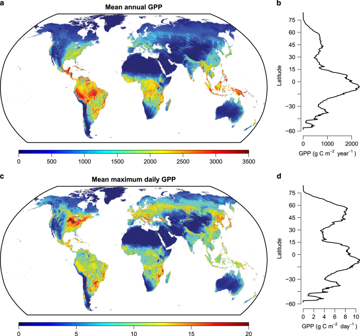
The global GPP estimation for the period 2000 to 2016 ranges from 121.60 to 129.42 Pg C year⁻¹ with an increasing rate of ~0.39 Pg C year⁻². The highest annual GPP occurs mostly in tropical regions, especially in the Amazon and Southeast Asia (Fig. 4a). This corresponds to the highest peak in annual GPP around the equator (Fig. 4b). The maximum daily GPP however, shows its highest value in the Midwest region of the United States. Other crop planting regions, e.g., central Europe, Northeast China, Southeast Africa and South America also show relatively high maximum daily GPP. High maximum productivity in these regions creates another peak around 50°N (Fig. 4d).

Figure 4. Spatial pattern of annual and maximum daily GPP for 2000–2016.

(a) average annual GPP, (c) maximum daily GPP, latitudinal pattern of (b) average annual GPP, and (d) maximum daily GPP. Annual total GPP and maximum daily GPP within a year were averaged over the period of 2000 to 2016.

All other continents except South America and Oceania exhibit an increasing trend of annual GPP over the past 17 years (Table 3). The increasing rate is highest for Europe (0.89% year⁻¹), followed by Asia (0.64% year⁻¹), North America (0.61% year⁻¹), and Africa (0.21% year⁻¹). Annual GPP for Oceania did not show much change throughout the study period while South America experienced a significant decrease (−0.19% year⁻¹).

Table 3. Continental and global total GPP for each year.

Year	Africa	Asia	Europe	North America	South America	Oceania	Global total
Units are in Pg C year−1.
2000	27.43	29.82	8.50	16.69	33.72	5.44	121.60
2001	27.69	30.52	8.64	17.22	33.43	4.96	122.46
2002	27.62	31.64	8.82	16.46	34.05	4.17	122.76
2003	27.57	31.18	8.54	17.33	34.02	4.29	122.93
2004	27.84	30.86	8.83	17.81	34.61	4.79	124.74
2005	26.93	31.00	8.90	17.88	34.27	4.43	123.41
2006	28.62	31.50	8.86	17.37	34.92	4.74	126.02
2007	28.20	31.76	9.04	18.03	33.28	4.39	124.70
2008	28.27	31.39	9.10	17.47	33.07	4.52	123.82
2009	28.80	31.82	9.07	17.23	33.92	4.54	125.38
2010	28.30	31.80	8.88	18.14	33.46	5.32	125.90
2011	28.54	32.21	9.43	17.26	33.52	5.82	126.79
2012	28.23	32.26	9.11	18.19	32.90	4.98	125.66
2013	29.09	33.00	9.48	17.89	32.89	4.48	126.81
2014	29.41	33.13	9.67	18.08	33.33	4.73	128.35
2015	28.02	34.42	9.79	19.05	33.73	4.42	129.42
2016	27.19	33.43	10.08	19.10	33.10	4.79	127.70

Technical Validation

Comparison against eddy covariance flux tower

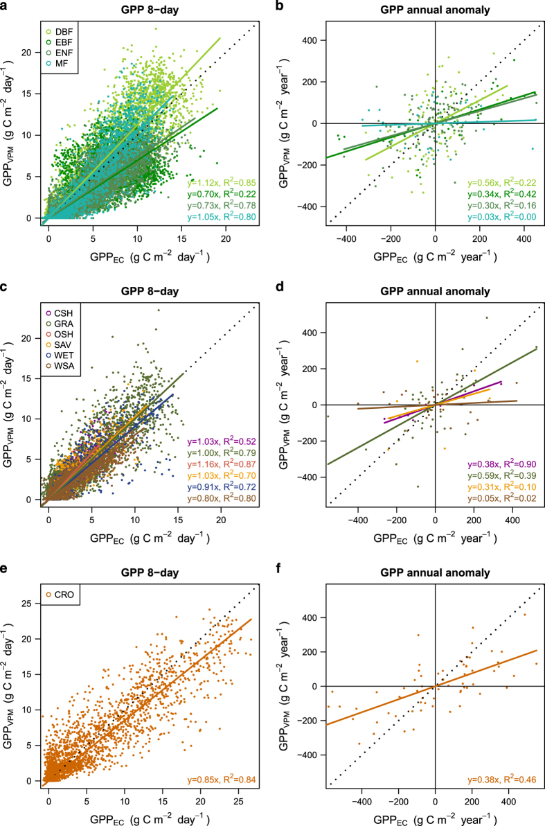
This GPP dataset was validated against 113 eddy covariance flux towers across the globe. These flux towers data were obtained from the FLUXNET 2015 Tier 1 dataset (2016 November release, http://fluxnet.fluxdata.org/data/fluxnet2015-dataset/), and only a small portion (23 out of 136) was excluded due to inconsistency between the flux tower footprint and MODIS pixels (Supplementary Information,Supplementary Table S1). GPP from the flux tower was calculated as an average from both daytime and nighttime partition methods after a rigorous data quality check. The validation was carried out at two scales: (1) at spatial and seasonal scale, we used all 8-day GPP estimates for all sites-years (n=28,378) and (2) at interannual scale, we calculated annual GPP anomalies for long-term sites from both EC estimates and VPM (more than 5 years of observation between 2000 and 2016, n=479) (Fig. 5).

Figure 5. GPP validation against eddy covariance measurements for different biome types.

Comparison of GPP for (a,b) forest, (c,d) non-forest and (e,f) cropland at 8-day scale across sites, and at annual scale in anomalies. Each point in (a,c,e) represents GPP estimates from VPM and EC for an 8-day period from one site; each point in (b,d,f) represents annual GPP estimates anomalies (GPP for one year minus GPP average over years for this site) for one year from one site; only sites with more than 5 years’ observations were used for annual anomaly comparison.

The overall accuracy of the VPM GPP V20 dataset is relatively high with an R² of 0.74 and a low RMSE of 2.08 g C m⁻² day⁻¹. A complete list of sites used and GPP comparisons is available in the Supplementary Information (Supplementary Table S1). For individual biome types, the VPM GPP product underestimated evergreen forest (~27% and 30% for ENF and EBF, respectively) and slightly underestimated cropland (~15%). For other biome types, the VPM GPP did not show a systematic bias for the spatial seasonal variation. Except ENF and CSH, most biome types showed relative high R² values (>0.7) which means VPM GPP captures well the spatial and seasonal variations. In terms of interannual variation, VPM GPP did not show much agreement with EC-based GPP estimates. Across all biome types, VPM GPP showed less inter-annual variation compared with that from the EC tower. The R² is low (<0.5) for most biome types. This low consistency in interannual variation may be caused by insensitivity of stress factors of VPM at an interannual scale, ecosystem memory effects which is not taken into consideration in VPM, and uncertainties in both GPP estimates.

Comparison with other GPP datasets

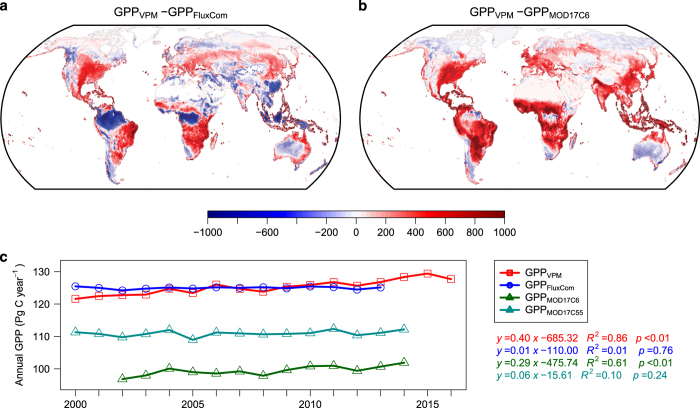
We also compared our GPP dataset with some other data-driven GPP products, e.g., FluxCom GPP, MOD17 (both C55 and C6). VPM showed higher annual GPP estimates in eastern and central US, mid-latitude Eurasia, and subtropical region in South America and Africa (Fig. 6a). These regions are mostly dominated by C4 cropland or grassland. VPM GPP is lower in tropical rainforest. When compared with MOD17C6, VPM gave higher estimations for most mid- to low-latitude regions, which is consistent with a recent study suggesting that MOD17C6 largely underestimates GPP for most ecosystems²⁰.

Figure 6. Comparison of GPP_VPM with other GPP products.

Mean annual GPP difference between VPM and (a) FluxCom^14,61 (for the period 2000–2013) and (b) MOD17A2H C6⁶² (MOD17C6 for the period 2002–2014) and (c) annual total GPP from VPM, FluxCom, MOD17 (both C6⁶² and C55 version²²). Units for (a,b) are g C m⁻² year⁻¹. GPP_MOD17C6 was not available for year 2000, 2001 and 2015 because of the missing tiles in the data distribution center. All comparisons were conducted at 0.5°×0.5° spatial resolution.

The average global annual GPP estimates are similar in value for VPM and FluxCom, both around 125 Pg C year⁻¹, though VPM showed a significant increasing trend (0.39 Pg C year⁻²) while FluxCom is almost stable during the past 14 years (Fig. 6c). Both MOD17 products showed lower GPP estimates, with a difference of ~14 Pg C year⁻¹ for MOD17C55 and ~26 Pg C year⁻¹ for MOD17C6, in comparison with VPM GPP. The C6 version of MOD17 also showed a significant increasing trend (0.29 Pg C year⁻²) that did not appear in the C55 version. This difference may be caused by using different climate data (GMAO/NASA (Global Modeling and Assimilation Office/National Aeronautics and Space Administration) and NCEP Reanalysis II) or the corrected sensor degradation effect in MODIS C6 data^45,46.

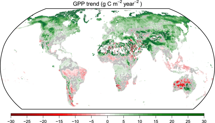
We also calculated the spatial pattern of GPP trend using the 0.5°×0.5° 8-day dataset as a further validation (Fig. 7). This spatial pattern is consistent with many previous studies: (1) high latitude regions and Qinghai Tibet Plateau experienced a continuous increasing GPP caused by warming and extended growing season^47–50; (2) afforestation in Northern China^51,52 and vegetation greening in southern Sahara Desert^53,54 also lead to an increase in GPP; (3) Tropical forest in southeast Asia⁵⁵ and southern part of Amazon⁵⁶ where deforestation happened exhibited a decreasing trend of GPP.

Figure 7. The GPP trend estimated from the seasonal Theil-Sen’s slope estimator^63,64.

Grey area indicates no significant trend at 0.05 level according to the seasonal Mann-Kendall test⁶⁵. Very high and low values in Arabian Peninsula and central Australia may be caused by artifacts of the seasonal Theil-Sen’s slope method and is not evident in linear regression.

Overall, GPP_VPM provides a reliable GPP estimation for non-forest natural vegetation and cropland by considering the C3/C4 vegetation ratio⁵⁷. The underestimation for ENF and EBF may be related to the higher light use efficiency for diffused radiation⁵⁸, but requires further testing. The total global GPP estimation is close to previous studies using different approaches^59,60, and the trend of annual GPP increase are also in line with some other recent reports⁴.

Usage Notes

The GPP for gridcells in coastal regions (in 0.05°×0.05 and 0.5°×0.5° spatial resolution products) are averaged over the entire gridcell but land only, therefore, the land area fraction is not needed when calculating the regional sum.

Additional information

How to cite this article: Zhang, Y. et al. A global moderate resolution dataset of gross primary production of vegetation for 2000–2016. Sci. Data 4:170165 doi: 10.1038/sdata.2017.165 (2017).

Publisher’s note: Springer Nature remains neutral with regard to jurisdictional claims in published maps and institutional affiliations.

References

- Le Quéré C. et al. Global Carbon Budget 2016. Earth Syst. Sci. Data 8, 605–649 (2016). [Google Scholar]
- Hartmann D., Tank A. & Rusticucci M. IPCC fifth assessment report, climate change 2013: The physical science basis. IPCC AR5 31–39 (2013). [Google Scholar]
- Reichstein M. et al. Climate extremes and the carbon cycle. Nature 500, 287–295 (2013). [DOI] [PubMed] [Google Scholar]
- Keenan T. F. et al. Recent pause in the growth rate of atmospheric CO2 due to enhanced terrestrial carbon uptake. Nat. Commun 7, 13428 (2016). [DOI] [PMC free article] [PubMed] [Google Scholar]
- Ciais P. et al. Europe-wide reduction in primary productivity caused by the heat and drought in 2003. Nature 437, 529–533 (2005). [DOI] [PubMed] [Google Scholar]
- Zhang Y. et al. Precipitation and carbon-water coupling jointly control the interannual variability of global land gross primary production. Sci. Rep. 6, 39748 (2016). [DOI] [PMC free article] [PubMed] [Google Scholar]
- Ahlstrom A. et al. The dominant role of semi-arid ecosystems in the trend and variability of the land CO2 sink. Science 348, 895–899 (2015). [DOI] [PubMed] [Google Scholar]
- Zhang Y. et al. Canopy and physiological controls of GPP during drought and heat wave. Geophys. Res. Lett. 43, 3325–3333 (2016). [Google Scholar]
- Farquhar G. D., Caemmerer S. V. & Berry J. A. A Biochemical-Model of Photosynthetic Co2 Assimilation in Leaves of C-3 Species. Planta 149, 78–90 (1980). [DOI] [PubMed] [Google Scholar]
- Pury D. D. & Farquhar G. Simple scaling of photosynthesis from leaves to canopies without the errors of big‐leaf models. Plant Cell Environ. 20, 537–557 (1997). [Google Scholar]
- Zhang Y. et al. Development of a coupled carbon and water model for estimating global gross primary productivity and evapotranspiration based on eddy flux and remote sensing data. Agr. Forest Meteorol. 223, 116–131 (2016). [Google Scholar]
- Running S. W. et al. A continuous satellite-derived measure of global terrestrial primary production. Bioscience 54, 547–560 (2004). [Google Scholar]
- Xiao J. et al. Estimation of net ecosystem carbon exchange for the conterminous United States by combining MODIS and AmeriFlux data. Agr. Forest Meteorol. 148, 1827–1847 (2008). [Google Scholar]
- Tramontana G. et al. Predicting carbon dioxide and energy fluxes across global FLUXNET sites with regression algorithms. Biogeosciences 13, 4291–4313 (2016). [Google Scholar]
- Guanter L. et al. Global and time-resolved monitoring of crop photosynthesis with chlorophyll fluorescence. Proc. Nat. Acad. Sci. USA 111, E1327–E1333 (2014). [DOI] [PMC free article] [PubMed] [Google Scholar]
- Monteith J. L. Solar-Radiation and Productivity in Tropical Ecosystems. J. Appl. Ecol. 9, 747–766 (1972). [Google Scholar]
- Song C. H., Dannenberg M. P. & Hwang T. Optical remote sensing of terrestrial ecosystem primary productivity. Prog. Phys. Geog. 37, 834–854 (2013). [Google Scholar]
- Turner D. P. et al. Evaluation of MODIS NPP and GPP products across multiple biomes. Remote Sens. Environ. 102, 282–292 (2006). [Google Scholar]
- Zhang F. et al. Evaluating spatial and temporal patterns of MODIS GPP over the conterminous U.S. against flux measurements and a process model. Remote Sens. Environ. 124, 717–729 (2012). [Google Scholar]
- Wang L. et al. Evaluation of the Latest MODIS GPP Products across Multiple Biomes Using Global Eddy Covariance Flux Data. Remote Sens 9, 418 (2017). [Google Scholar]
- Zhao M., Heinsch F. A., Nemani R. R. & Running S. W. Improvements of the MODIS terrestrial gross and net primary production global data set. Remote Sens. Environ. 95, 164–176 (2005). [Google Scholar]
- Zhao M. & Running S. W. Drought-induced reduction in global terrestrial net primary production from 2000 through 2009. Science 329, 940–943 (2010). [DOI] [PubMed] [Google Scholar]
- Wu J. et al. Leaf development and demography explain photosynthetic seasonality in Amazon evergreen forests. Science 351, 972–976 (2016). [DOI] [PubMed] [Google Scholar]
- Kattge J., Knorr W., Raddatz T. & Wirth C. Quantifying photosynthetic capacity and its relationship to leaf nitrogen content for global-scale terrestrial biosphere models. Glob. Change Biol. 15, 976–991 (2009). [Google Scholar]
- Houborg R., Cescatti A., Migliavacca M. & Kustas W. P. Satellite retrievals of leaf chlorophyll and photosynthetic capacity for improved modeling of GPP. Agr. Forest Meteorol. 177, 10–23 (2013). [Google Scholar]
- Piñeiro G., Oesterheld M. & Paruelo J. M. Seasonal Variation in Aboveground Production and Radiation-use Efficiency of Temperate rangelands Estimated through Remote Sensing. Ecosystems 9, 357–373 (2006). [Google Scholar]
- Xu L. & Baldocchi D. D. Seasonal trends in photosynthetic parameters and stomatal conductance of blue oak (Quercus douglasii) under prolonged summer drought and high temperature. Tree Physiol. 23, 865–877 (2003). [DOI] [PubMed] [Google Scholar]
- Zhang Q. Y. et al. Can a satellite-derived estimate of the fraction of PAR absorbed by chlorophyll (FAPAR(chl)) improve predictions of light-use efficiency and ecosystem photosynthesis for a boreal aspen forest? Remote Sens. Environ. 113, 880–888 (2009). [Google Scholar]
- Zhang Q. Y. et al. Estimation of crop gross primary production (GPP): fAPAR(chl) versus MOD15A2 FPAR. Remote Sens. Environ. 153, 1–6 (2014). [Google Scholar]
- Jin C. et al. Phenology and gross primary production of two dominant savanna woodland ecosystems in Southern Africa. Remote Sens. Environ. 135, 189–201 (2013). [Google Scholar]
- Xiao X. et al. Satellite-based modeling of gross primary production in an evergreen needleleaf forest. Remote Sens. Environ. 89, 519–534 (2004). [Google Scholar]
- Xiao X. et al. Modeling gross primary production of temperate deciduous broadleaf forest using satellite images and climate data. Remote Sens. Environ. 91, 256–270 (2004). [Google Scholar]
- Wang J. et al. Canopy and climate controls of gross primary production of Mediterranean-type deciduous and evergreen oak savannas. Agr. Forest Meteorol. 226-227, 132–147 (2016). [Google Scholar]
- Zhang Y. et al. Consistency between sun-induced chlorophyll fluorescence and gross primary production of vegetation in North America. Remote Sens. Environ. 183, 154–169 (2016). [Google Scholar]
- Zhou S. et al. Dominant role of plant physiology in trend and variability of gross primary productivity in North America. Sci. Rep. 7, 41366 (2017). [DOI] [PMC free article] [PubMed] [Google Scholar]
- Huete A. et al. Overview of the radiometric and biophysical performance of the MODIS vegetation indices. Remote Sens. Environ. 83, 195–213 (2002). [Google Scholar]
- Xiao X. et al. Observation of flooding and rice transplanting of paddy rice fields at the site to landscape scales in China using VEGETATION sensor data. Int. J. Remote Sens. 23, 3009–3022 (2002). [Google Scholar]
- Viovy N., Arino O. & Belward A. The Best Index Slope Extraction (BISE): A method for reducing noise in NDVI time-series. Int. J. Remote Sens. 13, 1585–1590 (1992). [Google Scholar]
- Konings A. G. & Gentine P. Global variations in ecosystem-scale isohydricity. Glob. Change Biol. 23, 891–905 (2017). [DOI] [PubMed] [Google Scholar]
- Jin C. et al. Effects of in-situ and reanalysis climate data on estimation of cropland gross primary production using the Vegetation Photosynthesis Model. Agr. Forest Meteorol. 213, 240–250 (2015). [Google Scholar]
- Collatz G. J., Ribas-Carbo M. & Berry J. A. Coupled Photosynthesis-Stomatal Conductance Model for Leaves of C4 Plants. Aust. J. Plant Physiol. 19, 519–538 (1992). [Google Scholar]
- Yan H. et al. Improved global simulations of gross primary product based on a new definition of water stress factor and a separate treatment of C3 and C4 plants. Ecol. Model. 297, 42–59 (2015). [Google Scholar]
- Still C. J., Berry J. A., Collatz G. J. & DeFries R. S. Global distribution of C3and C4vegetation: Carbon cycle implications. Global Biogeochem. Cycles 17, 1006 (2003). [Google Scholar]
- Monfreda C., Ramankutty N. & Foley J. A. Farming the planet: 2. Geographic distribution of crop areas, yields, physiological types, and net primary production in the year 2000. Global Biogeochem. Cycles 22, GB1022 (2008). [Google Scholar]
- Zhang Y., Song C., Band L. E., Sun G. & Li J. Reanalysis of global terrestrial vegetation trends from MODIS products: Browning or greening? Remote Sens. Environ. 191, 145–155 (2017). [Google Scholar]
- Lyapustin A. et al. Scientific impact of MODIS C5 calibration degradation and C6+ improvements. Atmos. Meas. Tech 7, 4353–4365 (2014). [Google Scholar]
- Zhang G., Zhang Y., Dong J. & Xiao X. Green-up dates in the Tibetan Plateau have continuously advanced from 1982 to 2011. Proc. Nat. Acad. Sci. USA 110, 4309–4314 (2013). [DOI] [PMC free article] [PubMed] [Google Scholar]
- Shen M. et al. Evaporative cooling over the Tibetan Plateau induced by vegetation growth. Proc. Nat. Acad. Sci. U.S.A 112, 9299–9304 (2015). [DOI] [PMC free article] [PubMed] [Google Scholar]
- Zhu Z. et al. Greening of the Earth and its drivers. Nat. Clim. Change 6, 791–795 (2016). [Google Scholar]
- Forkel M. et al. Enhanced seasonal CO2 exchange caused by amplified plant productivity in northern ecosystems. Science 351, 696–699 (2016). [DOI] [PubMed] [Google Scholar]
- Zhang Y. et al. Multiple afforestation programs accelerate the greenness in the ‘Three North’ region of China from 1982 to 2013. Ecol. Indic. 61, 404–412 (2016). [Google Scholar]
- Feng X., Fu B., Lu N., Zeng Y. & Wu B. How ecological restoration alters ecosystem services: an analysis of carbon sequestration in China's Loess Plateau. Sci. Rep. 3, 2846 (2013). [DOI] [PMC free article] [PubMed] [Google Scholar]
- Dardel C. et al. Re-greening Sahel: 30 years of remote sensing data and field observations (Mali, Niger). Remote Sens. Environ. 140, 350–364 (2014). [Google Scholar]
- Brandt M. et al. Ground- and satellite-based evidence of the biophysical mechanisms behind the greening Sahel. Glob. Change Biol. 21, 1610–1620 (2015). [DOI] [PubMed] [Google Scholar]
- Miettinen J., Shi C. & Liew S. C. Deforestation rates in insular Southeast Asia between 2000 and 2010. Glob. Change Biol. 17, 2261–2270 (2011). [Google Scholar]
- Sy V. D. et al. Land use patterns and related carbon losses following deforestation in South America. Environ. Res. Lett. 10 (2015). [Google Scholar]
- Yuan W. et al. Uncertainty in simulating gross primary production of cropland ecosystem from satellite-based models. Agr. Forest Meteorol. 207, 48–57 (2015). [Google Scholar]
- Mercado L. M. et al. Impact of changes in diffuse radiation on the global land carbon sink. Nature 458, 1014–1017 (2009). [DOI] [PubMed] [Google Scholar]
- Beer C. et al. Terrestrial gross carbon dioxide uptake: global distribution and covariation with climate. Science 329, 834–838 (2010). [DOI] [PubMed] [Google Scholar]
- Ciais P. et al. A three-dimensional synthesis study of δ18O in atmospheric CO2: 1. Surface fluxes. J. Geophys. Res. Atmos 102, 5857–5872 (1997). [Google Scholar]
- Jung M. et al. Compensatory water effects link yearly global land CO2 sink changes to temperature. Nature 541, 516–520 (2017). [DOI] [PubMed] [Google Scholar]
- Running S., Mu Q. & Zhao M. MOD17A2H MODIS/Terra Gross Primary Productivity 8-Day L4 Global 500m SIN Grid V006 (Reston, VA, USA, 2015). [Google Scholar]
- Hipel K. W. & McLeod A. I. Time series modelling of water resources and environmental systems Vol. 45 (Elsevier, 1994). [Google Scholar]
- Sen P. K. Estimates of the regression coefficient based on Kendall's tau. J. Am. Stat. Assoc 63, 1379–1389 (1968). [Google Scholar]
- Hirsch R. M., Slack J. R. & Smith R. A. Techniques of trend analysis for monthly water quality data. Water Resour. Res. 18, 107–121 (1982). [Google Scholar]
- Wagle P. et al. Sensitivity of vegetation indices and gross primary production of tallgrass prairie to severe drought. Remote Sens. Environ. 152, 1–14 (2014). [Google Scholar]
- Kalfas J. L., Xiao X., Vanegas D. X., Verma S. B. & Suyker A. E. Modeling gross primary production of irrigated and rain-fed maize using MODIS imagery and CO2 flux tower data. Agr. Forest Meteorol. 151, 1514–1528 (2011). [Google Scholar]
- Aber J. D., Reich P. B. & Goulden M. L. Extrapolating leaf CO2 exchange to the canopy: a generalized model of forest photosynthesis compared with measurements by eddy correlation. Oecologia 106, 257–265 (1996). [DOI] [PubMed] [Google Scholar]
- McGuire A. D. et al. Interactions between carbon and nitrogen dynamics in estimating net primary productivity for potential vegetation in North America. Global Biogeochem. Cycles 6, 101–124 (1992). [Google Scholar]
Associated Data
This section collects any data citations, data availability statements, or supplementary materials included in this article.
Data Citations
- Zhang Y. 2017. Figshare. https://doi.org/10.6084/m9.figshare.c.3789814
- Zhang Y. 2017. PANGAEA. https://doi.org/10.1594/PANGAEA.879560