Generalizing DTW to the multi-dimensional case requires an adaptive approach

Abstract

In recent years Dynamic Time Warping (DTW) has emerged as the distance measure of choice for virtually all time series data mining applications. For example, virtually all applications that process data from wearable devices use DTW as a core sub-routine. This is the result of significant progress in improving DTW’s efficiency, together with multiple empirical studies showing that DTW-based classifiers at least equal (and generally surpass) the accuracy of all their rivals across dozens of datasets. Thus far, most of the research has considered only the one-dimensional case, with practitioners generalizing to the multi-dimensional case in one of two ways, dependent or independent warping. In general, it appears the community believes either that the two ways are equivalent, or that the choice is irrelevant. In this work, we show that this is not the case. The two most commonly used multi-dimensional DTW methods can produce different classifications, and neither one dominates over the other. This seems to suggest that one should learn the best method for a particular application. However, we will show that this is not necessary; a simple, principled rule can be used on a case-by-case basis to predict which of the two methods we should trust at the time of classification. Our method allows us to ensure that classification results are at least as accurate as the better of the two rival methods, and, in many cases, our method is significantly more accurate. We demonstrate our ideas with the most extensive set of multi-dimensional time series classification experiments ever attempted.

1 Introduction

The research community seems to have converged on the belief that Dynamic Time Warping (DTW) is remarkably hard to beat as a time series distance measure, across a host of domain applications, and a host of tasks; including clustering, classification and similarity search (Ding et al. 2008; Papapetrou et al. 2011). Moreover, the most often cited reason for not using DTW, its relatively high time complexity, has recently become a non-issue. In particular, amortized over a subsequence search or subsequence monitoring task, DTW is slower than Euclidean Distance by less than a factor of two (Rakthanmanon et al. 2013). As a practical matter, carefully optimized DTW is much faster than all but the most carefully optimized implementations of Euclidean Distance (Aach and Church 2001). For example, a modern cell phone, using the state-of-the-art DTW subsequence monitoring algorithm (Rakthanmanon et al. 2013), can easily process streams arriving at several thousand Hertz. However, such devices only produce data at about 100Hz.

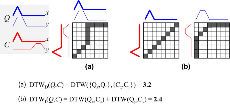
Virtually all attempts to improve time series classification in the last two decades have focused on the single-dimensional case, with the assumption that the generalization to the multi-dimensional case is trivial. There are two obvious ways DTW can be generalized to the multi-dimensional case: Fig. 1 gives a visual intuition, which we formalize later in this work. For clarity, we refer to the two methods as DTW_D and DTW_I (with _D standing for Dependent and _I for Independent).

Fig. 1.

top left Two multi-dimensional time series. a The DTW_D distance between them is 3.2. b The DTW_I distance between them is 2.4. All elements of this visual key are formally defined below

The vast majority of researchers seem to think that it makes no difference which method is used, as evidenced by the fact that they usually do not explicitly bother to tell the reader.

With some introspection we can see that there are actually several possibilities:

• There is no difference between DTW_D and DTW_I; they produce the same values for all time series.

However, we can immediately dismiss this possibility; as shown in Fig. 1, the two methods generally produce different distance values, and thus could produce different class labels if classifying an object using the Nearest Neighbor (NN) algorithm.

The next possibility seems to be the one implicitly assumed by the community:

• DTW_D and DTW_I can produce different distance values, but this makes no difference in the classification accuracy.

As we shall show, this is not the case. The choice of DTW_D vs. DTW_I can make a significant difference in the classification accuracy.

Given that DTW_D and DTW_I can have different classification accuracies, one might then imagine that the following is the case:

• While DTW_D and DTW_I can produce different classification accuracies, it so happens that one of the two is always superior on all problems. If we could prove, or experimentally demonstrate this, we could “retire” the weaker measure.

This idea is tempting and has some precedents in similar situations in the literature. However, as we shall show, it is not the case. Datasets exist where DTW_D significantly outperforms DTW_I and vice-versa.

This would appear to be the end of the discussion. For a given problem, we can use cross-validation to determine which method to use, then simply hard-code it into our classifier. However, there are two reasons why this is not the last word. First, we do not have the luxury of cross-validation when we have very small training sets, a situation that is very common when cold-starting a gesture recognition system or when labeled data is expensive. Secondly, we are not done moving down the hierarchy of possibilities. In particular:

• For any given domain, it may be that, on an individual class-by-class, or even exemplar-by-exemplar basis, DTW_D and DTW_I can produce different results, and that we could predict which of the two methods to trust at classification time.

This possibility is less intuitive than the others. It is not clear that the utility of the measures should vary within a single domain, and, if it did, correctly predicting which measure was most likely to have been correct on a case-by-case basis seems like an untenable undertaking.

In this work, we show for the first time that this last possibility is correct. The utility of DTW_D and DTW_I varies on an instance-by-instance basis, and our technique, DTW_A(DTW_Adaptive), can predict at run time with high accuracy in terms of which of them is more likely to be correct (Shokoohi-Yekta et al. 2015; Shokoohi-Yekta 2015).

Before leaving this section, we will give a visual and initiative example of our claims. While we normally think of DTW in the context of “true” time series, it has also been used to classify (suitably represented) text, spectrographs, shapes (Keogh et al. 2006), and, as shown in Fig. 2, colors (Zhu and Keogh 2010).

Fig. 2.

I Two pages from a sixteenth century family history. The heraldic shield featuring the golden deer on a blue background is the family crest of Lucas Fugger. II A clustering of three of the shields under DTW_D shows an unintuitive result, the two examples of the Fuggers are not grouped together

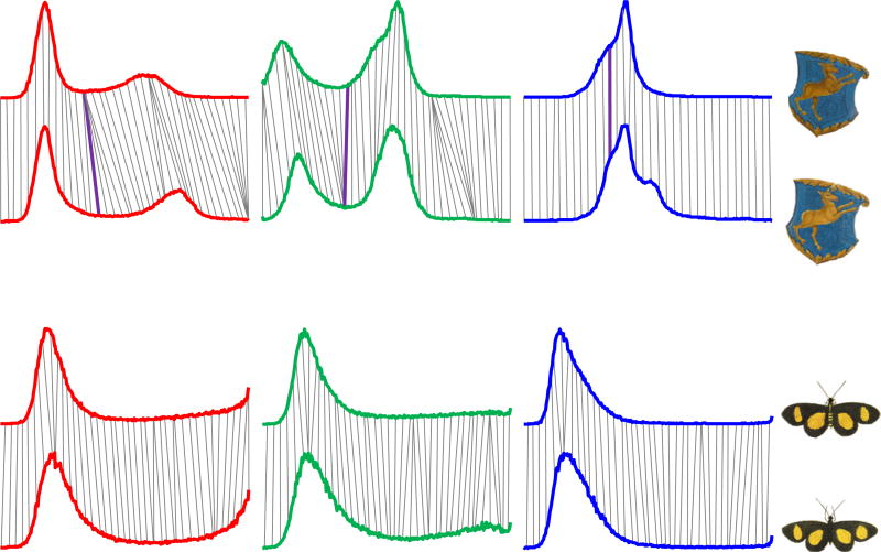
Because color is typically represented in a three dimensional RGB space, it naturally forms a multidimensional time series, as shown The two pairs of examples shown in Fig. 3 are markedly different. In the pair of heraldic shields, each color needs to warp independently. A detailed, high-resolution examination of the images suggests why. While the blue background appears identical in each shield, the gold coloring of the deer is much darker in the uppermost example (this is easier to see in the large format images available at Footnote 1). This difference is probably explained by the fact that the book took four years to produce, and maintaining exact hues over that time period would have been very difficult, especially with 16th century pigment technology.

Fig. 3.

The color histograms of four objects taken from sixteenth century manuscripts. From left to right the red, green and blue channels are presented. Each channel has been independently aligned by DTW. top The two examples from family crest of Lucas Fugger have radically different warpings in each of the three color channels, perhaps reflecting the fact that the book was created over a 4 year period. bottom In contrast, the two butterfly examples have essentially identical alignments (Albertus 1734) (Color figure online)

To make this clearer, we picked a single point just left of center on each channel of the lighter shield and recolored and thickened the hatch line that illustrates the warping. As we can see, in the blue channel the line is vertical, indicating no warping, in the green channel the line leans forward, and in the red channel the line leans backwards. This observation immediately explains the unintuitive clustering shown in Fig. 2 right. By using DTW_D we forced all channels to warp in a single compromised way. If we simply use DTW_I we do obtain the correct clustering here.

This discussion seems to argue in favor of using DTW_I, at least for images. However, there are examples in which all color channels warp in the same way, as in the butterflies in Fig. 3 bottom (see also Fig. 5 of Zhu and Keogh (2010)). This happens if one image is simply sun-faded, or it can be an artifact of the scanning process. In such situations we are better off using DTW_D which finds the best warping by pooling evidence from all three sources of information.

Fig. 5.

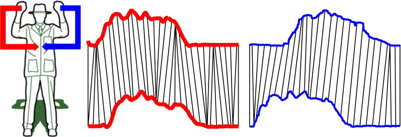
left A cricket umpire signaling “TV-Replay.” right The Dynamic Time Warping distance between two time series of the X-axis from the right and left hand

Our work has two implications for the time series research community: we free researchers/implementers from having to decide which technique to use for their problem; and, because error(DTW_A) will be minimum[error(DTW_D), error(DTW_I)], they can use our method safe in the knowledge that they did not choose the suboptimal method.

However, this greatly understates the case, as the correct inequality implied by our workis the more unintuitive error(DTW_A) ≤ minimum[error(DTW_D), error(DTW_I)]. That is to say, on some datasets our method can be significantly more accurate than either of the rival methods.

2 Definitions and background

We present the definitions of key terms that we use in this work. For our task at hand, each object in the dataset is a time series.

Definition 1

A Time Series T = t₁, t₂, …, t_n is an ordered set of real values. The total number of real values is equal to the length of the time series. A dataset D = {T₁, T₂,…, T_m} is a collection of M such time series.

We are interested in multi-dimensional time series:

Definition 2

Multi-Dimensional Time Series (MDT) consist of M individual time series (M ≥ 2) where each time series has n observations:

$$\begin{array}{l}{Q}_1=q_{1,1},q_{2,1},q_{3,1},\dots q_{\mathrm{n},1}\hfill \\ Q_2=q_{1,2},q_{2,2},q_{3,2},\dots q_{\mathrm{n},2}\hfill \\ \cdots \hfill \\ Q_{\mathrm{M}}=q_{1,\mathrm{M}},q_{2,\mathrm{M}},q_{3,\mathrm{M}},\dots q_{\mathrm{n},\mathrm{M}}\hfill \end{array}$$

If we wish to compare two time series, we could use the ubiquitous Euclidean distance. However, the DTW distance subsumes the Euclidean distance as a special case and has been shown to be significantly more accurate in virtually all domains (Ding et al. 2008; Rakthanmanon et al. 2013). Unlike the Euclidean distance’s strict one-to-one alignment, DTW allows a one-to-many alignment, as illustrated in Fig. 1. To align sequences using DTW, an n-by-n matrix is constructed with the (i, j) element being the squared Euclidean distance d (q_i, c_j) between the points q_i and c_j. A warping path P is a contiguous set of matrix elements defining a mapping between Q and C. The tth element of P is defined as p_t = (i, j)_t, so we have:

$$P=p_1,p_2,\dots ,p_t,\dots ,p_{T}n\le T\le 2n-1$$

The warping path that defines the alignment between the two time series is usually subject to several constraints: the warping path must start and finish in diagonally opposite corner cells of the matrix, the steps in the warping path are restricted to adjacent cells, and the points in the warping path must be monotonically spaced in time. In addition, virtually all practitioners using DTW also constrain the warping path in a global sense by limiting how far it may stay from the diagonal (Ding et al. 2008; Papapetrou et al. 2011). A typical constraint is the Sakoe–Chiba Band which states that the warping path cannot deviate more than R cells from the diagonal (Ding et al. 2008; Papapetrou et al. 2011; Rakthanmanon et al. 2013). This constraint prevents pathological warpings (for example, a single heartbeat mapping to ten heartbeats) and is at the heart of the LB_Keogh lowerbounding technique, which is used in virtually all speedup techniques for DTW (Aach and Church 2001; Ding et al. 2008).

While there are exponentially many warping paths that satisfy the above conditions, we are only interested in the path that minimizes the warping cost:

$$\mathit{\text{DTW}}(Q,C)=\text{min}\left\{\sqrt{\sum _{t=1}^T{p}_t}\right\}$$ (1)

This path can be found using dynamic programming to evaluate the following recurrence, which defines the cumulative distance D(i, j) as the distance d(i, j) found in the current cell and the minimum of the cumulative distances of the adjacent elements (Kruskal and Liberman 1983; Rabiner and Juang 1993):

$$\begin{array}{ll}D(i,j)=\hfill & d(q_i,c_j)+\text{min}\{D(i-1,j-1),D(i-1,j),\hfill \\ \hfill & D(i,j-1)\}\text{in which}:d(q_i,c_j)={(q_i-c_j)}^2\hfill \end{array}$$ (2)

While this recursive function is elegant and can be tersely implemented, in practice the community uses an iterative algorithm, which is faster and amiable to various early abandoning optimizations (Aach and Church 2001; Ding et al. 2008). Moreover, the iterative algorithm implementation only constructs and considers a single column of the matrix at a time and, thus, has a space complexity of just O(n).

The Euclidean distance between two sequences is a special case of DTW, where the tth element of P is constrained such that p_t = (i, j)_t, i = j = t. This review of DTW is necessarily brief; we refer the interested reader to Aach and Church (2001), Ding et al. (2008), Kruskal and Liberman (1983), and Rabiner and Juang (1993) for more details.

2.1 Generalizing to the multi-dimensional case

The DTW distance, as formalized in Eq. 2, is applicable to only single-dimensional time series, leaving open the question of how to extend it to the multi-dimensional time series (MDT) case. Consider both Q and C as two M-dimensional time series; we show two possible approaches for doing this, DTW_I and DTW_D:

Definition 3

DTW_I is the cumulative distances of all dimensions independently measured under DTW. If DTW(Q_m,C_m) is defined as the DTW distance of the mth dimension of Q and the mth dimension of C, we can write DTW_I as:

$${\mathit{\text{DTW}}}_I(Q,C)=\sum _{m=1}^M\mathit{\text{DTW}}(Q_m,C_m)$$ (3)

In Eq. 3, each dimension is considered to be independent, and DTW is allowed the freedom to warp each dimension independently of the others. The case when M is two was shown in Fig. 1b.

We can also compute the multi-dimensional DTW in a manner that forces all dimensions to warp identically, in a single warping matrix. In other words, the independence of dimensions is no longer allowed, and we assume mutual dependence between all dimensions. We define DTW_D as:

Definition 4

DTW_D is calculated in a similar way to DTW for single-dimensional time series (Eq. 2), except that we redefine d(q_i, c_j) as the cumulative squared Euclidean distances of M data points instead of the single data point used in the more familiar one-dimensional case. Formally, if q_{i, m} is the ith data point in the mth dimension of Q and c_{j, m} is the j data point in the mth dimension of C, we replace d(q_i, c_j) in (Eq. 2) with:

$$d(q_i,c_j)=\sum _{m=1}^M{(q_{i,m}-c_{j,m})}^2$$ (4)

To make our distance measure invariant to scale and offset, we need to z-normalize each dimension of the time series before computing their DTW distance. As demonstrated in Keogh and Kasetty (2003), even tiny differences in scale and offset rapidly swamp any similarity in shape. Note that this allows us to meaningfully compute either variant of the multi-dimensional DTW, even if the individual dimensions are not commensurate or are in different units, such as accelerations and rotations.

Using both DTW_D and DTW_I distance measures to classify a time series exemplar, T , four different cases may occur:

1. T gets correctly classified by both DTW_I and DTW_D.

2. T gets misclassified by both DTW_I and DTW_D.

3. T gets classified correctly by DTW_I but misclassified by DTW_D.

4. T gets classified correctly by DTW_D but misclassified by DTW_I.

We are only interested in cases 3 and 4. We call such exemplars iSuccess and dSuccess, respectively:

Definition 5

iSuccess is the set of time series exemplars that are classified correctly under DTW_I but misclassified under DTW_D.

Definition 6

dSuccess is the set of time series exemplars that are classified correctly under DTW_D but misclassified under DTW_I.

Having reviewed the necessary formal definitions, we are now in a position to introduce our observations about the relative merits of DTW_D and DTW_I.

3 Observations

We begin with some informal notation. We say a dataset is “in D” if we expect DTW_D to achieve higher accuracy and “in I” if we anticipate DTW_I will be more accurate. In the introduction we claimed that there are datasets in which we expect DTW_D to outperform DTW_I and vice versa. A natural question to ask is under what conditions we can expect each of these methods to be superior. As we shall see, one of the fundamental contributions of this work is to make this question moot by producing an algorithm that is always at least as good as the better choice. Nevertheless, it is instructive to ask and attempt to answer this question.

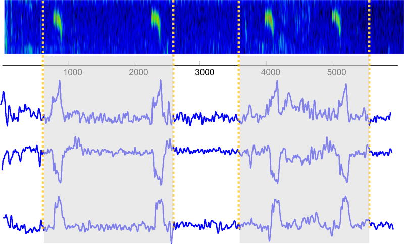
Assume that the data in question corresponds to an event. An event could be an arrhythmic heartbeat, the writing of the letter ‘Z,’ a golf swing, a bird call, a self-driving car parallel parking, etc. Further assume that we have multi-dimensional time series recordings of such events. It is possible that each dimension is simply recording two views of the same physical phenomena. For example, consider the MFCC coefficients of the bird call shown in Fig. 4.

Fig. 4.

Three coefficients from the MFCC space of a Southern Chestnut-Tailed Antbird (Myrmeciza hemimelaena). This bird’s call is typically transcribed as “klee-klee” (Ridgely and Tudor 2009); thus, the above shows two calls, the second being significantly briefer

It is clear that while the coefficients are (somewhat) independent in the Y-axis values they can take on, they are not independent in the time axis. In the second bird call all the relevant peaks and valleys move by exactly the same amount in the time axis. Because of this structure, we strongly expect that this dataset is in D. In contrast, consider the event shown in Fig. 5 of a cricket umpire signaling TV-Replay, in which the umpire traces a rectangle representing a television screen.

Here we have measured a multi-d time series that consists of the X-axis acceleration of sensors worn on each wrist. Note that, in contrast to the bird call example, the two time series are very unlikely to be perfectly dependent in how they evolve in the time axis. Try as he might, the umpire could not move both hands in a perfectly symmetric fashion. There are at least two possible and non-exclusive sources of difference:

• Lag Here, we imagine that the umpire favors his dominant hand, and the other hand follows at a more or less constant speed, but a fraction of a second behind.

• Loose Coupling Here, the event does cause two or more things to happen, both of which are recorded as a time series, but there is more freedom in the performance of the event. For example, if the event is the umpire wishing to signal a Leg-Bye, he will tap his raised knee with this hand. However, while he typically uses his dominant hand to do this, he may touch either knee. Moreover, his “free” hand may rest by his side, or he may raise it, and even waive it slightly, to drawn attention to the fact he is making a signal. This variability in performance means that two wrist-worn sensors are only very loosely coupled for this event.

In the next section, we will explicitly test the effects of these factors with some experiments. To do this we consider a dataset that we are sure is in D, and then we synthetically add increasing amounts of lag and loose coupling to see if this would move the dataset into I .

We consider a handwriting dataset, which we are confident is in D. Because we are considering the X and Y accelerations of the point of the writing tip of a pen, the two dimensions are physically coupled. Here, an event is the production of one of the twenty-six lower-case letters. We estimate the error rate of classification by randomly dividing the 5000 objects into a stratified 1000/4000 train test split thirty times and reporting the average error rate.

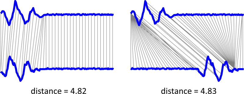
It is critical to note that, in this dataset, if we were considering only the one-dimensional case, our synthetic modifications of the data would make essentially no difference to the distances DTW returns, or the overall error rate. As shown in Fig. 6, even a huge change in the lag makes almost no difference to the single-dimensional DTW case.

Fig. 6.

For the one-dimensional case, adding lag to one of the time series can change the warping drastically, without changing the distance by a significant amount

Thus, all effects shown in thenext two sections are due not to the effects of modifying the data objects per se, but to the effect this has on DTW_D and DTW_I.

3.1 The effect of lag

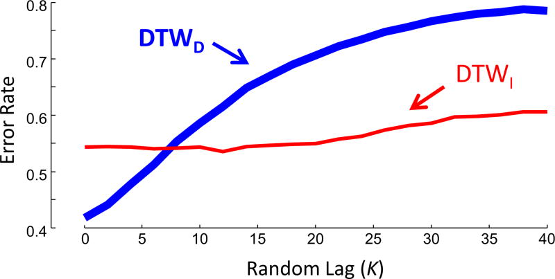
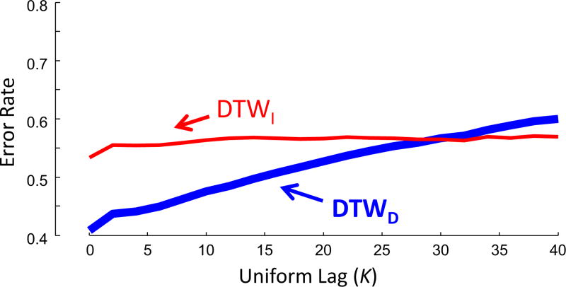
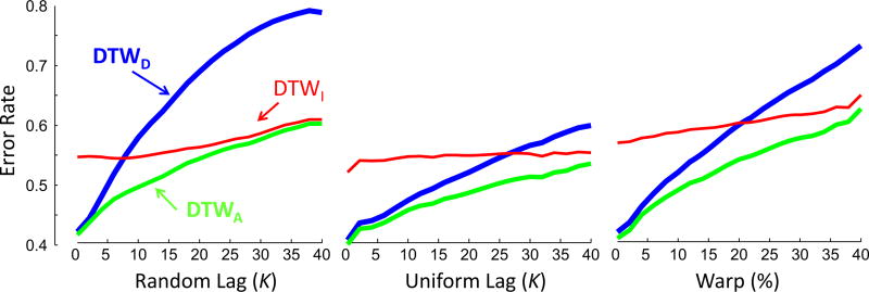
We induce lag in one of two ways. First, for each object we add Random Lag of K by shifting just the Y-axis by an amount randomly chosen from the range [0, K]. Second, we add a Fixed Lag variant by shifting just the Y-axis by increasing values of K. For clarity, in this variant all objects will have the same lag of exactly K. In Fig. 7 we show the effect of varying the amount of Random Lag from zero to forty.

Fig. 7.

The effect of adding Random Lag on the classification accuracy of DTW_D and DTW_I

In Fig. 8 we show the effect of varying the amount of Fixed Lag, again from zero to forty.

Fig. 8.

The effect of adding Fixed Lag on the classification accuracy of DTW_D and DTW_I

If we consider just the values at either end of the range, this provides us with the first experimental evidence that datasets exist that are strongly in D, along with datasets (albeit contrived here) that are strongly in I. More generally, the trend lines in the figure confirm our claim that Lag is one of the elements responsible for datasets falling in D or I. Note that the effects are not small; the wrong choice of DTW_D or DTW_I here can almost double the error rate.

3.2 The effect of loose coupling

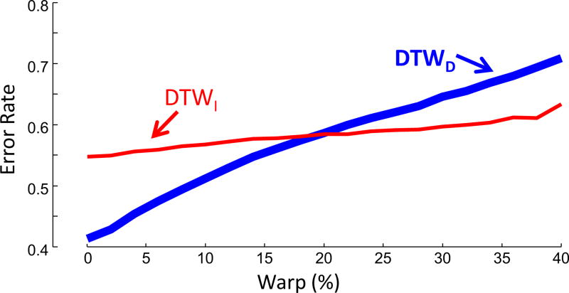
We create synthetic loose coupling by adding increasing amounts of random warping to just the Y-axis of each exemplar. For brevity, and to enhance the flow of the presentation, we relegate the explanation (and the actual code) of how we do this to the supporting website.¹ However, we note that the modified data is plausible and realistic data. For example, if we use it to regenerate the original letters, they are readable and believable as a person’s handwriting. Fig. 9 shows the effect of increasingly loose coupling.

Fig. 9.

The effect of adding Fixed Warping on the classification accuracy of DTW_D and DTW_I

Once again, these results provide us with evidence that some datasets are in D and some are in I, and that loose coupling can be a reason for this division.

3.3 Implication of observations

At first blush we might interpret the above results as implying that all datasets lie on a spectrum between being strongly in D and strongly in I. If true, then the only task left to us is to discover where on the spectrum a dataset falls so that we can use the correct technique.

However, this idea has two difficulties. For some datasets we may not have enough training data to learn whether we are in D or in I with high confidence. The second issue is simply that the assumption that all datasets lie on such a spectrum misses a crucial point. It is possible that the suitability for DTW_D or DTW_I occurs at a class-by-class level, or even an exemplar-by-exemplar level, not at a dataset-by-dataset level.

It is easy to imagine such examples. Suppose we have accelerometers on both wrists of a tennis player, and our classification task is to label data into the following shot types {serve | forehand | lob | other}. For many exemplars we might expect DTW_I to work best, since the hands are generally loosely coupled in tennis. However, for some classes, such as the backhand, most players use a two-handed grip, temporarily coupling the two accelerometers. This would give us a class-by-class-level difference in the suitability of the warping technique. Moreover, some players, notably French professional Jo-Wilfried Tsonga, switch between one-handed and two-handed back-hand shots during the game. This would give us an exemplar-by-exemplar level difference in the suitability of the warping technique.

3.4 Further discussion

The reader may wonder why we need DTW_D at all. It appears that DTW_D is just a special case of DTW_I, and therefore unnecessary. In other words, if both warping paths created by DTW_I happen to be the same, the results are logically equivalent to DTW_D. Since there is nothing preventing this from happening, one might imagine that DTW_D is simply subsumed as a special case of DTW_I, and the results above are an error or anomaly of some kind.

The reason why we need both DTW_d and DTW_I is subtle and underappreciated. When we perform a DTW_I calculation and find it produces a relatively small distance, it may have achieved this with radically different warpings for each axis.

In contrast, DTW_D must use the same warping for both dimensions. Thus, in a sense, the fact that it could achieve a small distance, in spite of the same warping constraint, is extra evidence of similarity.

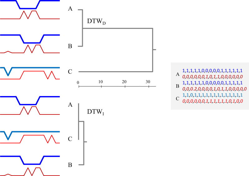
We can illustrate this with the simple experiment shown in Fig. 10. Here we have three 2-dimensional time series. Subjectively we would surely group them {{A,B},C}, as B is created by simply copying A, shifting the “patterns” one place to the right, and adding a tiny “bump” in the 3rd value of B. Nevertheless, if we cluster these objects with DTW_I, we get an extraordinarily unintuitive result, suggesting {{A,C},B}.

Fig. 10.

Three 2-dimensional time series (raw values shown in inset) single-linkage hierarchically clustered using DTW_D (top) and DTW_I (bottom). Here DTW_Dproduces an intuitive clustering, closely linking A and B, whereas DTW_I uses its greater representational flexibility to produce a bizarre result, finding A to be identical to C

This may be easier to appreciate with an analogy. Imagine we have two distance measures, NAME_D and NAME_I, that measure the distance between a target person’s name (say, “Anne Price”) and the set of names we find in a small address book. The underlying measure we assume is a string edit distance. The NAME_I function calculates the most similar first and last names independently, perhaps finding “Anne Smith” and “Bob Price” in the address book to produce a distance of zero. In contrast, the NAME_D function calculates the distances dependently, that is to say, from the same individual. Imagine that NAME_I reports a distance of one, having found a person called ‘Anna Price’. While the latter distance of one is greater than the former distance of zero, we would almost certainly be more impressed by the similarity of the latter.

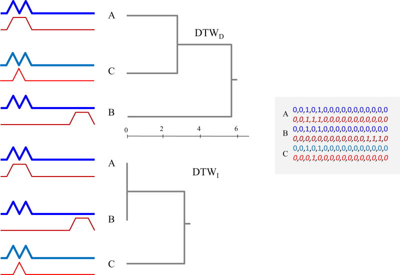
The example illustrated in Fig. 10 shows DTW_D outperforming DTW_I so forcefully that the reader may now wonder why we need DTW_I at all. As previously noted, DTW_D uses the same warping path for all dimensions to measure their distances. Therefore, DTW_D may not be a suitable distance measure for instances with lag, simply because of using only one warping path (recall the three diverse warping paths for each of the color channels shown in Fig. 3 top). For exemplars including lag between dimensions, DTW_I is capable of measuring the distances independently and being invariant to the lag. We illustrate this in Fig. 11.

Fig. 11.

Three 2-dimensional time series (raw values shown in inset) single-linkage hierarchically clustered using DTW_D (top) and DTW_I (bottom). Here DTW_Iproduces an intuitive clustering, closely linking A and B, whereas DTW_D uses only one warping path to measure distances therefore producing a bizarre result, finding A to be identical to C. Compare to Fig. 10

Here instances A and B should belong to the same cluster since both are the same, except B includes a large lag in the second dimension (illustrated in red). As shown in Fig. 11, DTW_D clusters A and C into the same subtree, simply because there is no lag in the second dimension of C. However, DTW_I correctly clusters A and B the same because the lag in the second dimension of B is ignored by DTW_I.

The reader may wonder if our observations are true but irrelevant, as we have only demonstrated our claims for contrived data up to this point. In our experimental section we give compelling evidence on several real-world datasets, but here we give a visually intuitive example. In Fig. 12 we show two dimensions of the telemetry from an oil refinery. In the first day shown, these two time series have near-perfect correlation, suggesting a very tight coupling. However, in the first half of the next day a connecting valve is closed, and the two time series become almost completely uncoupled.

Fig. 12.

Two dimensions from a two-day sequence from the telemetry of a Delayed Coker. In the last 12 h of Day One, the two pressure readings are tightly coupled, but in the first twelve hours of Day Two, they are almost completely uncoupled

More generally, we have made similar observations in many datasets in scientific and medical domains. It seems quite common that the strength and type of relationship (correlation is not quite the right word here) between two time series can ebb and flow over time, and neither DTW_I nor DTW_I is always best.

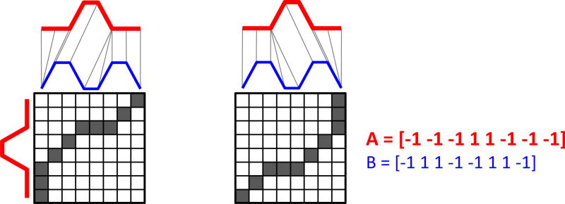
Finally, before continuing, we must discount a solution that may have occurred to the reader, perhaps based on visual inspection of Fig. 1. One might imagine that a large dissimilarity between the warping paths in DTW_I could indicate that the exemplar comparison in question is best suited to DTW_I. However, this is not the case. In general, it is possible that two warping paths could be arbitrarily different, but reflect identical DTW distances. In Fig. 13 we illustrate this with a toy example. While this example uses symmetric data to elucidate our point, this observation is more generally true.

Fig. 13.

An example of two warping paths that are very different, but reflect identical DTW distances of 2.80

4 Proposed framework

In essence, our task reduces to a meta-classification problem. Given an instance to classify, we must first decide whether it is “an object best classified by DTW_I” or “an object best classified by DTW_D.” More formally:

Problem Statement Given that we are using NN-DTW to classify an exemplar Q, and that we have discovered the nearest neighbor to Q under both DTW_I and DTW_D, if the classes of the two nearest neighbors differ, predict the distance function most likely to be correct.

Our problem statement is superficially similar to a “gating network” in a Mixture of Experts (ME), a technique frequently used in neural networks and some other classifiers (Yuksel et al. 2012). Using the divide and conquer principle, several “experts” that are either regression functions or classifiers are created such that they specialize in a particular region of the input space. The gating network defines those regions where the individual expert opinions are trustworthy, and uses a probabilistic model to combine the expert’s opinions.

There are many variants of ME (see Yuksel et al. (2012) and references therein). However, in contrast to most versions, we have a much narrower task. We have exactly two experts, and we are “weighting” their opinions only in a strictly binary sense.

We propose the following solution to our problem. Offline, on the training data, we will compute a threshold. At query time, we will compute a score S, and choose which method to trust based on the value of S relative to the threshold. In order to best explain our framework, we first explain how our classification model works, given that a threshold has been learned from the trainData. Later, in Sect. 4.2, we consider the task of learning the threshold. If we have a lack of labeled data, we outline two possible approaches. We can either learn the threshold from a different dataset, from the same or similar domain, or we can simply hardcode the threshold to one, which gives us much of the benefit of our observation. We have explored both ideas in Footnote 1.

4.1 Adaptive classifier for MDT

Table 1 outlines our classification algorithm. In line 1 the algorithm finds the nearest neighbor distance in the training set for Q under DTW_D, minD. In line 2 we find the nearest neighbor distance under DTW_I, minI. In line 3 the procedure divides minD by minI, which is our scoring function, S. In lines 4 to 8 the algorithm compares our scoring function, S, to the previously learned threshold. If S is greater than the threshold, we believe that Q is most likely in I and thus return DTW_I as the distance measure for classification, whereas if S is less than or equal to the threshold, we predict that Q is most likely in D, and the function returns DTW_D.

Table 1.

Adaptive classification algorithm

Procedure adaptive_Classifier (Q, trainData, threshold)
Input: A time series query, Q, the labeled data, trainData, a threshold;
Output: An adaptive distance measure to classify Q, DTWA ;
1	minD ← Nearest_Neighbor_Distance_D (Q, trainData);
2	minI ← Nearest_Neighbor_Distance_I (Q, trainData);
3	S ← minD / minI;
4	if S > threshold
5	DTWA ← DTWI ;
6	else
7	DTWA ← DTWD ;
8	end if
9	Return DTWA

We formally define our scoring function as:

$$S=\frac{{\mathit{\text{Nearest Neighbor Distance under DTW}}}_D}{{\mathit{\text{Nearest Neighbor Distance under DTW}}}_I+\in }$$ (5)

The epsilon in the denominator is to prevent division by zero, a value that is theoretically possibility but never observed. While S can change in the range of [ε, ∞], in practice we find its value to always be in the range of [0.5, 2].

Having explained our simple classification algorithm, all that remains is to explain how we set the threshold (and why). In fact, hardcoding the threshold to a value of exactly one works very well and allows the algorithm in Table 1 to beat the rival methods. However, we can further improve the accuracy by tuning the threshold, so in the next section we will explain how that is done.

4.2 Learning the adjusted threshold

In order to learn the threshold we use in Table 1, we first need to identify the iSuccess (def. 5) and dSuccess (def. 6) exemplars in the training set using cross validation (Table 3). As shown in Table 2, we consider four cases based on whether iSuccess and dSuccess are empty sets or not.

Table 3.

An algorithm to find iSuccess and dSuccess and compute S scores for all their exemplars

Procedure find_Scores (trainData)
Input: Labeled data, trainData;
Output: S scores for iSuccess and dSuccess, S_iSuccess and S_dSuccess;
1	for n ← 1 to size(trainData)
2	minD ← Nearest_Neighbor_Distance_D (trainData(n), trainData);
3	minI ← Nearest_Neighbor_Distance_I (trainData(n), trainData);
4	if (trainData(n).label == Nearest_Neighbor_D ().label &&
5	trainData(n).label != Nearest_Neighbor_I ().label )
6	S_dSuccess.add (minD / minI);
7	end if
8	if (trainData(n).label != Nearest_Neighbor_D ().label &&
9	trainData(n).label == Nearest_Neighbor_I ().label )
10	S_iSuccess.add (minD / minI);
11	end if
12	end for

Table 2.

Learning the adjusted threshold

Procedure Learn_Threshold (trainData)
Input: Labeled data, trainData;
Output: Adjusted threshold, threshold;
1	[S_iSuccess, S_dSuccess] ←find_Scores (trainData);
2	if (S_iSuccess == ϕ && S_dSuccess ==ϕ)
3	threshold ← 1;
4	else if (S_iSuccess ==ϕ&& S_dSuccess != ϕ)
5	threshold ← max(S_dSuccess) ;
6	else if (S_iSuccess !=ϕ && S_dSuccess == ϕ)
7	threshold ← min(S_ iSuccess) ;
8	else if (S_iSuccess! = ϕ && S_dSuccess != ϕ)
9	threshold ← Decision_Tree (S_iSuccess, S_dSuccess);
10	end if

In line 1 we run the subroutine in Table 3 to find all the S scores for iSuccess and dSuccess, and then we consider four cases on the two sets. Line 2 is the case in which both sets are empty, so the problem (at least the training data) is independent of D or I, and picking either DTW_I or DTW_D will make no difference in classifying the data. Therefore, we assign the value one, an arbitrary number, to the threshold in line 3. We note that this case is possible, but we never observed it.

In line 4 we test to see if S_i Success is empty and S_dSuccess is non-empty. If so, the dataset is almost certainly in D, and we need to set the threshold such that the S score for all dSuccess exemplars will be less than the threshold. Therefore, in line 5 the threshold gets assigned to the maximum value of S_dSuccess.

The opposite case, in which S_dSuccess is empty and S_iSuccess is non-empty (line 6), offers evidence that the dataset is in I , and we need to set the threshold such that the S score for all iSuccess exemplars will be greater than the threshold. We ensure this (in line 7) by assigning the threshold to the minimum value of S_iSuccess.

In practice, the three cases above are rare, and in lines 8 to 10 we find the threshold for the most common case in which both S_iSuccess and S_dSuccess are non-empty sets. The best threshold is a value that maximizes the total number of S_iSuccess with values greater than the threshold and S_dSuccess with values less than the threshold. Finding such a threshold is essentially the decision tree problem of maximizing the information gain by finding the optimal split point. For more details on information gain, we refer the interested reader to Ye and Keogh (2009) and Quinlan (1986).

Recall the function find_Scores (trainData) called in Table 2. The function uses cross validation to find the two sets, iSuccess and dSuccess, then calculates the S scores (Eq. 5) for all their exemplars. The algorithm is described in Table 3. In line 1 we apply cross validation to the entire trainData. In line 2 we calculate the nearest neighbor distance under DTW_D for each exemplar, and in line 3 we do the same under DTW_I. In lines 4 to 7, if the exemplar in the trainData is classified correctly under DTW_D and misclassified under DTW_I, the S score (Eq. 5) is calculated and gets added to S_dSuccess. In line 8 to 11, if the exemplar is misclassified under DTW_D and classified correctly under DTW_I, we calculate the S score and add it to S_iSuccess.

4.3 The intuition behind our scoring function, S

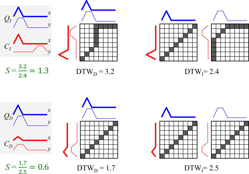
In this section we explain the intuition behind our scoring function (Eq. 5), introduced in Sect. 4.1. We will show how the ratio of the nearest neighbor distance under DTW_D (minD) and DTW_I (minI) is capable of discriminating multi-dimensional time series in I from exemplars in D. For any time series in I, each dimension is at least somewhat independent; therefore, exemplars that are from the same class and are warped/shifted independently in each dimension exist in the training set. Figure 14 top shows a time series in I, Q _I and its nearest neighbor in the training set, C_I.

Fig. 14.

top Computing the S score for a two-dimensional time series in I. bottom S score calculation of a two-dimensional time series in D

Note that in our proposed algorithm in Sect. 4.1 the nearest neighbors under DTW_I and DTW_D are not necessarily the same; however, for simplicity of presentation we consider C_I as the nearest neighbor under both DTW_I and DTW_D. Since Q_I is in I and its dimensions are warped independently, the DTW_I distance will be less than or equal to the DTW_D simply because DTW_I is allowed the freedom to find the nearest distance independently in each dimension. In Fig. 14 top, DTW_I calculates the distance in two different paths, whereas DTW_D has only one path to pick which is a combination of the two paths in DTW_I and eventually produces a larger distance. For any instance in I, minD is larger and minI gets smaller; therefore, minD/minI tends to be larger.

In Fig. 14 bottom we show an instance, Q_D, which is in D. In this case the nearest neighbor in the training set, C_D, will be an exemplar in which both dimensions are dependently warped. In such a case, the warping path for both dimensions in DTW_I are the same as, and similar to, the path in DTW_D. In contrast to the previous case, DTW_I does not take advantage of different warping paths in order to achieve a lower distance score compared to DTW_D. However, we show for the same warping path, the distance under DTW_I is larger than the DTW_D distance. Since DTW_D and DTW_I both take the same path, we can compare their cumulative distances in a meaningful way.

If q_{i, m} is the ith data point in the mth dimension of Q_D and c_{j, m} is the jth data point in the mth dimension of C_D, for the two-dimensional case in Fig. 14 bottom, we can show the following:

$$\begin{array}{l}{\mathit{\text{DTW}}}_D(Q_D,C_D)\hfill \\ =\sqrt{{\sum }_{i,j=1}^n[{(q_{i,1}-c_{j,1})}^2+{(q_{i,2}-c_{j,2})}^2]}\hfill \\ <\sqrt{{\sum }_{i,j=1}^n[{(q_{i,1}-c_{j,1})}^2+{(q_{i,2}-c_{j,2})}^2+2(q_{i,1}-c_{j,1}\left)\right(q_{i,2}-c_{j,2}\left)\right]}\hfill \\ =\sqrt{{\sum }_{i,j=1}^n{\left[\right(q_{i,1}-c_{j,1})+(q_{i,2}-c_{j,2}\left)\right]}^2}\hfill \\ ={\sum }_{i,j=1}^n\left[\right(q_{i,1}-c_{j,1})+(q_{i,2}-c_{j,2}\left)\right]\hfill \\ ={\sum }_{i,j=1}^n\left[\right(q_{i,1}-c_{j,1}\left)\right]+{\sum }_{i,j=1}^n\left[\right(q_{i,2}-c_{j,2}\left)\right]\hfill \\ =\sqrt{{\sum }_{i,j=1}^n{(q_{i,1}-c_{j,1})}^2}+\sqrt{{\sum }_{i,j=1}^n{(q_{i,2}-c_{j,2})}^2}\hfill \\ ={\mathit{\text{DTW}}}_I(Q_D,C_D)\hfill \end{array}$$

Accordingly, for a time series in D, minD is smaller and minI gets larger; therefore, minD/minI tends to be smaller. We considered a two-dimensional time series here and assumed that for a query in I, the path in DTW_I and DTW_D are exactly the same; however, we can simply generalize the above illustration to dimensions greater than two, and for queries in I, different but similar paths for both DTW_I and DTW_D.

We have shown that our scoring function, S (cf. Eq. 5), tends to produce larger values for queries in I and smaller values for queries in D, as illustrated above; thus, our scoring function is capable of discriminating time series in I from exemplars in D. We will demonstrate the effectiveness of our scoring function with extensive experiments in the next section.

5 Experiments

We have designed all our experiments to ensure that they are very easy to reproduce. A supporting webpage (see Footnote 1) contains all the code, datasets, and raw data spreadsheets used in this work. Moreover, although this work is completely self-contained, the webpage contains additional experiments for the interested reader.

In addition to comparing to DTW_D and DTW_I, we also compare to the classification using each individual dimension, which we refer to using the notation DTW(_1st), DTW(₂nd), etc.

It is important to note that all experiments use exactly the same base algorithm, one nearest neighbor, and exactly the same train/test splits. Thus, any differences in results can be attributed solely to the distance measure used.

It is known that the warping window width can slightly affect the classification accuracy. As this issue is orthogonal to our work, we simply set the warping window constraint for DTW to be 20% for all experiments (Ding et al. 2008).

5.1 Recognition of cricket umpire signals

Cricket is a very popular game in British Commonwealth countries. The game requires an umpire to signal different events in the game to a distant scorer/bookkeeper. The signals are communicated with motions of the hands. For example, No-Ball is signaled by touching each shoulder with the opposite hand, and TV-Replay, a request for an off-field review of the video of a play, is signaled by miming the outline of a TV screen (cf. Fig. 5). A complete dictionary of signals can be found in Footnote 1.

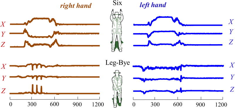
The dataset introduced in Ko et al. (2005) consists of four umpires performing twelve signals, each with ten repetitions. The data, recorded at a frequency of 184Hz, was collected by placing accelerometers on the wrists of the umpires. Each accelerom-eter has three synchronous measures for three axes (X, Y and Z). Thus, we have a six-dimensional MDT from the two accelerometers and we can combine any number of them to create a multi-dimensional classification problem. Figure 15 shows the data for two example signals, Six and Leg-Bye. To signal Six, the umpire raises both hands above his head. Leg-Bye is signaled with a hand touching the umpire’s raised knee three times.

Fig. 15.

X, Y and Z acceleration data from the right hand (left), a representation of the umpire’s body position (center), and the X, Y and Z acceleration data from the left hand, for the two umpire signals Six and Leg-Bye

We used 40% of the data for training and use the rest as testing data. The classification results using various combinations of dimensions are shown in Table 4.

Table 4.

Classification error rates on the cricket data

Data	DTW(1st)	DTW(2nd)	DTWI	DTWD	DTWA
Xright _Xleft	0.26	0.27	0.13	0.20	0.11
Yright _Xleft	0.17	0.27	0.07	0.04	0.03
Xright _Yleft	0.26	0.14	0.07	0.10	0.06
Yright _Yleft	0.17	0.14	0.04	0.03	0.03
Zright _Zleft	0.18	0.18	0.07	0.06	0.04
Zright _Xleft	0.18	0.27	0.07	0.04	0.04

Note that all combinations support our original claims that neither DTW_D nor DTW_Idominates the other, and that on all datasets, DTW_A is at least as accurate as the better of DTW_D and DTW_I, and often more accurate.

Above we considered only pairs of dimensions, however, the results generalize for any-sized subsets of dimensions. Obviously, adding more dimensions does not guarantee improved accuracy. In Hu et al. (2013) the authors outline a strategy for choosing which dimensions to add to an MDT. Note, however, that this issue is completely orthogonal to our contributions; Table 4 suggests that whatever set of dimensions you choose, you are better off with DTW_A than any other method.

5.2 Accelerometer-based gesture recognition

There is increasing interest in using gesture commands for interacting with and controlling external devices. The results in Kela et al. (2006) suggest that different people often have different interpretations of even simple gestures, and thus it is necessary to learn personalized classifiers on an individual basis.

A widely used benchmark dataset, introduced in Liu et al. (2009), consists of the performances of the gestures shown in Fig. 16 by eight participants. To produce realistic variability in performance, the data was collected on multiple days over three weeks. On each day the participant held a Nintendo Wii remote and repeated each of the eight gestures ten times.

Fig. 16.

Gesture vocabulary adopted from Kela et al. (2006). The dot denotes the start and the arrow the end of the gesture

The dataset consists of 4480 gestures in total: 560 for each participant. The accelerometer has three axes (X, Y and Z); thus, we have a three-dimensional MDT form, and we can combine them to create a two or three multi-dimensional classification problem. We combined every pair of dimensions to create all possible two-dimensional time series and combined all three for the three-dimensional case. The classification results are shown in Table 5.

Table 5.

Error rates for gesture recognition

Data	DTW(1st)	DTW(2nd)	DTW(3rd)	DTWI	DTWD	DTWA
X_Y	0.34	0.48	–	0.23	0.18	0.18
X_Z	0.34	0.41	–	0.13	0.13	0.12
Y_Z	0.48	0.41	–	0.26	0.24	0.23
X_Y_Z	0.34	0.48	0.41	0.11	0.09	0.08

As before, the results support our claim that DTW_A is at least as accurate as the better of DTW_D or DTW_I.

5.3 Word recognition from articulatory movement data

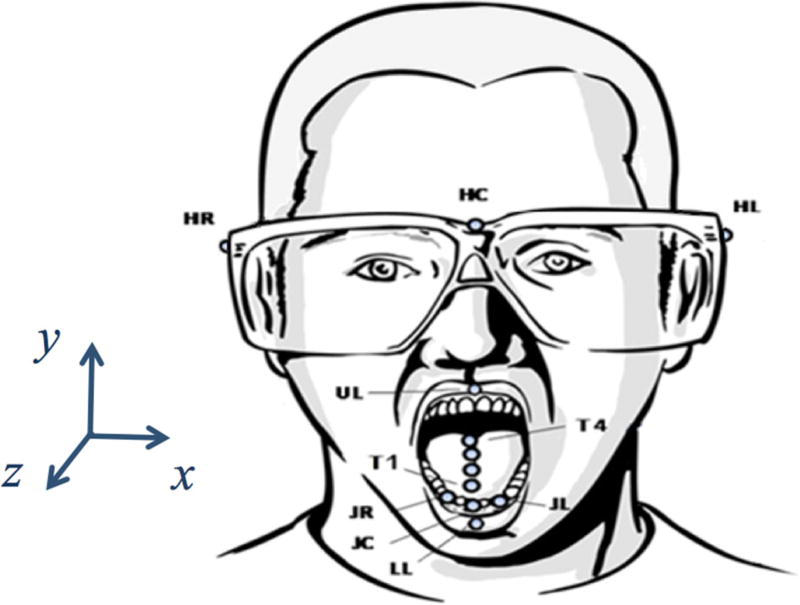
Silent “speech” recognition may potentially facilitate oral communication in people with severe voice impairments, for example, after laryngectomy, a surgical removal of larynx due to the treatment of cancer (Wang et al. 2012, 2013, 2014). Silent speech recognition is to recognize words or sentences from non-audio data (e.g., tongue and lip movement data) (Wang et al. 2014). An Electromagnetic Articulograph (EMA) (Yunusova et al. 2009) is an apparatus used to measure the movement of the tongue and lips during speech. The motion tracking using EMA is registered by attaching small sensors on the surface of the articulators (e.g., tongue and lips). The spatial accuracy of motion tracking using EMA AG500 is 0.5 mm (Yunusova et al. 2009). We consider the EMA dataset in Wang et al. (2013) which contains data collected from multiple native English native speakers producing 25 words. Twelve sensors were used in data collection, each providing X, Y and Z time-series positions with a sampling rate of 200 Hz. As shown in Fig. 17 the sensors are located on the forehead, tongue; from tip to back in the midline, lips and jaw. The three head sensors (Head Center, Head Right, and Head Left) attached on a pair of glasses were used to calculate head-independent movement of other sensors. Tongue sensors were named T1, T2, T3, and T4, from tip to back. For more details about the data collection procedure and description, please refer to Wang et al. (2013).

Fig. 17.

The coordinate system and sensor locations on a participant’s forehead, tongue, lips, and jaw in data collection using EMA. Labels are described in text

Of the total of 36 available dimensions, for brevity and simplicity, we show only some random combinations of dimensions extracted from the sensors on the tongue tip (T1), the upper lip (UL) and lower lip (LL). The classification results are shown in Table 6.

Table 6.

Classification error rates on the continuous articulatory movement dataset

Data	DTW(1st)	DTW(2nd)	DTW(3rd)	DTWI	DTWD	DTWA
T1Z_ULX	0.34	0.59	–	0.25	0.31	0.25
T1Y_ULY	0.38	0.55	–	0.22	0.15	0.13
T1Z_LLZ	0.34	0.47	–	0.17	0.10	0.10
T1Z_LLY	0.34	0.48	–	0.20	0.12	0.11
T1Y_LLY	0.38	0.48	–	0.21	0.14	0.14
T1Y_T1Z	0.38	0.34	–	0.24	0.15	0.15
T1X_T1Y_T1Z	0.32	0.38	0.34	0.15	0.10	0.10
T1X_T1Y_ULY	0.32	0.38	0.55	0.16	0.18	0.14
T1Y_T1Z_LLX	0.38	0.34	0.67	0.12	0.08	0.08
T1Z_LLX_LLY	0.34	0.67	0.48	0.14	0.12	0.10

Yet again, the results support our claim that DTW_A is at least as accurate as the better of DTW_D or DTW_I.

5.4 Revisiting the semi-synthetic data

We reconsider the handwriting data set used in Sect. 3. Recall that the data is real, but manipulated in ways such that it changed from being in D to being in I. In Fig. 18 we revisit these problems, this time using DTW_A. Once again these experiments offer strong support for our claims about DTW_A dominating DTW_I and DTW_D.

Fig. 18.

The experiments shown in Figs. 7, 8 and 9, revisited using the DTW_A technique

5.5 Human activity recognition using smart watches

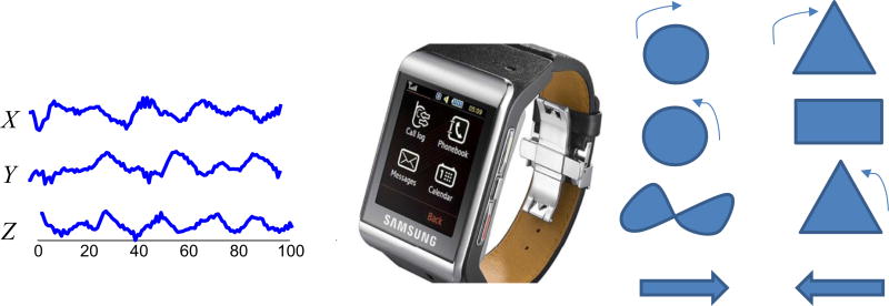
Providing accurate and exploitable information on human activity has become an active field in pervasive computing (Ding et al. 2008; Lara and Labrador 2013). Activity recognition using a smart watch has the potential to be highly useful in modern healthcare by monitoring the patients’ activities and automatically reporting summaries to healthcare providers (Rawassizadeh et al. 2014). In order to detect a specific set of gestures or behaviors during daily activities we can simply use a rejection threshold, which classifies the target gestures from (the much larger space of) non-target activities (Hu et al. 2013). However, in order to detect such gestures/behaviors we need to know the best distance measure to classify the gestures. For this purpose we designed a simple experiment. We asked two users to wear a Samsung Gear 2 and execute 100 performances of eight different gestures. We collected the accelerometer data (X, Y and Z) with a sampling rate of 50 Hz. The eight gestures performed by users and a sample accelerometer data is shown in Fig. 19.

Fig. 19.

left Sample accelerometer data (X, Y and Z) of a gesture. middle A Samsung Gear 2 used to collect activity data. right the eight different gestures considered in our experiments

We combined every pair of dimensions to create all possible two-dimensional time series and combined all three for the three-dimensional case. The classification results are shown in Table 7.

Table 7.

Error rates for activity detection using a smart watch

Data	DTW(1st)	DTW(2nd)	DTW(3rd)	DTWI	DTWD	DTWA
X_Y	0.43	0.46	–	0.25	0.17	0.15
X_Z	0.43	0.50	–	0.28	0.15	0.12
Y_Z	0.46	0.50	–	0.33	0.15	0.15
X_Y_Z	0.43	0.46	0.50	0.22	0.12	0.12

As with previous experiments, the results support our claim that DTW_A is at least as accurate as the better of DTW_D or DTW_I.

5.6 Learning the threshold with sparse training data

The reader may wonder if it is possible to learn the threshold if we have little labeled data to work with. For example, this is a common situation when beginning to use a new gesture-based system (the so-called “cold start” problem).

As noted in Sect. 4.1 in our paper, simply hardcoding the threshold to a value of one gives us much of the benefit of our observation. However, tuning the threshold does help, and we want to obtain the best possible accuracy.

Without claiming to have completely solved this problem, we outline one possible approach here. Our idea is that we can learn the threshold from a different dataset from the same or similar domain. In essence this is a simple form of transfer learning.

For example, if a company releases a smartwatch with gesture recognition capabilities, a good “universal” threshold could be learned and set at the factory. This would allow the system to work well “out-of-the-box,” and possibly be refined and personalized over time.

We have conducted an experiment to demonstrate this idea. For the Gesture Recognition dataset in Sect. 5.2 in our paper, we combined all three dimensions of X, Y and Z from the accelerometer and created two completely disjointed datasets, G₁ and G₂. We learned the threshold from G₁ and used the same threshold to classify G₂. The results are shown in Table 8.

Table 8.

The first and second row correspond to results for classifying G₂ with the threshold learned from G₂ and G₁, respectively

Data	DTW(1st)	DTW(2nd)	DTW(3rd)	DTWI	DTWD	DTWA
X_Y_Z(1)	0.30	0.45	0.37	0.08	0.06	0.05
X_Y_Z(2)	0.30	0.45	0.37	0.08	0.06	0.06

The results tentatively suggest that by adopting the threshold value from a different dataset in the same domain, we can achieve approximately the same accuracy we would have achieved by learning the threshold from a (large sample) of the native dataset.

5.7 What causes a time series to be in D or I?

For all of the experiments considered above, the data sets included a mixture of exemplars in I and D. If this was not true, DTW_A could not have had a lower error-rate. However, an interesting question we have glossed over thus far is what causes an individual time series exemplar to be in D or I? Is it an intrinsic property of the individual exemplar itself or a property of the exemplar in relation to a particular data set? We conducted a wide-ranging investigation of the exemplars’ characteristics in various domains to see if any feature(s) stands out as a discriminator of time series in I vs. in D. We considered the correlation, complexity, Euclidean distance, Minimum Description Length, etc. of dimensions and did not find any useful discriminator.

We have designed a simple experiment which strongly suggests (at least for the data set considered) that the existence of exemplars in I or D strongly depends on the entire data set. A time series, which is in I, may later be in D if we use a different training set for classifying that item. In addition, just the size of the training set can have a significant impact on whether exemplars fall in I or D.

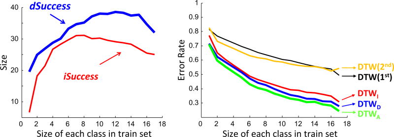
Once again we revisit the handwriting data set we used in Sect. 3. In all iterations we randomly sample ten exemplars from each of twenty-six classes as the test set (a total of 260 items). In the first iteration we randomly pick only a single instance for each class and define it as the train set. Then we classify the test set using DTW_D and DTW_I separately and also count the number of items in iSuccess and dSuccess (cf. Definitions 5 and 6). In the second iteration we randomly pick two instances for each class as the train set and repeat the same steps. We continue the iterations until we reach seventeen exemplars per class. The results are shown in Fig. 20.

Fig. 20.

left The number of elements in iSuccess and dSuccess for train sets of different sizes. right The effect of data set size on accuracy of classification

We believe we can interpret Fig. 20 as follows. First (and only incidentally here), Fig. 20 right supports our claim that DTW_A is at least as accurate as the better of DTW_D or DTW_I, as the green curve for DTW_A dominates all the other approaches for the entire range of training data sizes. Note that all five approaches have almost the same (very high) error-rate when the training set is very small. This is simply because there is very little space for them to differ. In the limit, had we started one value to the left, with zero data, all approaches would have had the exact same error-rate, the default rate.

As the training dataset gets larger, all approaches benefit, just as we expect. However, DTW_A benefits the most. This is because as the training dataset gets larger, there is a greater possibility that some objects to be classified can benefit from choosing the more suitable of the two multi-dimensional variants of DTW. To see this more clearly, in Fig. 20 left we measured the number of objects in iSuccess and dSuccess for the experiments shown in Fig. 20 right. We see that for small train sets the number of items in iSuccess and dSuccess are low. However, when the size of the train set increases, the number of instances in iSuccess or dSuccess begins to increase in spite of the fact that the size of the test sets remains constant.

There is one observation in Fig. 20 left that we have to explain. After some point, the number of items in iSuccess and dSuccess begins to decrease. Why is this? The reason is that, for large enough training sets, there is a greater chance that the nearest neighbor, under both DTW_I and DTW_D, will be the same (true) class. This will make our DTW_A unnecessary (but not harmful to accuracy). A similar effect has been shown for the error-rates of (one dimensional) DTW versus ED classifiers (See Fig. 1 of Shieh and Keogh (2009)). For small datasets, DTW and ED often make different decisions about which item is the nearest neighbor, but as the datasets get larger they tend to agree more and more often, eventually converging to the same error-rate (Shieh and Keogh 2009; Ratanamahatana and Keogh 2004).

In a sense, these observations seem to cast limits on the utility of our proposed ideas. DTW_A will be no better (but critically, no worse) in the case that the training dataset is pathologically small or is arbitrarily large. However, the situation in between is clearly the most common. For example, in virtually all gesture recognition systems it is assumed that the user is willing to provide at least five to ten examples of a gesture so that we can estimate variability of performance (Kela et al. 2006; Liu et al. 2009; Gillian et al. 2011; Ten Holt et al. 2007; Aach and Church 2001; Tang and Dannenberg 2014). But, clearly, we do not expect an individual user to provide one thousand labeled examples of a gesture.

6 Related work

We have deferred a discussion of related work until now when the reader can appreciate the nature of our contributions. While there are hundreds of research efforts that use DTW in a multi-dimensional setting (Ridgely and Tudor 2009; Kela et al. 2006; Ko et al. 2005; Liu et al. 2009; Petitjean et al. 2012; Wang et al. 2013), we are not aware of any work that discusses the relative merits of DTW_I and DTW_D, or even explicitly notes that they are alternatives. The vast majority of researchers seem to think that it makes no difference which method is used, as evidenced by the fact that they usually do not bother to explicitly tell the reader (Liu et al. 2009; Aach and Church 2001; Kale et al. 2012; Tang and Dannenberg 2014). In paper (Liu et al. 2009) they define DTW as a dynamic programming algorithm, which calculates the matching cost and finds the corresponding shortest path. However, it is not clear how they generalize it to the multidimensional case. A handful of papers do mention that there exist two ways of computing dynamic time warping in multi-dimensional time series. For example, the authors in Petitjean et al. (2012) choose DTW_D for classifying satellite images because they argue that satellite images have dependent dimensions in their time series. Other papers, such as Gillian et al. (2011), Aach and Church (2001), and de Mello and Gondra (2008), use DTW_D without pointing out the alternative approach of DTW_I. The authors in Ten Holt et al. (2007), Bashir and Kempf (2008), and McGlynn and Madden (2011) use other methods similar to DTW_I such as adding up all dimensions and dealing with a single dimension time series. For instance, Bashir and Kempf (2008) applies DTW to the data obtained from the sum of all channels in different dimensions. The authors in Ten Holt et al. (2007) normalize and smooth each dimension and then use the total difference among dimensions to find the best synchronization with the regular DTW algorithm.

The ubiquity of multi-dimensional time series, especially given the recent explosion of interest in wearable devices, has produced significant research in speeding up DTW (Rakthanmanon et al. 2013), choosing which subset of dimensions to use (Hu et al. 2013), choosing a setting for the warping window constraint (Ding et al. 2008), etc. However, all such work is orthogonal to (and compatible with) our contributions. We have created an annotated bibliography of which papers use DTW_I vs. DTW_D (Footnote 1).

As we noted above, there is significant research in “gating networks” and related techniques for choosing which classifier to use on a given region of the input space (Yuksel et al. 2012). However, to the best of our knowledge, these ideas have never been applied to time series and are only superficially related to the task at hand.

7 Conclusions

In this work we demonstrate for the first time that of the two obvious ways to do multi-dimensional NN-DTW classification, neither is always superior. We show that the differences are not trivial, as the wrong choice can double the error rate. We introduce a simple algorithm that can pick the method that is most likely to predict the correct class on a case-by-case basis. Our algorithm is simple to implement, and its overhead is inconsequential in terms of both time and space.

For concreteness we have confined our remarks and empirical demonstrations to classification problems, but note that distance measures are at the heart of many time series data mining tasks, including clustering, summarization, motif discovery (Hao et al. 2013), rule mining (Shokoohi-Yekta et al. 2015; Shokoohi-Yekta 2015), and many forms of anomaly detection. In future work we will expand our consideration of our ideas to these tasks.

Finally, in this work we have focused on intuitively explaining our observations/ideas and showing strong empirical evidence for them. However, we plan to revisit our work with a more theoretical framework and prove several useful properties of DTW_A.

References

- Aach J, Church GM. Aligning gene expression time series with time warping algorithms. Bioinformatics. 2001;17(6):495–508. doi: 10.1093/bioinformatics/17.6.495. [DOI] [PubMed] [Google Scholar]
- Akl A, Valaee S. Accelerometer-based gesture recognition via dynamic-time warping, affinity propagation, & compressive sensing. Proceedings of the IEEE international conference on acoustics speech and signal processing (ICASSP); 2010. pp. 2270–2273. [Google Scholar]
- Albertus S. Locupletissimi rerum naturalium thesauri accurata descriptio, et iconibus artificiosissimis expressio, per universam physices historiam: Opus, cui, in hoc rerum genere, nullum par exstitit 1734 [Google Scholar]
- Al-Jawad A, Adame MR, Romanovas M, Hobert M, Maetzler W, Traechtler M, Moeller K, Manoli Y. Using multi-dimensional dynamic time warping for tug test instrumentation with inertial sensors. Proceedings of the IEEE conference on multisensor fusion and integration for intelligent systems (MFI); 2012. pp. 212–218. [Google Scholar]
- Assent I, Wichterich M, Krieger R, Kremer H, Seidl T. Anticipatory DTW for efficient similarity search in time series databases. Proc VLDB Endow. 2009;2(1):826–837. [Google Scholar]
- Bashir M, Kempf J. Reduced dynamic time warping for handwriting recognition based on multidimensional time series of a novel pen device. Int J Intell Syst Technol WASET. 2008;3(4):194. [Google Scholar]
- Das Ehrenbuch der Fugger (The secret book of honour of the Fugger) -BSB Cgm 9460. Augsburg, ca: pp. 1545–1548. mit Nachträgen aus späterer Zeit. [Google Scholar]
- de Mello RF, Gondra I. Multi-dimensional dynamic time warping for image texture similarity. Advances in Artificial Intelligence-SBIA Springer; Berlin: 2008. pp. 23–32. [Google Scholar]
- Ding H, Trajcevski G, Scheuermann P, Wang X, Keogh E. Querying and mining of time series data: experimental comparison of representations and distance measures. Proc VLDB Endow. 2008;1(2):1542–1552. [Google Scholar]
- Ermes M, Parkka J, Mantyjarvi J, Korhonen I. Detection of daily activities and sports with wearable sensors in controlled and uncontrolled conditions. IEEE Trans Inf Technol Biomed. 2008;12(1):20–26. doi: 10.1109/TITB.2007.899496. [DOI] [PubMed] [Google Scholar]
- Gillian N, Knapp RB, O’Modhrain S. Recognition of multivariate temporal musical gestures using n-dimensional dynamic time warping. Proceedings of the 11th international conference on new interfaces for musical expression (NIME); 2011. pp. 337–342. [Google Scholar]
- Hao Y, Shokoohi-Yekta M, Papageorgiou G, Keogh E. Parameter-free audio motif discovery in large data archives. Proceedings of the 13th IEEE international conference on data mining (ICDM); 2013. pp. 261–270. [Google Scholar]
- Hu B, Chen Y, Keogh EJ. Time series classification under more realistic assumptions. Proceedings of the SIAM international conference on data mining (SDM); 2013. pp. 578–586. [Google Scholar]
- Hu B, Chen Y, Zakaria J, Ulanova L, Keogh E. Classification of multi-dimensional streaming time series by weighting each classifier’s track record. Proceedings of the 13th IEEE international conference on data mining (ICDM); 2013. pp. 281–290. [Google Scholar]
- Kale N, Lee J, Lotfian R, Jafari R. Impact of sensor misplacement on dynamic time warping based human activity recognition using wearable computers. Proceedings of the ACM conference on wireless health; 2012. p. 7. [DOI] [PMC free article] [PubMed] [Google Scholar]
- Kela J, Korpipää P, Mäntyjärvi J, Kallio S, Savino G, Jozzo L, Marca D. Accelerometer-based gesture control for a design environment. Pers Ubiquitous Comput. 2006;10(5):285–299. [Google Scholar]
- Keogh E, Wei L, Xi X, Lee SH, Vlachos M. LB_Keogh supports exact indexing of shapes under rotation invariance with arbitrary representations and distance measures. Proceedings of the 32nd international conference on very large data bases (VLDB); 2006. pp. 882–893. [Google Scholar]
- Keogh E, Kasetty S. On the need for time series data mining benchmarks: a survey and empirical demonstration. Data Min Knowl Discov. 2003;7(4):349–371. [Google Scholar]
- Ko MH, West G, Venkatesh S, Kumar M. Online context recognition in multisensor systems using dynamic time warping. Proceedings of the IEEE international conference on intelligent sensors, sensor networks and information processing (ISSNIP); 2005. pp. 283–288. [Google Scholar]
- Kruskal JB, Liberman M. The symmetric time-warping problem: from continuous to discrete. Time warps, string edits and macromolecules: the theory and practice of sequence comparison. Addison-Wesley Publication; Reading: 1983. pp. p125–161. [Google Scholar]
- Lara OD, Labrador MA. A survey on human activity recognition using wearable sensors. IEEE Commun Surv Tutor. 2013;15(3):1192–1209. [Google Scholar]
- Liu J, Zhong L, Wickramasuriya J, Vasudevan V. uWave: accelerometer-based personalized gesture recognition and its applications. Pervasive Mob Comput. 2009;5(6):657–675. [Google Scholar]
- McGlynn D, Madden MG. An ensemble dynamic time warping classifier with application to activity recognition. Research and Development in Intelligent Systems XXVII Springer; London: 2011. pp. 339–352. [Google Scholar]
- Papapetrou P, Athitsos V, Potamias M, Kollios G, Gunopulos D. Embedding-based subsequence matching in time-series databases. ACM Trans Database Syst. 2011;36(3):17. [Google Scholar]
- Petitjean F, Inglada J, Gançarski P. Satellite image time series analysis under time warping. IEEE Trans Geosci Remote Sens. 2012;50(8):3081–3095. [Google Scholar]
- Quinlan JR. Induction of decision trees. Machine Learning. 1986;1(1):81–106. [Google Scholar]
- Rabiner L, Juang BH. Fundamentals of speech recognition. Prentice Hall; Upper Saddle River: 1993. [Google Scholar]
- Rakthanmanon T, Campana B, Mueen A, Batista G, Westover B, Zhu Q, Zakaria J, Keogh E. Addressing big data time series: mining trillions of time series subsequences under dynamic time warping. ACM Trans Knowl Discov Data. 2013;7(3):10. [PMC free article] [PubMed] [Google Scholar]
- Ratanamahatana CA, Keogh E. Everything you know about dynamic time warping is wrong. Third workshop on mining temporal and sequential data; 2004. pp. 1–11. [Google Scholar]
- Rawassizadeh R, Price BA, Petre M. Wearables: has the ageof smartwatchesfinally arrived? Commun ACM. 2014;58(1):45–47. [Google Scholar]
- Ridgely Robert S, Field Tudor G. Guide to the songbirds of South America the Passerines. Mildred Wyatt-Wold Series in Ornithology University of Texas Press; Austin: 2009. [Google Scholar]
- Sakurai Y, Faloutsos C, Yamamuro M. Stream monitoring under the time warping distance. Proceedings of the 23rd IEEE international conference on data engineering (ICDE); 2007. pp. 1046–1055. [Google Scholar]
- Shieh J, Keogh E. iSAX: disk-aware mining and indexing of massive time series datasets. Data Min Knowl Discov. 2009;19(1):24–57. [Google Scholar]
- Shokoohi-Yekta M. Dissertation. University of California; 2015. Meaningful rule discovery and adaptive classification of multi-dimensional time series data. [Google Scholar]
- Shokoohi-Yekta M, Chen Y, Campana B, Hu B, Zakaria J, Keogh E. Discovery of meaningful rules in time series. Proceedings of the 21th ACM SIGKDD international conference on knowledge discovery and data mining; Sydney. 2015. pp. 1085–1094. [Google Scholar]
- Shokoohi-Yekta M, Wang J, Keogh E. On the non-trivial generalization of dynamic time warping to the multi-dimensional case. Proceedings of the SIAM international conference on data mining (SDM); Vancouver. 2015. pp. 39–48. [Google Scholar]
- Tang J, Dannenberg RB. Extracting commands from gestures: gesture spotting and recognition for real-time music performance. Sound, music, and motion. Springer; Berlin: 2014. pp. 72–85. [Google Scholar]
- Ten Holt GA, Reinders MJT, Hendriks EA. Multi-dimensional dynamic time warping for gesture recognition. Thirteenth annual conference of the Advanced School for Computing and Imaging.2007. [Google Scholar]
- Wang J, Balasubramanian A, Mojica de la Vega L, Green JR, Samal A, Prabhakaran B. Word recognition from continuous articulatory movement time-series data using symbolic representations. ACL/ISCA interspeech workshop on speech and language processing for assistive technologies; Grenoble. 2013. pp. 119–127. [Google Scholar]
- Wang J, Samal A, Green JR. Preliminary test of a real-time, interactive silent speech interface based on electromagnetic articulograph. ACL/ISCA workshop on speech and language processing for assistive technologies; Baltimore. 2014. pp. 38–45. [Google Scholar]
- Wang J, Samal A, Green JR, Rudzicz F. Whole-word recognition from articulatory movements for silent speech interfaces. Proceedings of the interspeech; Portland. 2012. pp. 1327–1330. [Google Scholar]
- Ye L, Keogh E. Time series shapelets: a new primitive for data mining. Proceedings of the 15th ACM SIGKDD international conference on knowledge discovery and data mining; 2009. pp. 947–956. [Google Scholar]
- Yuksel SE, Wilson JN, Gader PD. Twenty years of mixture of experts. IEEE Trans Neural Netw Learn Syst. 2012;23(8):1177–1193. doi: 10.1109/TNNLS.2012.2200299. [DOI] [PubMed] [Google Scholar]
- Yunusova Y, Green JR, Mefferd A. Accuracy assessment for AG500, electromagnetic articulograph. J Speech Lang Hear Res. 2009;52(2):547–555. doi: 10.1044/1092-4388(2008/07-0218). [DOI] [PMC free article] [PubMed] [Google Scholar]
- Zhu Q, Keogh E. Mother fugger: mining historical manuscripts with local color patches. Proceedings of the 10th IEEE international conference on data mining (ICDM); 2010. pp. 699–708. [Google Scholar]