An Automatic and Robust Algorithm of Reestablishment of Digital Dental Occlusion

Abstract

In the field of craniomaxillofacial (CMF) surgery, surgical planning can be performed on composite 3-D models that are generated by merging a computerized tomography scan with digital dental models. Digital dental models can be generated by scanning the surfaces of plaster dental models or dental impressions with a high-resolution laser scanner. During the planning process, one of the essential steps is to reestablish the dental occlusion. Unfortunately, this task is time-consuming and often inaccurate. This paper presents a new approach to automatically and efficiently reestablish dental occlusion. It includes two steps. The first step is to initially position the models based on dental curves and a point matching technique. The second step is to reposition the models to the final desired occlusion based on iterative surface-based minimum distance mapping with collision constraints. With linearization of rotation matrix, the alignment is modeled by solving quadratic programming. The simulation was completed on 12 sets of digital dental models. Two sets of dental models were partially edentulous, and another two sets have first premolar extractions for orthodontic treatment. Two validation methods were applied to the articulated models. The results show that using our method, the dental models can be successfully articulated with a small degree of deviations from the occlusion achieved with the gold-standard method.

I. Introduction

The field of craniomaxillofacial (CMF) surgery involves the correction of congenital and acquired deformities of the skull and face. It includes dentofacial deformities, congenital deformities, combat injuries, posttraumatic defects, defects after tumor ablation, and deformities of the temporomandibular joint (TMJ). The success of these surgeries depends not only on the technical aspects of the operation, but to a larger extent on the formulation of a precise surgical plan. Over the last 50 years, there have been significant improvements in the technical aspects of surgery (e.g., rigid fixation, resorbable materials, distraction osteogenesis, minimally invasive approaches, etc.). However, the planning methods remain mostly unchanged [1]–[4]. At present, in CMF surgery, it is clear that many unwanted surgical outcomes are the result of deficient planning.

Computer-aided surgical simulation (CASS) provides a surgeon with readily recognizable images of complex anatomic structures (computerized composite skull model) [2], [3], [5]–[8]. The advent of computed tomography (CT) in conjunction with appropriate computer software and hardware has created a number of options for CMF surgeries [3], [9]–[13]. Although CT imaging is excellent for generating bone models, the CT does not accurately render the surfaces of teeth. Furthermore, orthodontic metal brackets and dental restorations may cause severe scattering in reconstructed 3-D images. For this reason, it is still infeasible to utilize the imperfect 3-D images of dental models for digitally reestablishing occlusion. Gateno et al. [6] developed a computerized composite skull model which is created by incorporating the digital dental models into a 3-D CT bone model of the skull model. The high-resolution digital dental models were obtained by scanning the dental impressions using a 3-D laser scanner. Swennen et al. [7], [8] developed a procedure for creating an augmented virtual skull model with a detailed dental volume model acquired by a high-resolution cone-beam CT scan of dental impressions. Those computerized composite skull models provide an artifact-free and accurate dentition feasible for digitally occluding the upper and lower teeth in CASS.

The CASS system has eliminated most of the problems associated with traditional planning methods. However, it has created a new problem because the reestablishment of the dental occlusion (i.e., maximum intercuspation (MI) position) has become more difficult and time consuming than before. Without CASS, surgeons use stone dental models to reestablish the occlusion. The physical action of aligning upper and lower dental models into MI is quick and accurate [14]. The position of MI between the dental arches can be achieved by first aligning the cusps¹ and grooves² of the plaster onto their ideal relationship while the models are still apart from each other, then by moving the plaster dental models towards each other until they collide, and finally by oscillating the models until the occlusion is completely seated. The visual and tactile feedback together with the cognitive insight makes dental articulation very simple. An experienced operator can complete this task in a matter of seconds.

The same is not true in the virtual world, where the dental arches are represented by two 3-D images that lack collision constraints, i.e., the computer system does not stop the images from moving through each other once the model surfaces have made contact. In addition, the operator has no tactile feedback when articulating the digital dental models. Virtual articulation of an arch of 14 upper teeth (third molars are usually not present) against 14 lower teeth into their best possible intercuspation³ is a complex task. Ideally, the 14 buccal⁴ cusps and four incisal edges⁵ of the mandibular teeth will make maximal contact against the corresponding fossae,⁶ marginal ridges,⁷ and lingual surfaces⁸ of the maxillary teeth at MI position. At the same time, the palatal⁹ cusps of the maxillary teeth also need to make contact against the fossae and marginal ridges of the lower teeth [15], [16]. Moreover, the dental midlines¹⁰ should be coincidental, and the transverse relationship between the teeth should be appropriate. Finally, all of this needs to be accomplished without creating unwanted areas of overlap. Because of these difficulties, it usually takes close to an hour to achieve the “visually best possible” intercuspation in the computer. More importantly, it is almost impossible to be certain that what is seen in the computer represents the true best possible alignment. For this reason, we have not been able to rely on computerized dental alignment to treat real patients, because even a small deviation in occlusion can cause significant clinical problems. To date, we have been forced to first establish the final occlusion on physical models, scan them while in MI and then transfer this registration into CASS software. If an accurate method to automatically reestablish MI on the computer can be developed, it will result in substantial reductions in planning time and cost.

During digital dental articulation, collision detection/avoidance plays an essential role in solving this problem. Each manual movement in digital dental models is followed by one execution of collision detection which is a slow process used for feedback. Because of irregular surfaces of teeth, it is challenging to estimate the next movement for achieving best MI without collision. Therefore, this conventional trial-and-error alignment in the virtual world with aid of visualizing and detecting areas of collision is not practical as that in the physical world.

In this study, we develop a solution to this computerized automatic dental articulation. Fig. 1 shows the flow diagram of the approach. In Section II, we will describe the acquisition of digital dental data, the data format, and the preprocessing of the datasets. In Section III, we will address an approach of dental alignment for initially articulating the models. A new method of searching for feature points on cusps, incisal edges, central grooves, and fossae will be developed based on the criteria of dental occlusion in Section III-A. By using those feature points, the dental models will be aligned to an initial and approximate occlusion using point matching algorithm in Section III-B. In Section IV, we will describe an iterative surface-based minimum distance mapping (ISMDM) approach with occlusion constraints to complete the final alignment. In Section V, we will validate our methods using 12 sets of the dental models. In Section VI, we will discuss our approach and compare it with other studies. Finally, the conclusion will be presented in Section VII.

Fig. 1.

Overview of the procedure for digital dental occlusion.

The notation used in this paper is described as follows. Bold symbols A and a are represented as a matrix and a column vector, respectively. a^T defines matrix transpose of a. $\Vert \mathbf{a}\Vert \equiv \sqrt{{\mathbf{a}}^T\mathbf{a}}$ is the Euclidean norm of a column vector a. A point a by a column vector of three-tuple (x, y, z)^T in a Cartesian coordinate system can be represented as (a_x, a_y, a_z)^T. The identity matrix denotes I.

II. Data Acquisition and Preprocessing

A set of stone dental models were fabricated from the original dental impressions of the patient. An experienced CMF surgeon (J. J. Xia) hand-articulated the dental models to the MI position. The models were then mounted on a specially designed mounting jig to keep the maxillary and mandibular models in their MI relationship. The surfaces of the models were then scanned using a 3-D laser surface scanner with an accuracy of 0.1 mm by a commercially available service (GeoDigm Corporation, Chanhassen, MN), resulted in a set of digital dental models that were the exact replica of their physical form at MI relationship. The dataset was saved in stereolithography (.STL) format. This scanned set of the digital dental models served as a gold standard of the occlusion at MI position in this study.

The digital dental models are closed mesh surfaces consisting of facets and vertices. The models are characterized by that each vertex is shared by its known neighboring facets, and each facet has a known normal vector going outwards from the closed surface (toward Gouraud or Phong shading). Fig. 2(a) shows an example of a triangulated mesh surface. Although the penetration does not exist on the plaster models, the upper and lower digital dental models penetrate each other with a range of 0.08–0.35 mm at the areas where the upper teeth and the lower teeth touched [Fig. 2(b)]. This is because the surface of the model is triangulated and slightly expanded outwards.

Fig. 2.

The digital dental model scanned by laser scanner. (a) The surface of the digital dental model is triangulated with the enlarged view of a cusp of the molar. (b) The buccolingual cross-sectional view of upper and lower teeth obtained from the gold standard. The models penetrate each other at the contact areas due to the process of triangulation.

Dental occlusion only involved the occlusal surfaces between the upper and lower teeth. Therefore, it is necessary to segment the occlusal surfaces of the teeth and discard the gums. Several approaches of teeth segmentation had already been developed to segment the entire teeth from the gums [17], [18]. However, nearly all of the patients were under orthodontic treatment prior to their orthognathic surgery. The braces and orthodontic wires were located in the middle of the buccal surfaces of the teeth. Therefore, these published methods were not applicable in this patient population. We therefore manually segmented the occlusal surfaces using a commercially available software (Magics RP, Materialise, Belgium).

III. Initial Alignment

The main purpose of initial alignment is to obtain approximate dental occlusion before two dental models are finally articulated to an accurate and collision-free position and orientation. When the two dental models are initially located at an arbitrary orientation and position in a Cartesian coordinate system, it is necessary to estimate a transformation to bring them relatively close to each other. Two pairs of corresponding curves can be extracted from the maxillary and mandibular dental models. The two curves in each pair should be matched. In the first pair, the buccal cusps of the mandibular arch correspond to the central groove of the maxillary arch, while in the second pair, the palatal cusps of the maxillary arch correspond to the central groove of the mandibular arch. Throughout this study, we use the first pair (Fig. 3) to perform initial alignment of the models. The curve of maxillary teeth [Fig. 3(a)] is extracted from maxillary fossae including the pits on incisal palatal surfaces and the central grooves of premolars and molars. The curve of mandibular teeth [Fig. 3(b)] is extracted from the incisal edges, and the buccal cusps of the premolars and molars. Ideally, the two curves should be superimposed in the MI. Those dental curves can be viewed as 3-D continuous curves (not necessarily fitting polynomial curves) along the dental arches. Based on those assumptions above, we have developed an automatic approach for initially positioning the models. In the first step, we identify feature points on the cusps, incisal edges, central grooves, pits, and fossae to approximately represent the dental curves along the arches instead of finding the continuous dental curves. In the second step, the dental curves of the maxillary and mandibular arches are superimposed using a point matching algorithm to complete the initial alignment.

Fig. 3.

Illustration of dental curves for (a) the maxillary dental model and (b) the mandibular dental model.

A. Identification of Feature Points on Maxillary and Mandibular Occlusal Surfaces

The occlusal plane (x-O-y plane) of the dental model is determined by identifying distobuccal¹¹ cusps of the first molar and the incisal edge of a central incisor¹² [Fig. 4(a)]. A more sophisticated generation of occlusal surface can be found in [19]. A range image (the heights of the digital model in the z-coordinate) is then calculated [Fig. 4(b)]. Based on the range image and the two-step curve fitting approach in [17], we compute 2-D dental fitting curves in the maxillary and mandibular arches. These 2-D fitting curves are fourth-order polynomials on the occlusal plane and fit buccal cusps and incisal edges in least square [Fig. 4(b)]. Of the note the fitting curves are 2-D fitting polynomials, which are different from the dental curves defined as 3-D continuous curves above in the maxillary and mandibular models. In the first step of our initial alignment algorithm, the feature points of dental models are calculated based on 2-D fitting curves. In addition, we select two points around the interstices¹³ between the first premolars and canines for identifying the anterior and posterior teeth [Fig. 4(a)]. The details of feature point selection are described as follows.

Fig. 4.

(a) A and B are the points on distobuccal cusps, and C is on the cutting edge of the incisors. D and E are the points on the interstices between the canines and the first premolars. Points A, B, and C define an occlusal plane of the model (the x-O-y plane). (b) The range image and the 2-D dental fitting curve calculated on the x-O-y plane.

The 2-D fitting curves are equally sampled to obtain equal-spaced points with an interval of 1.5 mm. Along the dental arches, cross-sections (in the buccolingual direction) which pass the sample points and perpendicular to the 2-D fitting curve are calculated. We calculate the intersections of the cross-sections and the 3-D surface of dental models. Fig. 5(a) illustrates the intersections (cross-sectional dashed curves) of the cross sections and dental surfaces. For simplicity, the set of intersectional points at one buccolingual cross section denotes {s_i}, their corresponding heights are {h_i} in the z-coordinate, and the projections of {s_i} onto the occlusal plane are assumed to be s̃_i. The projections s̃_i are located on a 1-D coordinate which is the intersection of the buccolingual cross section and occlusal plane. Fig. 5(b) illustrates the intersectional points and the projections in the cross-section $\overline{PQ}$. Assume {s̃_b} and {s̃_l} are the most buccal and lingual values of {s̃_i}, and s̃_l < s̃_b. Define the set $S({\stackrel{\sim }{s}}_l^{\prime },{\stackrel{\sim }{s}}_b^{\prime })\equiv \{i:{\stackrel{\sim }{s}}_l\le {\stackrel{\sim }{s}}_l^{\prime }<{\stackrel{\sim }{s}}_i<{\stackrel{\sim }{s}}_b^{\prime }\le {\stackrel{\sim }{s}}_b\}$, and s̃_λ ≡ (1 − λ)s̃_l + λs̃_b, 0 ≤ λ ≤ 1. We will process to discuss how to choose the feature points on the anterior and posterior teeth in the mandibular and maxillary models, and each feature point will be selected in each set of intersectional points {s_i}. For partial edentulous dentition, it is impossible to calculate the feature points in the missing teeth, i.e. {s_i}, is an empty set. The missing feature points can be obtained by interpolating the neighboring feature points.

Fig. 5.

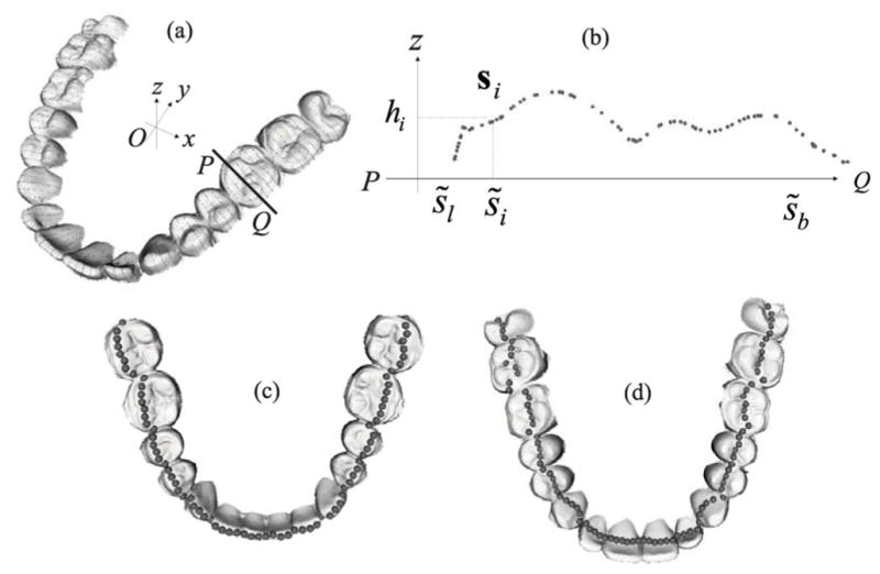
(a) Illustration of intersections (dashed line) of cross-sections and dental surfaces. The occlusal plane is defined by x-O-y plane. (b) The cross-sectional view ( $\overline{PQ}$) of the intersection. {s̃_i} is the projections of {s_i} onto the 1-D coordinate of $\overline{PQ}$, and {h_i} is the corresponding height. s̃_b and s̃_l are the most buccal and lingual values of {s̃_i}. (c) Feature points acquired based on cusps and incisal edges of the mandibular model.(d) Feature points acquired based on central grooves, valleys, and pits of the maxillary model.

1) Feature Points in the Mandibular Model

The feature points on the posterior teeth are the peaks on the buccal cusps, and each of them can be identified by

$$\widehat{i}=arg\underset{i\in S({\stackrel{\sim }{s}}_{\lambda },{\stackrel{\sim }{s}}_b)}{max}{h}_i$$ (1)

where we choose λ = 0.6 to identify buccal peaks at the buccal side of teeth. The feature points on the anterior teeth are the peaks of canines and incisors, and each of them is determined by

$$\widehat{i}=arg\underset{i\in S({\stackrel{\sim }{s}}_l,{\stackrel{\sim }{s}}_b)}{max}{h}_i.$$ (2)

Fig. 5(c) shows the feature points calculated in a mandibular model.

2) Feature Points in the Maxillary Model

The feature points on the posterior teeth are the central grooves and valleys between the buccal and lingual peaks. Let the ĵ = arg max_{i∈S(s̃l, s̃λ)} h_i with λ = 0.4 be the feature point on the lingual cusps. Each of feature points on the central groove can be calculated by

$$\widehat{k}=arg\underset{i\in S({\stackrel{\sim }{s}}_{\widehat{j}},{\stackrel{\sim }{s}}_{\widehat{i}})}{min}{h}_i$$ (3)

where î is calculated in the maxillary model using the same rule as (1). The maxillary anterior teeth, however, do not possess deep grooves and valleys. Instead, the lingual side of incisors and canines is characteristic of visible convex surfaces and pits. Since the bending rate on the lingual surface of anterior teeth is not large enough to detect the pits, we calculate approximate feature points of anterior teeth as follows. Let h̄ be the averaged height of all the feature points of posterior teeth calculated by (3). We choose the feature points which are the closet to the plane z = h̄

$$\widehat{k}=arg\underset{i\in S({\stackrel{\sim }{s}}_l,{\stackrel{\sim }{s}}_{\widehat{i}})}{min}\mid h_i-\overline{h}\mid$$ (4)

where ī is calculated in the maxillary model using the same rule as (2), which corresponds to peaks of anterior teeth. Finally, the feature points of anterior teeth are shifted by l_c in the lingual direction while their heights remain unchanged. l_c is 2 mm for the feature point at the midline and decreased linearly in both the distal directions for the feature points of anterior teeth until l_c is 0 mm for the feature points at Point D and E of Fig. 4(a) (the interstices between the canines and the first premolars). Fig. 5(d) shows the feature points calculated in a maxillary model.

B. Point Matching Algorithm

Let ${\{{\mathbf{p}}_i\}}_{i=0}^{N-1}$ and ${\{{\mathbf{q}}_j\}}_{j=0}^{K-1}$ be sets of 3-D feature points of the maxillary and mandibular dental models. The two sets of points are then matched by applying a point matching approach as if the dental curves fit together when dental models are in the MI. The following point matching algorithm is based on graduated assignment combining “softassign” method [19] and a weighted least squares optimization [20]. The initial alignment becomes to find a transformation and a correspondence between the two sets of feature points {p_i} and {q_j} and minimize an energy function. We calculate a rotation matrix R, a translation vector t, and correspondence [M]_ij ≡ m_ij which minimize

$$\begin{gathered} \sum _{i=0}^{N-1}\sum _{j=0}^{K-1}{m}_{ij}{\Vert {\mathbf{p}}_i-\mathbf{t}-\mathbf{R}{\mathbf{q}}_j\Vert }^2 \\ -\alpha \sum _{i=0}^{N-1}\sum _{j=0}^{K-1}{m}_{ij} \\ \text{subject}\text{to}\sum _{i=0}^{N-1}{m}_{ij}\le 1,\forall j,\sum _{j=0}^{K-1}{m}_{ij}\le 1,\forall i,m_{ij}\in \{0,1\},\forall i,j \end{gathered}$$ (5)

α a threshold biasing the objective function and rejecting outliers. When ||p_i − t − Rq_j||² < α, m_ij = 1 is preferred to m_ij = 0 for minimization of the objective function if all other m’s are zero in the ith row and the jth column. Hence, the pair p_i and q_j will not be treated as outliers with respect to each other. The graduated assignment algorithm determines the correspondence matrix M and solves the transformation {R, t} in an iterative manner. After either correspondence matrix or the transformation is obtained, it can be easily used to determine the other. Given the correspondence matrix, minimization of the energy function in (5) becomes a weighted least square optimization.

The most challenging problem of minimizing (5) is to find a good correspondence matrix. To illustrate the method of point match, we consider only the equalities in the constraints of (5) and a square correspondence matrix. The correspondence matrix becomes a permutation matrix whose entries are either 0 or 1 and has only one 1 in each row and column. Assume constraints on the correspondence matrix with positive integer numbers are relaxed to be positive continuous real numbers. The correspondence matrix becomes a doubly stochastic matrix with all positives continuous entries and rows and columns summing to one. Based on the concept proven by Sinkhorn [21] that a doubly stochastic matrix can be obtained by iteratively performing alternate row and column normalizations of any square matrix with all positive entries, the initial square matrix with all positive entries can be assigned as m_ij = exp[β(α − ||p_i − t − Rq_j||²)] where β > 0 is a control parameter. As β → ∞, the exponentiation makes the maximum entry max_j m_ij in a row be equal to 1 and the other entries become 0 during the process of row normalizations. The same is true to the columns. The doubly stochastic matrix obtained by Sinkhorn’s iterative method will be approximately a permutation matrix if β is large enough. Therefore, a deterministic annealing method can be applied by increasing β for the sake of getting more chances of jumping out the local minima in the point matching optimization. The inequality constraints have to be considered in order to discard the outliers. By introducing positive slack variables m_Nj and m_iK, the inequalities in (5) can be rewritten as

$$\begin{gathered} \sum _{i=0}^N{m}_{ij}\le 1,0\le j\le K-1 \\ \sum _{j=0}^K{m}_{ij}\le 1,0\le i\le N-1. \end{gathered}$$ (6)

The correspondence matrix is unknown at the beginning of the point matching algorithm and has to be estimated appropriately based on the criteria of dental occlusion. Fig. 6(a) shows a proper situation when we perform the point matching algorithm on these feature points. The set of feature points on the arch of the mandibular model is about to match that of the maxillary model in the MI. The situations illustrated in Fig. 6(b) do not happen in real life. However, it may happen during the computation because the dental curves are relatively flat and symmetric with respect to the central incisal midline. The correspondence matrix is calculated only based on the feature points and without considering the other characteristics of the whole models. They should be prevented during the initial alignment. In order to prevent the situation of Fig. 6(b), we take the occlusal planes of the dental models into account.

Fig. 6.

(a) The dental models are properly articulated when the feature points are matched. (b) The articulation is falsely made, even though the feature points of the models are matched. (c) The normal vector of the occlusal plane in the maxillary dental model. (d) The normal vector of the occlusal plane in the mandibular dental model.

Let n_u and n_v be the unit normal vectors of occlusal planes (defined in Section III-A) of the maxillary and mandibular models, shown in Fig. 6(c) and (d). The directions of the normal vectors are from tooth root toward tip. When $-1<{\mathbf{n}}_u^T{\mathbf{n}}_v\le 0$, the occlusal surfaces of the dental models tend to face each other. When $0<{\mathbf{n}}_u^T{\mathbf{n}}_v\le 1$, they exhibit a tendency toward the same direction. Once the rotation matrix R and translation vector t are calculated during the iteration, it is more likely to have the situation of Fig. 6(b) in the following executions of the iteration if ${\mathbf{n}}_u^T{\mathbf{n}}_v^{\prime }>0$, where ${\mathbf{n}}_v^{\prime }=\mathbf{R}{\mathbf{n}}_v$. Therefore, we execute the following step immediately after the transformation {R, t} is calculated each time:

${\mathbf{n}}_v^{\prime }\leftarrow \mathbf{R}{\mathbf{n}}_v$

if ${\mathbf{n}}_u^T{\mathbf{n}}_v^{\prime }>0$ then

− R ← R

end if

Finally, the algorithm is summarized in Algorithm 1. ε₀ is used for convergence criterion and defined as ${\sum }_{i=0}^{N-1}{\sum }_{j=0}^{K-1}{e}_{ij}$ where e_ij is the absolute difference between m_ij at the beginning and upgraded m_ij at the end in the outer while loop ${\epsilon }_0^{\prime }$. is a threshold for convergence. ε₁ and ${\epsilon }_1^{\prime }$ are in the same way and used for the convergence criterion m̃_ij of in the Sinkhorn’s normalization loop (the inner while loop). β_incr is the rate at which control parameter β is increased in the deterministic annealing. A list of these variables and constants are in Table I.

TABLE I.

List of Symbols Appearing in the Point Matching Algorithm

Symbol(s)	Description
β	The control parameter in deterministic annealing
βini	The initial value of the control parameter β
βmax	The ending value of the control parameter β
βincr	The incremental rate of control parameter β
${\epsilon }_0^{\prime }$	The threshold allowed for each value of control parameter β
${\epsilon }_1^{\prime }$	The threshold allowed for row and column normalization
ε0	The variable in the loop for each value of control parameter β
ε1	The variable in the loop of row and column normalization
I0	The maximum number of executions of iteration allowed for each value of control parameter β
I1	The maximum number of executions of iteration allowed for row and column normalization
m̃ij	The variable in the loop of row and column normalization

The sign of rotation matrix R in Algorithm 1 is changed in order to guarantee $-1<{\mathbf{n}}_u^T{\mathbf{n}}_v^{\prime }\le 0$. The purpose of applying deterministic annealing is to seek a good minimum. The execution of this step may increase the chances of being trapped in local minima since the changed transformation does not minimize the objective function given the current correspondence matrix. However, these steps will no longer be executed when β → ∞, i.e., the objective function starts converging. Although robustness of the algorithm is influenced by this modification, the situation of Fig. 6(b) can be prevented.

Algorithm 1.

Point matching algorithm for initial dental alignment

t ← 0, R ← I

for β = βini to βmax do

while ${\epsilon }_0<{\epsilon }_0^{\prime }$ or the number of executions <I0 do

mij ← exp[β(α − ||pi − t − Rqj||2)]

m̃ij ← mij; (Initialization of m̃ij)

while ${\epsilon }_1<{\epsilon }_1^{\prime }$ or the number of executions <I1 do

${\stackrel{\sim }{m}}_{ij}\leftarrow ({\stackrel{\sim }{m}}_{ij})/({\sum }_{i=0}^N{\stackrel{\sim }{m}}_{ij})$, ∀j; (Row normalization)

${\stackrel{\sim }{m}}_{ij}\leftarrow ({\stackrel{\sim }{m}}_{ij})/({\sum }_{j=0}^K{\stackrel{\sim }{m}}_{ij})$, ∀i; (Column normalization)

end while

mij ← m̃ij

Calculate R and t using mij

${\mathbf{n}}_v^{\prime }\leftarrow \mathbf{R}{\mathbf{n}}_v$

if ${\mathbf{n}}_u^T{\mathbf{n}}_v^{\prime }>0$ then

− R ← R

end if

end while

β ← βincrβ

end for

IV. Dental Alignment Using Iterative Surface-Based Minimum Distance Mapping

After the dental models are aligned to an approximate occlusion, they are finally articulated digitally using an algorithm called iterative surface-based minimum distance mapping (ISMDM). The criterion based on maximal contact of the teeth at MI is the key to develop the ISMDM. The articulation of the dental models can be modeled by consecutive executions of translation and rotation and continuous changes of rotational origin on the dental model. In order to automatically achieve maximal contact between upper and lower teeth and reach the final occlusion in the MI, we model this movement by iteratively minimizing distance of surfaces between lower and upper teeth and updating the transformation. This method is based on the idea of the iterative closest point algorithm [22] that is generally used in shape matching, registration, and alignment of two similar datasets from the same object. In addition, an important component in this method is that we add constraints to prevent the two opposite surfaces from overlap. The detailed computational algorithms are described as follows.

A. Modelling of Dental Occlusion

Let ${\{{\mathbf{u}}_i\}}_{i=0}^{M-1}$ and ${\{{\mathbf{v}}_j\}}_{j=0}^{J-1}$ be two sets of M and J vertices of teeth in the digital maxillary and mandibular dental models, respectively. In the following, we assume the maxillary model is in a static position. The transformation is performed on the mandibular model. The transformed v_j is modeled as

$${\mathbf{v}}_j^{\prime }(\stackrel{\sim }{\mathbf{R}},\stackrel{\sim }{\mathbf{t}})\equiv \stackrel{\sim }{\mathbf{R}}({\mathbf{v}}_j-\stackrel{\sim }{\mathbf{o}})+\stackrel{\sim }{\mathbf{o}}+\stackrel{\sim }{\mathbf{t}}$$ (7)

where õ is a rotational origin (the pivot point) of the rotation matrix R̃, and t̃ is the translation vector. Under the assumption that the two digital dental models do not overlap, maximizing contact area is equivalent to maximizing the number of contacting vertices in {v_j}. However, not every vertex in {v_j} will make contact when the models are in the MI. Those contact areas are even more difficult to be predicted precisely. Therefore, we model the distance of surfaces between lower and upper teeth as

$$d_S\equiv \sqrt{\frac{1}{J}\sum _{j=0}^{J-1}{\Vert {\mathbf{u}}_{i_j}-{\mathbf{v}}_j\Vert }^2}$$ (8)

u_ij is a point closest to v_j and is given by

$${\mathbf{u}}_{i_j}=arg\underset{\mathbf{u}\in \{{\mathbf{u}}_i\}}{max}\Vert \mathbf{u}-{\mathbf{v}}_j\Vert$$ (9)

where i_j ∈ {0, 1, …, M − 1}. Instead of directly maximizing contact area, we increase the chances of making contact by minimizing d_S. The rotational origin õ is given by

$$\stackrel{\sim }{\mathbf{o}}=arg\underset{\mathbf{v}\in \{{\mathbf{v}}_j\}}{min}\left(\underset{\mathbf{u}\in \{{\mathbf{u}}_i\}}{min}\Vert \mathbf{u}-\mathbf{v}\Vert \right).$$ (10)

Fig. 7(a) shows surfaces of upper and lower teeth are closer at one side than the other side. Intuitively, rotational origin will be set at the closer side so that the surface of the lower teeth at the contralateral¹⁴ side can be swung closer towards the upper teeth. Because of the irregularity of teeth surfaces, dynamic change of the rotational origin by (10) will enable a better occlusion of lower and upper teeth surfaces.

Fig. 7.

(a) Surfaces of upper and lower teeth are closer at the anterior teeth than the posterior teeth. The rotational origin should be always updated and assigned near the anterior teeth of dental models in order to gain more freedom of articulation. (b) A constraint of (11) is a half-space defined by a plane ℘_j. The transformed vertex ${\mathbf{v}}_j^{\prime }(\stackrel{\sim }{\mathbf{R}},\stackrel{\sim }{\mathbf{t}})$ is not allowed to be in the other half-space, avoiding overlap of upper and lower teeth.

Adding collision constraints is the most important step in digital dental occlusion. We create a mechanism of avoiding collision in 3-D dental datasets. The avoidance of collision is formulated as constraints and will be incorporated into the optimization programming. Fig. 7(b) illustrates how a constraint is imposed. For each pair of points v_j and u_ij, we create a plane between them. Let ℘_j be a plane with a unit normal vector n_j and a point r_j on it. When the transformed vertex ${\mathbf{v}}_j^{\prime }(\stackrel{\sim }{\mathbf{R}},\stackrel{\sim }{\mathbf{t}})$ is not allowed to be at the opposite side of the plane, the constraint can be expressed as

$${[{\mathbf{v}}_j^{\prime }(\stackrel{\sim }{\mathbf{R}},\stackrel{\sim }{\mathbf{t}})-{\mathbf{r}}_j]}^T{\mathbf{n}}_j>0.$$ (11)

r_j can be given by

$${\mathbf{r}}_j={\mathbf{u}}_{i_j}-\delta {\mathbf{n}}_j$$ (12)

where δ is allowable penetration depth. The vertices of lower teeth are allowed to penetrate through the upper teeth surface with depth δ. The calculation of the unit normal vector n_j is demonstrated as follows. Since the datasets are triangulated surfaces, the vertex u_ij is shared with a number of adjacent facets. Let the unit normal vector of the kth facet sharing the vertex u_ij be ${\mathbf{n}}_j^{(k)}$. The n_j is determined by

$${\mathbf{n}}_j=\frac{{\sum }_k{\mathbf{n}}_j^{(k)}}{\Vert {\sum }_k{\mathbf{n}}_j^{(k)}\Vert }$$ (13)

which is Mean Weighted Equally computation of normal. Since most of the areas between upper and lower teeth will never make contact during the MI, a large number of constraints added to the algorithm may be redundant. In order to reduce the number of constraints, it is not necessary to add a constraint to a point pair v_j and u_ij if the distance between them is beyond a threshold ρ

B. Minimization of the Distance of Occlusal Surfaces and the Algorithm

Given a rotational origin õ, we calculate the rotation matrix R̃ and the translation vector t̃ which minimize

$$\begin{gathered} d_S^2(\stackrel{\sim }{\mathbf{R}},\stackrel{\sim }{\mathbf{t}})\equiv \frac{1}{J}\sum _{j=0}^{J-1}{\Vert {\mathbf{u}}_{i_j}-{\mathbf{v}}_j^{\prime }(\stackrel{\sim }{\mathbf{R}},\stackrel{\sim }{\mathbf{t}})\Vert }^2 \\ \text{subject}\text{to}{[{\mathbf{v}}_j^{\prime }(\stackrel{\sim }{\mathbf{R}},\stackrel{\sim }{\mathbf{t}})-{\mathbf{r}}_j]}^T{\mathbf{n}}_j>0. \end{gathered}$$ (14)

The rotation matrix consists of nonlinear terms which can be linearized by small-angle approximation [23], [24]. When the two dental models are getting occluded, the increment needed to seat the dental occlusion will gradually become smaller. Therefore, errors caused by this approximation will become less significant. Approximate the rotational matrix R̃ by linearizing it as

$$\stackrel{\sim }{\mathbf{R}}=\left(\begin{array}{ccc}1& -{\theta }_z& -{\theta }_y\\ {\theta }_z& 1& -{\theta }_x\\ {\theta }_y& {\theta }_x& 1\end{array}\right)$$ (15)

where θ_x, θ_y, and θ_z are rotational angles with respect to x-, y-, and z-axes. Define θ = (θ_x, θ_y, θ_z)^T and L_j as

$${\mathbf{L}}_j=\left(\begin{array}{ccc}0& -v_{j,z}+{\stackrel{\sim }{o}}_z& -v_{j,y}+{\stackrel{\sim }{o}}_y\\ -v_{j,z}+{\stackrel{\sim }{o}}_z& 0& v_{j,x}-{\stackrel{\sim }{o}}_x\\ v_{j,y}-{\stackrel{\sim }{o}}_y& v_{j,x}-{\stackrel{\sim }{o}}_x& 0\end{array}\right).$$ (16)

(R̃ − I)(v_j − õ) can be rewritten as

$$(\stackrel{\sim }{\mathbf{R}}-\mathbf{I})({\mathbf{v}}_j-\stackrel{\sim }{\mathbf{o}})={\mathbf{L}}_j\theta .$$ (17)

The objective function in (14) becomes

$$d_S^2(\stackrel{\sim }{\mathbf{R}},\stackrel{\sim }{\mathbf{t}})=\frac{1}{J}\sum _{h=0}^{J-1}\Vert {\mathbf{L}}_j\theta +\stackrel{\sim }{\mathbf{t}}+{\mathbf{b}}_j{\Vert }^2$$ (18)

where b_j = v_j − u_ij. Let x ≡ (t^T, θ^T) = (t̃_x, t̃_y, t̃_z, θ_x, θ_t, θ_z)^T and ${\stackrel{\sim }{\mathbf{L}}}_j\equiv [\begin{array}{cc}{\mathbf{L}}_j& \mathbf{I}\end{array}]$. Equation (18) becomes (without the scaling 1/J)

$${\mathbf{x}}^T\left(\sum _{j=0}^{J-1}{\stackrel{\sim }{\mathbf{L}}}_j^T{\stackrel{\sim }{\mathbf{L}}}_j\right)\mathbf{x}+2\left(\sum _{j=0}^{J-1}{\mathbf{b}}_j^T{\stackrel{\sim }{\mathbf{L}}}_j\right)\mathbf{x}+\sum _{j=0}^{J-1}{\Vert {\mathbf{b}}_j\Vert }^2.$$ (19)

With the linearization of rotation matrix, the objective function $d_S^2$ becomes a quadratic form, and (11) becomes a linear constraint. The minimization of (14) can be solved by quadratic programming. The algorithm is summarized in Algorithm 2. S the total number of executions in the iteration. ρ is the threshold for limiting the number of linear constraints.

Algorithm 2.

ISMDM algorithm

for k = 0 to S − 1 do

for j = 0 to J − 1 do

uij ← arg maxu∈{ui} ||u − vj||

end for

õ ← arg minv∈{vj}(minu∈{ui} ||u − v||)

for j = 0 to J − 1 do

if ||uij − vj|| < ρ

Add the linear constraint ${[{\mathbf{v}}_j^{\prime }(\stackrel{\sim }{\mathbf{R}},\stackrel{\sim }{\mathbf{t}})-{\mathbf{r}}_j]}^T{\mathbf{n}}_j>0$

end if

end for

Minimize (14) by quadratic programming

Update vj using (7)

end for

V. Validations and Results

Twelve sets of the digital dental models are used in the simulation. They are randomly selected from our clinical archive database using a random number table. The selection criteria include:

1. no early contact;

2. the patients underwent a single-piece maxillary surgery;

3. the models have a stable occlusion.

All the dental models have relatively normal dentition except two pairs of dental models are partial edentulous (Fig. 8) and two pairs of models have first premolar extractions for orthodontic treatment. The occlusion at the MI is established by an experienced CMF surgeon (J. J. Xia). The models are scanned at MI position using a laser scanner as a part of our clinical routine (described in Section II). The surface datasets of the maxillary and mandibular models are saved in .STL format with a resolution of 0.1 mm. In this simulation, they are decimated to a resolution of 0.2 mm. The teeth, which are involved in occlusion, are segmented from the rest of the model. These originally scanned digital models at MI position serve as a control group during the validation processes.

Fig. 8.

Two sets of partial edentulous dental models. (a) and (b) First set of the mandibular and maxillary models, and (c) and (d) are the second set of the mandibular and maxillary models.

The origin O of the Cartesian coordinate system is the centroid of the boundary box of the mandibular model in the control group [Fig. 9(a)], which is determined by the maximum and minimum of the range in the x- (mediolaterally), y- (anteroposteriorly), and z- (superoinferiorly) directions. Three landmarks that are commonly used in clinical practice are selected on the occlusal surface on the mandibular model. They are the mesiobuccal¹⁵ cusp of the first right molar (A), the mesiobuccal cusp of the first left molar (B), and the central dental midline (C). The coordinates of these landmarks are used later to compare with the same landmarks in the experimental group.

Fig. 9.

(a) The Cartesian coordinate system is defined to represent the sagittal, coronal, and axial planes in the control model. The results are validated in Section V-A at mesiobuccal cusps (Point A and B) of the first molar, the mandibular central dental midline (Point C), and the centroid (Point O) in the control model. (b) In Section V-B, the sagittal angular deviation ω̂_x is defined by the angle between the dashed line and the z-axis. The dashed line is calculated by projecting the z′-axis onto the y-O-z plane.

In order to test our approach, it is necessary to first disrupt this relationship because the maxillary and mandibular digital dental models are scanned in MI. To this end, we first duplicate the scanned mandibular teeth model and its landmarks, and then systematically generate rigid transformations to disarticulate the mandibular teeth model while the maxillary teeth model is kept constant. A total of 80 disarticulations are generated in each set of the models by choosing five rotational matrices and 16 translations of rigid transformation. The rotational origin corresponds to the centroid of the mandibular teeth model. Among five rotational matrices, one rotation matrix is identity, and the other four rotation matrices are calculated by choosing a normalized rotational axis and a rotational angle. Two normalized rotational axes are ( $(\sqrt{2})/(2),(\sqrt{2})/(2)$, 0) and ( $-(\sqrt{2})/(2),(\sqrt{2})/(2)$, 0). Two rotational angles of −(1/3)π and (1/3)π are applied with respect to each of the rotational axes. The translation in z-coordinate is chosen as −10 mm to vertically disarticulate the mandibular model (separate the mandibular model apart from the maxillary model). Then, the translations in x- and y-coordinate are incrementally chosen from −20 mm, −7 mm, 7 mm, to 20 mm. These systematically disarticulated models are enough to represent a patient’s malocclusion caused by CMF deformities. These disarticulated models serve as an experimental group. The landmarks A, B and C, and the centroid O and the x-, y-, and z-coordinates in the control model become A′, B′, and C′, and the centroid O′ and the x′-, y′-, and z′-coordinates in the experimental model.

Once the models are systematically disarticulated, the maxillary and mandibular models in the experimental group are initially articulated using our initial alignment algorithm described in Section III. The parameters used in point matching algorithm are summarized in Table II. They are then finally aligned using our ISMDM algorithm described in Section IV. The following parameters are applied in the ISMDM algorithm: S = 60, ρ = 0.2 mm, and δ = 0.1 mm. Fig. 10 shows an example of the plots of average distance of surface d_S versus iteration k for 12 sets of the models in the simulation of the ISMDM algorithm selected from 80 repeated experiments. During the validation process, the maxillary model remains static while the mandibular model seeks its MI position. Finally, validation is completed by calculating the transitional and rotational deviations of the mandibular models between the control and the experimental groups. Based on our clinical experience and published literature [25], there would be no clinical significance if the translational deviation of the mandibular models between the control the experimental groups is less than 0.5 mm and the angular deviation is less than 1° on sagittal, coronal, and axial planes, respectively.

TABLE II.

Parameter in the Simulation of Initial Alignment

${\epsilon }_0^{\prime }$	${\epsilon }_1^{\prime }$	βini	βmax	βincr	I0	I1	α
0.5	0.05	0.009	50	1.2	30	7	2

Fig. 10.

The plots of d_s (mm) versus iteration k in the simulation of ISMDM for 12 sets of the models. The initial positions of the mandibular models for ISMDM algorithm is calculated as follows: the mandibular models are disarticulated from gold standard using rotational axis ( $-(\sqrt{2})/(2),(\sqrt{2})/(2)$,0), rotational angle, and translation (−20 mm, −20 mm, −10 mm) and then aligned by initial alignment algorithm.

A. Validation 1: Translational Deviations on Mesiobuccal Cusps, Central Dental Midline, and Centroid

In the first validation, we compute the translational deviations (deltas) of the articulated experimental models relative to the control model at the landmarks of mesiobuccal cusps of the first molar, the central dental midline, and the centroid in x-, y-, and z-axis. It generates a total of 11 520 sets of deltas, 960 for each pair of the models. The data is first screened and its distribution is normally shaped. In each pair of the models, we then average the 80 repeated deltas resulted from 80 systematic disarticulations for a given landmark at a given direction. Furthermore, Analysis of Variance (ANOVA) for repeated measures is used to detect whether the delta is statistically different from “0,” a hypothetical ideal number of the delta. It is also used to detected whether there is a statistically significant difference among the three directions (x-, y-, and z-), and the four landmarks [(A′, A), (B′, B), (C′, C), and (O′, O)] in final results calculated by the ISMDM algorithm. The result shows the delta is no statistically significantly diverged from “0” [F(1, 11)] = 2.58, P = 0.14] in Fig. 11(a). The results also show there is no statistically significantly difference among three directions [F(2, 22)] = 0.77, P = 0.48], or four landmarks [F(3, 33)] = 0.13, P = 0.94]. Finally, the mean translational deltas, the standard deviations (SDs) and the 95% of confidence intervals (CIs) for the results calculated by the initial alignment algorithm (“Initial alignment”) and for the final results calculated by the ISMDM algorithm (“ISMDM”) are presented in Table III. They indicate that the models are articulated successfully with a small degree of translational deviation.

Fig. 11.

(a) Mean translational deviations (deltas) for each landmark between the experimental and control groups in x-, y-, and z-directions. (b) Mean rotational deviations (deltas) between the experimental and control groups in angular deviations ω̂_x, ω̂_y and ω̂_z.

TABLE III.

Translational Deviations in the Simulation of Initial Alignment and ISMDM

		Initial alignment			ISMDM
		Mean	SD	95% of CI	Mean	SD	95% of CI
(A′, A)	x	−0.068	0.536	(−0.409, 0.272)	−0.086	0.318	(−0.288, 0.116)
	y	0.548	1.224	(−0.230, 1.325)	−0.144	0.636	(−0.548, 0.260)
	z	1.436	0.682	(1.002, 1.870)	−0.065	0.169	(−0.172, 0.042)
(B′, B)	x	−0.128	0.539	(−0.471, 0.214)	−0.098	0.327	(−0.306, 0.110)
	y	0.535	0.979	(−0.087, 1.157)	−0.131	0.440	(−0.410, 0.149)
	z	1.443	0.538	(1.101, 1.786)	0.003	0.100	(−0.060, 0.065)
(C′, C)	x	−0.116	0.747	(−0.951, 0.358)	−0.090	0.378	(−0.331, 0.150)
	y	0.583	0.681	(0.150, 1.015)	−0.130	0.220	(−0.269, 0.010)
	z	0.334	0.697	(−0.108, 0.777)	−0.108	0.332	(−0.320, 0.103)
(O′, O)	x	−0.087	0.387	(−0.333, 0.159)	−0.082	0.225	(−0.226, 0.060)
	y	0.626	0.637	(0.221, 1.031)	−0.132	0.180	(−0.246, −0.018)
	z	1.175	0.429	(0.902, 1.447)	−0.050	0.105	(−0.114, 0.020)

B. Validation 2: Angular Deviations

In the second validation, angular deviations are computed in view of sagittal (y-O-z plane), coronal (x-O-z plane), and axial planes (x-O-y plane) of the control model. The experimental models are moved translationally so that the centroid O′ is matched to the centroid O in the control group. The sagittally angular deviation is then calculated as follows. z′-axis is projected onto the y-O-z plane. We define an angular deviation ω̂_x by calculating the angle between the projected z′-axis and the z-axis. Fig. 9(b) illustrates the projected z′-axis (the dashed line) and a sagittal angular deviation ω̂_x. Similarly, we project the z′-axis onto the x-O-z plane, and the coronal angular deviation ω̂_y is determined by the angle between the projected z′-axis and z-axis. By projecting the y′-axis onto the x-O-y plane, the axial angular deviation ω̂_z is defined by the angle between the projected y′-axis and y-axis. It generates a total of 2880 sets of deltas, 240 for each pair of the models. The data is first screened and its distribution is normally shaped. In each pair of the models, we then average the 80 repeated deltas resulted from 80 systematic disarticulations for a given landmark at a given direction. Furthermore, ANOVA for repeated measures is used to detect whether the delta is statistically different from “0,” a hypothetical ideal number of the delta. It is also used to detected whether there is a statistically significant difference among the three directions (ω̂_x, ω̂_y, and ω̂_z) in final results calculated by the ISMDM algorithm. The results show the delta is not statistically significantly diverged from “0” [F(1, 11) = 0.32, P = 0.58] in Fig. 11(b). The results also show there is no statistically significantly difference among the three directions [F(2, 22) = 0.16, P = 0.84]. Finally, the mean angular deltas, the SDs and the 95% of CIs for the results calculated by the initial alignment algorithm (“Initial alignment”) and for the final results calculated by the ISMDM algorithm (“ISMDM”) are presented in Table IV. They also indicate that the models are articulated successfully with a small degree of rotational deviation.

TABLE IV.

Angular Deviations in the Simulation of Initial Alignment and ISMDM

	Initial alignment			ISMDM
	Mean	SD	95% of CI	Mean	SD	95% of CI
ω̂x	−2.324	2.13	(−3.677, −0.971)	−0.185	0.792	(−0.688, 0.319)
ω̂y	0.006	0.474	(−0.295, 0.307)	−0.100	0.162	(−0.203, 0.004)
ω̂z	0.022	2.112	(−1.319, 1.364)	−0.014	1.234	(−0.799, 0.77)

VI. Discussion

We have developed an automatic and robust approach to digitally articulate dental models. This approach consists of two major steps. The first step is the initial alignment, in which the point match algorithm is used to match the feature points of dental curves in order to bring the models relatively close to each other. The second step is the final alignment, in which we develop the ISMDM algorithm to minimize the average distance of surfaces of the models in order to articulate the maxillary and mandibular models to the MI without overlapping each other. This approach has been validated using 12 pairs of the dental models. The results of validation shows the models are successfully articulated with a small degree of deviation. The accurate results can be attributed to the intuitive assumption that maximizing contact areas of upper and lower teeth is equivalent to minimizing the average distance defined in (8).

The results of the validation show the robustness of our approach. First, the initial alignment algorithm can bring the models to proper positions even before performing the ISMDM. Shown in Tables III and IV, the models aligned by the initial alignment algorithm are close enough to successfully complete final articulation by the ISMDM. Second, each mandibular model is docked to a final occlusion since the average distance of surface d_S converges at k < 30 (illustrated in Fig. 10) using our ISMDM algorithm. Shown in Tables III and IV, the deviations are small enough to satisfy clinical requirements. They demonstrate the feasibility of our approach towards fully automatic digital dental articulation. In addition, our validation includes the models with special conditions: partial edentulous dentition and first premolar extraction due to orthodontic treatment. We initially expect these models may result in a larger deviation. However, even with the models with special conditions, the models in experimental group still achieve a same small degree of deviation. This further proves the robustness of our approach. Of the note a small portion of results of the y-axis (under “ISMDM” in Table III) shows the standard deviations of Point A and B are slightly larger (close to 0.5 mm) than the others. This contributes to a larger range of angular deviation ω̃_z on the axial plane (under “ISMDM” in Table IV). During the dental articulation, the mandibular models have more rotational freedom on the axial plane in comparison to the sagittal and coronal planes. A possible solution to reduce the rotational freedom on the axial plane is to add more constraints, i.e., coincidence between maxillary and mandibular dental midlines.

Our initial alignment algorithm plays an important role in reducing the number of executions of nearest point searching of ISMDM. The high-quality dataset of digital dental models may drastically increase the computational time in ISMDM since the calculation of nearest point searching is tremendous. Our initial alignment algorithm is designed to bring the high-resolution digital dental models used in our clinic to an approximate MI position and orientation, without considering whether there is a collision between the upper and the lower teeth. The advantage of using initial alignment is to tremendously increase the computational speed of convergence in final alignment using ISMDM algorithm and significantly reduce the computational time in planning the CMF surgeries. As illustrated in Fig. 10, all the models can be quickly articulated in only 30 executions of iteration in ISMDM without intensively searching for the position at MI. In our simulation, the computational time of both initial alignment algorithm and the ISMDM for each set of the models is only several minutes.

Our final alignment is to bring the dental models from the position achieved by initial alignment to their final occlusion at the MI and free of collision using our ISMDM algorithm. In this algorithm, the convergence in average distance of surface between the models can be used to decide whether the models have been articulated. The correspondence of vertices in upper and lower teeth and linear constraints are dynamically updated in each iteration, resulting in different parameters of quadratic programming in (19). In this algorithm, the optimal transformation is solved by quadratic programming in each iteration. When the maxillary and mandibular models are getting closer to be articulated, the optimal transformation approximates a null since these linear constraints prevent the models from overlap and stop the models. Once this is achieved, the null transformation will not further update the correspondence and constraints in following iterations. Thus, the average distance will converge.

The final alignment should be completed without overlapping between the upper and the lower models. Another advantage of our ISMDM algorithm is that it has successfully overcome the notorious problem of uncontrollable overlap by applying linear constraints and allowable penetration depth δ. Each of the constraints is determined by one vertex in the upper teeth and its corresponding vertex in the lower teeth. Therefore, the number of constraints depends on the parameter ρ and resolution of datasets. However, the models may not be able to entirely articulate if too many constraints are incorporated in quadratic programming. As we observed, an appropriate value of the parameter ρ is approximate to the resolution of dataset. Theoretically, the penetration depth is zero, leading to no overlap of upper and lower teeth. However, since the surfaces of the digital models are slightly expanded outward [Fig. 2(b)] due to the process of triangulation, the articulated digital models must have little overlap at the contact areas. Therefore, the choice of the allowable penetration depth relies on the extent of overlap in the dataset. In this experiment, we set the penetration depth was 0.1 mm.

Finally, our approach is different from others. The ultimate goal of our approach is to digitally articulate dental models for patient treatment. Hiew et al. [25] used the right and posterior surfaces of the model bases to perform the dental model alignment. They first trimmed the right and posterior surfaces of the upper and lower plaster model bases so they would be perfectly in the same plane with the teeth in the correct occlusion. After the models were separately digitized, the centroids and normal vectors of these surfaces were calculated by using a K-means plane detection algorithm. This initial step was to align the digital models in anteroposterior (y-axis) and transverse (x-axis) directions. The final alignment was then completed by adjusting one of the models in superoinferior (z-axis) direction. Finally, the vertical alignment was optimized by collision detection, and the transformation was applied to the lower model. However, this approach is not designed based on the occlusal criteria. Thus it is impossible to incorporate their method into the actual surgical planning procedure clinically. Zhang et al. [26] designed a two-stage occlusal analysis algorithm. In the first stage, each vertex of the teeth models is checked whether it is considered as a penetration. In the second stage, the distance of each vertex to the opposing model was calculated, and the color ranges of distance were shown on the 3-D teeth models. The color ranges are useful for manual alignment in the computer, but it still needs iterative process of collision detection and manual transformation of the models. Finally, DeLong et al. [27] utilized a “3-point alignment” method. Three pairs of contacting points on both the upper and lower teeth models were initially identified on the plaster models and then digitized onto the digital models. The points on the lower teeth were aligned using a fitting algorithm to the points on the upper teeth model, and the transformation was applied to the lower model. The established occlusion was then visually checked, and the 3-point alignment method was repeated by selecting different pairs of points until the visual outcome was satisfactory and overlap of the models is free. We had independently developed and tested this method before De-Long et al. published their results. Although this method could bring the upper and lower teeth close to MI, it is almost impossible to be certain that what is seen in the computer truly represents the best possible alignment. Since even a small deviation in the occlusion causes a significant clinical problem, this 3-point alignment may be used as an initial alignment but one should not rely on this method of dental alignment to treat real patients. Comparing to the above methods, our method is more practical and can be immediately used in the patient surgical planning process.

VII. Conclusion

We develop a two-step approach to automatically and digitally articulate the maxillary and mandibular teeth. The first step is the initial alignment that aligns the mandibular dental model relatively closer to the maxillary model in an approximate MI. Two set of feature points of dental curves are extracted. One is the feature points for the curve of central groove and pits of the maxillary dental model, and the other is the feature points for the curve of the cusps and incisal edges of the mandibular dental model. By matching these two set of feature points using point matching algorithm, an initial occlusion can be achieved by intentionally ignoring any possible collision between digital dental models. The second step is the final alignment. We align and fine-tune the initially-aligned models to their final occlusion that is collision-free using our ISMDM algorithm. Two controlling mechanisms are designed. The first is the collision constraints to detect and prevent the penetration between the maxillary and the mandibular dental models. The second is the minimization of average distance of surface between the models in order to articulate the models. These two mechanisms are incorporated into an optimization problem and can be solved by quadratic programming. Our approach is validated by using 12 sets of the dental models. Using our approach, the maxillary and mandibular models can be successfully articulated. There is only a small degree of deviation between the digitally articulated occlusion established with our approach and the scanned occlusion established using the current gold standard. This small degree of deviation does not have clinical significance.

References

- 1.Gateno J, Xia JJ, Teichgraeber JF, Christensen AM, Lemoine JJ, Liebschner MA, Gliddon MJ, Briggs ME. Clinical feasibility of computer-aided surgical simulation (CASS) in the treatment of complex cranio-maxillofacial deformities. J Oral Maxillofac Surg. 2007 Apr;65:728–734. doi: 10.1016/j.joms.2006.04.001. [DOI] [PubMed] [Google Scholar]
- 2.Swennen GR, Barth EL, Eulzer C, Schutyser F. The use of a new 3-D splint and double CT scan procedure to obtain an accurate anatomic virtual augmented model of the skull. Int J Oral Maxillofac Surg. 2007 Feb;36(2):146–152. doi: 10.1016/j.ijom.2006.09.019. [DOI] [PubMed] [Google Scholar]
- 3.Xia JJ, Gateno J, Teichgraeber JF. Three-dimensional computer-aided surgical simulation for maxillofacial surgery. Atlas Oral Maxillofac Surg Clin North Am. 2005 Mar;13(1):25–39. doi: 10.1016/j.cxom.2004.10.004. [DOI] [PubMed] [Google Scholar]
- 4.Bell WH, Guerrero CA. Distraction Osteogenesis of the Facial Skeleton. Philadelphia, PA: Decker; 2006. [Google Scholar]
- 5.Xia JJ, Gateno J, Teichgraeber JF. New clinical protocol to evaluate craniomaxillofacial deformity and plan surgical. J Oral Maxillofac Surg. 2009 Oct;64(10):2093–2106. doi: 10.1016/j.joms.2009.04.057. [DOI] [PMC free article] [PubMed] [Google Scholar]
- 6.Gateno J, Xia JJ, Teichgraeber JF, Rosen A. A new technique for the creation of a computerized composite skull model. J Oral Maxillofac Surg. 2003 Feb;61(2):222–227. doi: 10.1053/joms.2003.50033. [DOI] [PubMed] [Google Scholar]
- 7.Swennen GRJ, Mollemans W, Clercq CD, Abeloos J, Lamoral P, Lippens F, Neyt N, Casselman J, Schutyser F. A conebeam computed tomography triple scan procedure to obtain a threeDimensional augmented virtual skull model appropriate for orthognathic surgery planning. J Craniofac Surg. 2009 Mar;20(2):297–307. doi: 10.1097/SCS.0b013e3181996803. [DOI] [PubMed] [Google Scholar]
- 8.Swennen GRJ, Mommaerts MY, Abeloos J, Clercq CD, Lamoral P, Neyt N, Casselman J, Schutyser F. A cone-beam CT based technique to augment the 3-D virtual skull model with a detailed dental surface. Int J Oral Maxillofac Surg. 2009 Jan;38(1):48–57. doi: 10.1016/j.ijom.2008.11.006. [DOI] [PubMed] [Google Scholar]
- 9.Altobelli DE, Kikinis R, Mulliken JB, Cline H, Lorensen W, Jolesz F. Computer-assisted three-dimensional planning in craniosurgical planning. Plast Reconstr Surg. 1993 Sep;92(4):576–585. [PubMed] [Google Scholar]
- 10.Bill J, Reuther JF, Betz T, Dittmann W, Wittenberg G. Rapid prototyping in head and neck surgery planning. J Craniomaxillofac Surg. 1996;24:20–29. [Google Scholar]
- 11.Xia JJ, Ip HHS, Samman N, Wang D, Kot CSB, Yeung RWK, Tideman H. Computerassisted three-dimensional surgical planning and simulation: 3-D virtual osteotomy. Int J Oral Maxillofac Surg. 2000 Feb;29(1):11–17. [PubMed] [Google Scholar]
- 12.Xia JJ, Ip HHS, Samman N, Wong HTF, Gateno J, Wang D, Yeung RWK, Kot CSB, Tideman H. Three-dimensional virtual-reality surgical planning and soft-tissue prediction for orthognathic surgery. IEEE Trans Inf Technol Biomed. 2001 Jun;5(2):97–107. doi: 10.1109/4233.924800. [DOI] [PubMed] [Google Scholar]
- 13.Zachow S, Hege HC, Deuflhard P. Computer-assisted planning in cranio-maxillofacial surgery. J Comput Inf Technol. 2006;14(1):53–64. [Google Scholar]
- 14.Bell WH. Surgical Correction of Dentofacial Deformities. Philadelphia, PA: Saunders; Jun, 1980. [Google Scholar]
- 15.Ash MM, Ramfjord SP. Occlusion. Philadelphia, PA: Saunders; 1995. [Google Scholar]
- 16.Okeson JP. Management of Temporomandibular Disorders and Occlusion. St. Louis, MO: Mosby; 2002. [Google Scholar]
- 17.Kondo T, Ong SH, Foong CKW. Tooth segmentation of dental study models using range images. IEEE Trans Med Imag. 2004 Mar;23(3):350–362. doi: 10.1109/TMI.2004.824235. [DOI] [PubMed] [Google Scholar]
- 18.Zhao M, Ma L, Tan W, Nie D. Interactive tooth segmentation of dental models. Proc. 27th Annu. Int. Conf. Eng. Med. Biol. Soc; 2005; pp. 654–657. [DOI] [PubMed] [Google Scholar]
- 19.Fang JJ, Kuo TH. Computer-aided design tracked motion-based dental occlusion surface estimation for crown restoration. Computer-Aided Design. 2009;41(4):315–323. [Google Scholar]
- 20.Walker MW, Shao L, Volz RA. Estimating 3-D location parameters using dual number quaternions. CVGIP: Image Underst. 1991 Nov;54(3):358–367. [Google Scholar]
- 21.Sinkhorn R. A relationship between arbitrary positive matrices and doubly stochastic matrices. Ann Math Statist. 1964;35(2):876–879. [Google Scholar]
- 22.Besl PJ, McKay HD. A method for registration of 3-D shapes. IEEE Trans Pattern Anal Mach Intell. 1992 Feb;14(2):239–256. [Google Scholar]
- 23.Milenkovic VJ, Schmidl H. Optimization-based animation. Proc. 28th Annu. Conf. Comput. Graph. Interactive Tech; 2001; pp. 37–46. [Google Scholar]
- 24.Zhang L, Kim YJ, Varadhan G, Manocha D. Generalized penetration depth computation. Computer-Aided Design. 2007 Aug;39(8):625–638. [Google Scholar]
- 25.Hiew LT, Ong SH, Foong KWC. Optimal occlusion of teeth. Proc. 9th IEEE Int. Conf. Control, Automat., Robot., Vis; 2006; pp. 1–5. [Google Scholar]
- 26.Zhang C, Chen L, Zhang F, Zhang H, Feng H, Dai G. A new virtual dynamic dentomaxillofacial system for analyzing mandibular movement, occlusal contact, and TMJ condition. Proc. 1st Int. Conf. Digital Human Model. (ICDHM’07); 2007; pp. 747–756. [Google Scholar]
- 27.Delong R, Ko CC, Anderson GC, Hodges JS, Douglas WH. Comparing maximum intercuspal contacts of virtual dental patients and mounted dental casts. J Prosthetic Dentistry. 2002 Dec;88(6):622–630. doi: 10.1067/mpr.2002.129379. [DOI] [PubMed] [Google Scholar]