Online Cross-Validation-Based Ensemble Learning

Abstract

Online estimators update a current estimate with a new incoming batch of data without having to revisit past data thereby providing streaming estimates that are scalable to big data. We develop flexible, ensemble-based online estimators of an infinite-dimensional target parameter, such as a regression function, in the setting where data are generated sequentially by a common conditional data distribution given summary measures of the past. This setting encompasses a wide range of time-series models and as special case, models for independent and identically distributed data. Our estimator considers a large library of candidate online estimators and uses online cross-validation to identify the algorithm with the best performance. We show that by basing estimates on the cross-validation-selected algorithm, we are asymptotically guaranteed to perform as well as the true, unknown best-performing algorithm. We provide extensions of this approach including online estimation of the optimal ensemble of candidate online estimators. We illustrate excellent performance of our methods using simulations and a real data example where we make streaming predictions of infectious disease incidence using data from a large database.

1 Introduction

Currently the size of data sets is growing faster than the speed of processors. It is now common to encounter data on the order of millions or even billions of observations. In these situations, statistical learning is limited more by computation time than sample size, which has led to increased interest in online estimation. Online estimators update a current estimator with a new incoming batch of data without revisiting past data, thereby avoiding the computational limitations associated with big data. As a motivating example, we analyze a database that has recorded the incidence of Hepatitis A over time in several geographic regions. We are interested in developing an algorithm that accurately predicts future incidence of disease based on past incidence. In such prediction problems, the scale of the data may be such that re-computing the prediction algorithm with each batch of incoming data would be prohibitively slow. Online algorithms offer a way to ensure fast updating of predictions as new data is accrued.

There is a growing body of literature describing online algorithms, but little in the literature guides how to select from amongst these algorithms in practice. In the setting of small-scale, independent and identically distributed (i.i.d.) data, cross-validation is used to objectively compare the performance of a library of candidate estimators. Theoretical results guarantee that the estimator that exhibits the best estimated cross-validated performance is asymptotically equivalent with the unknown best estimator in the library (van der Laan and Dudoit, 2003; van der Vaart et al., 2006; van der Laan et al., 2006). These results extend to the best ensemble (i.e., weighted combination) of candidate estimators. Due to this theoretical property, these estimators have been referred to as super learners (van der Laan et al., 2007). In practice, super learning has been shown to be effective in many settings, including prediction of mortality among the elderly (Rose, 2013) and mortality in the ICU (Pirracchio et al., 2015). However, in the setting of big or streaming data, the existing super learning approach is limited by the computational expense of performing cross-validated estimator selection de novo with each incoming batch of data. Furthermore, the approach is not applicable in dependent data settings. Thus, we require new developments to perform scalable cross-validated estimator selection and ensemble learning.

In this work, we propose an online form of cross-validation that is used to identify the best candidate online algorithm in a library of candidate algorithms. We establish oracle inequalities that show that the performance of the estimator based on the cross-validation-selected best algorithm is asymptotically equivalent with the performance of the unknown best candidate estimator. This allows researchers to posit many different algorithms for estimation, learn in real time which algorithm is best, and base future estimates on this algorithm. We also propose an online method for identifying the best ensemble of the candidate online estimators. We provide a further extension relevant for i.i.d. observations and relate the results to existing oracle inequalities established for standard forms of offline cross validation.

The outline of the remainder is as follows. We formulate the general statistical estimation problem in Section 2 and review key concepts from the online literature in Section 3. In Section 4, we introduce online cross-validation and discuss how it is used to identify the best-performing online estimator from many candidate estimators. We discuss the optimality of the cross-validation-selected estimator by comparing its performance to that of the unknown best-performing algorithm. In this section, we also extend our estimator to allow for online estimation of the optimal ensemble of all candidate online algorithms. In Section 5, we conduct a simulation study and in Section 6, we apply our methods to a data set where the goal is streaming prediction of infectious disease incidence. We conclude with a short discussion.

2 Formulation of the estimation problem

2.1 Statistical model

Suppose at each time t_i, we observe a random variable O(i), i = 1,…, n. In our data analysis, we consider an infectious disease database that records the incidence of Hepatitis A in several geographic regions. Let $P_0^n$ be the true probability distribution of O(1),…, O(n), and let $p_0^n$ be its density with respect to a dominating measure μⁿ. The likelihood of an observation o = {o(1),…, o(n)} is factorized according to time-ordering as follows:

$$p_0^n(o)={\displaystyle \prod _{i=1}^n{p}_{0,i}(o(i)|\overline{O}(i-1)=\overline{o}(i-1))},$$

where we defined Ō(i − 1) = {O(1),…, O(i − 1)}. If we make no further assumptions about $P_0^n$, the statistical estimation problem is intractable – we only have a single observation from $P_0^n$, which limits our ability to learn about the underlying data generating process. The problem could be greatly simplified by making the usual i.i.d. assumption, which would allow us to write

$$p_0^n(o)={\displaystyle \prod _{i=1}^n{p}_{0,i}(o(i)|\overline{O}(i-1)=\overline{o}(i-1))}={\displaystyle \prod _{i=1}^n{\overline{p}}_0(o(i))},$$ (1)

where ${\overline{p}}_0$ is an unconditional density common to each observation. However, in many settings such an independence assumption is not justified. For example, in the infectious disease setting the incidence at a given time Y(i) might depend on past disease incidence. For some diseases, it may be reasonable to assume that the incidence Y(i) is independent of past data conditional on the previous k measurements, Z(i) = {O(j) : j = i − 1, i − 2,…, i − k}. In general, we expect to encounter settings where an observation O(i) is independent of past observations given some fixed-dimension summary of the past data, Z(i) = f_i(Ō(i − 1)),

$$\begin{gathered} p_0^n(o)={\displaystyle \prod _{i=1}^n{p}_{0,i}(o(i)|\overline{O}(i-1)=\overline{o}(i-1))} \\ ={\displaystyle \prod _{i=1}^n}{p}_{0,i}(o(i)|Z(i)=z(i)). \end{gathered}$$

However, with this assumption each observation O(i) still may have a unique conditional distribution. Therefore, we make a stationarity assumption – that is, we assume each observation has a common conditional distribution ${\overline{P}}_0$ given Z. We use ${\overline{p}}_0$ to denote the conditional density of ${\overline{P}}_0$ with respect to a dominating measure μ. We can now express the likelihood of the observed data as

$$\begin{gathered} p_0^n(o)={\displaystyle \prod _{i=1}^n{p}_{0,i}(o(i)|\overline{O}(i-1)=\overline{o}(i-1))} \\ ={\displaystyle \prod _{i=1}^n{p}_{0,i}(o(i)|Z(i)=z(i))} \\ ={\displaystyle \prod _{i=1}^n{\overline{p}}_0(o(i)|Z(i)=z(i))} \end{gathered}$$

This expression makes clear that the conditional density ${\overline{p}}_0$ of each observation does not change over time, though the conditioning set Z will change. Nevertheless, with each observation we gain more information about the common conditional distribution of the data. We define our statistical model ℳ as a collection of possible stationary distributions $\overline{P}$ that could have given rise to the observed data.

Throughout the paper, we used the incidence of infectious disease as a running example for illustrative purposes; however, our framework is quite general and encompasses a wide range of data applications. For example, the assumption of i.i.d. observations, as in equation (1), is a special case where Z(i) = Ø for all i. Therefore, our methodology is applicable to large databases of independent observations. We place no restriction on the dimension of the observation made at each time i. Therefore our framework encompasses the case that a fixed population of N individuals are measured at each time i = 1,…, n. In some cases, we are able to assume that individuals are independent, in which case we observe N independent measurements of the same time series. Our methods are easily modified to handle this case. A more challenging case is when the N individuals are dependent, and thus we only have a single observation of the time series. In this case, our conditional independence assumption states that O(i) = {O_j(i) : j = 1,…, N} is independent of Ō (i − 1) given a fixed-dimensional summary measure of past measurements, Z(i). Another important special case is data generated by a group sequential adaptive design (Chambaz and van der Laan, 2011a,b). In such trials, O(i) = {W(i), A(i), Y(i)}, where W(i) are covariate measurements on the i-th trial enrollee, A(i) is their treatment assignment, and Y(i) is their outcome. The probability that the i-th participant receives treatment is based on Z(i), a summary measure of data collected on past patients. Thus, the distribution of O(i) depends on data collected on past patients, but only through Z(i). Finally, the summary measure Z(i) might include functions of i itself, which allows adjustments for trends over time or seasons.

2.2 Statistical target parameter and loss functions

We are interested in learning about a feature of the true data distribution. To formalize this notion, we call the feature of interest the statistical target parameter and write it as a function Ψ : ℳ → Ψ that takes a distribution $\overline{P}$ from the model and maps it into the parameter space Ψ. In some cases, we may wish to learn about the entire conditional distribution ${\overline{P}}_0$; however, often we are satisfied learning about a summary measure of this distribution. For example, in the infectious disease setting we are occasionally interested in the joint conditional distribution of disease and regional characteristics; however, in many cases we are interested in a summary of this distribution, such as the conditional mean of disease incidence given current regional characteristics and past measurements.

Our method for estimation should reflect the choice of the statistical target parameter. For example, to learn about the conditional mean of disease incidence, we could estimate the joint conditional distribution of regional characteristics and disease incidence, which would imply an estimate of the conditional mean. However, such a procedure is not targeted towards the goal of estimating the conditional mean. To ensure parsimony between our estimation procedure and our target parameter, we introduce the notion of a loss function. Suppose we are interested in estimating the target parameter ${\psi }_0=\mathrm{\Psi }({\overline{P}}_0)$. We call |(Ζ, Ο, ψ) → L(ψ)(Ζ,O) a loss function for ψ₀ if for all z, E₀{L(ψ₀)(Z,O) | Z = z} = min_ψ∈ΨE₀{L(ψ₀)(Z, O) | Z = z}, where we use E₀(·|Z = z) to denote the expectation under ${\overline{P}}_0$ given Z = z. In words, a loss function for a given parameter is defined as a function whose true conditional mean given a summary of the past is minimized by the true value of the parameter.

Returning to the infectious disease example, if we are interested in the full joint conditional density ${\overline{p}}_0$, we could use negative log-likelihood loss, $L(\overline{p})(z,o)=-\mathrm{\text{log}}\{\overline{p}(o|Z=z)\}$. For each z, $E_0[-\mathrm{\text{log}}\{\overline{p}(O|Z)\}|Z=z]$ is minimized by the true conditional density ${\overline{p}}_0$. If instead we are interested in the conditional mean of disease incidence given current regional characteristics and past disease incidence, we could use the squared-error loss, L(ψ)(O, Z) = {Y − ψ(Ζ, W)}². Notice that E₀ [{Y − ψ(Z, W)}² | Z = z] = E₀(E₀[{Y − ψ(Z,W)}² | Z = z, W] | Z = z), where the inner expectation is taken over the conditional distribution of Y given Z = z and W. For every (z, w), the inner expectation is minimized over all ψ ∈ Ψ by ψ₀(z, w) the true conditional mean of Y given Z = z and W = w.

Loss functions play an important role in the development of our methodology in two ways. First, the expectation of a loss function is used to define a theoretical criteria for comparing an estimator and the truth, as we show in the next section. Second, the empirical mean of the loss serves as a criteria for comparing various estimators of the statistical target parameter and we use this fact to develop our estimator.

3 Online estimation

To introduce key concepts in online estimation, we consider the parametric model and i.i.d. regression setting, where Z = Ø and we assume that the mean of Y conditional on W is described by the linear model ψ_β (W) = β′W. This setting has been extensively studied in the online literature in recent years (Zinkevich, 2003; Crammer et al., 2006; Bottou, 2010; Shalev-Shwartz, 2011). Suppose we are interested in ψ₀ (W), the conditional mean of Y given W. In the assumed parametric model, estimating ψ₀ corresponds to estimating β₀ = argmin_βΕ₀{L(ψ_β)(Y, W)} for β₀ ∈ ℝ^d and an appropriate loss function. Define ${\widehat{\beta }}_n$ as minimizer of the empirical average of the loss function,

$${\widehat{\beta }}_n={\mathrm{\text{argmin}}}_{\beta }\frac{1}{n}{\displaystyle \sum _{i=1}^{n}L({\psi }_{\beta })(O(i))}.$$

For example, if we assume the parametric model {p_β : β ∈ ℝ^d} and let L(ψ_β) = − log p_β, then ${\widehat{\beta }}_n$ is the maximum likelihood estimator of β₀.

To study the performance of ${\psi }_{\widehat{\beta },n}$ as an estimator of ψ₀, we construct loss-based dissimilarity measures. The measure $d_{0n}({\psi }_{\widehat{\beta },n},{\psi }_0)=E_0\{L({\psi }_{\widehat{\beta },n})(O)-L({\psi }_0)(O)\}$ compares the true average loss when using ${\psi }_{\widehat{\beta },n}$ to the true average loss when using ψ₀. This measure is decomposed further:

$$d_{0n}({\psi }_{\widehat{\beta },n},{\psi }_0)=E_0\{L({\psi }_{\beta ,0})(O)-L({\psi }_0)(O)\}=E_0\{L({\psi }_{\widehat{\beta },n})(O)+L({\psi }_{\beta ,0})(O)\}=d_{0n}({\psi }_{\beta ,0},{\psi }_0)+d_{0n}({\psi }_{\widehat{\beta },n},{\psi }_{\beta ,0}).$$

The first term is sometimes referred to as the approximation error and describes the average loss incurred by estimating ψ₀ with ψ_β,₀. The second term is referred to as the estimation error and describes the average loss incurred by minimizing empirical rather than true mean of the loss function (Bousquet and Bottou, 2008). In big data settings, computing the true minimizer ${\widehat{\beta }}_n$ is often computationally expensive. Rather than carrying out this minimization with great accuracy, online algorithms may be formulated to approximate the minimum.

Stochastic gradient descent is one such online algorithm, which involves an iterative optimization routine that takes a small step in the direction of the negative gradient of the loss function at a randomly selected observation from the data set. We define the recursive updating step

$${\beta }_{t+1}={\beta }_t-{\gamma }_t{\mathrm{\Gamma }}_t\frac{d}{d{\beta }_t}L({\psi }_{\beta ,t})(O(t))$$ (2)

where γ_t is a scalar step size or learning rate, Γ_t is a d × d matrix, and O(t) is the observation used at the t-th step (Bottou, 2010). In first-order SGD Γ_t is some constant times the identity matrix, while other variants replace Γ_t with an appropriate diagonal matrix (e.g., diagonal elements of the estimated inverse Hessian) (Duchi et al., 2011; Zeiler, 2012). Second-order SGD accounts for the curvature of the loss function by using a Γ_t that approximates the inverse Hessian(Murata, 1999). However, computing and storing an estimate of this matrix is often computationally expensive for high-dimensional d and, though it is optimal, second-order SGD is rarely used in practice. There are many other methods for online optimization that have been used in a variety of contexts (Polyak and Juditsky, 1992; Xu, 2011), including settings with regularized loss functions, such as the Lasso regression and support vector machines (Fu, 1998; Langford et al., 2009; Kivinen et al., 2004; Balakrishnan and Madigan, 2008; Shalev-Shwartz et al., 2011).

Regardless of which method is chosen, after t steps we hope that the approximated minimum is sufficiently close to the true minimum. We can again use loss-based dissimilarities to study the performance of ψ_β,t as an estimator of ψ₀ using

$$d_{0n}({\psi }_{\beta ,t},{\psi }_0)=d_{0n}({\psi }_{\beta ,0},{\psi }_0)+d_{0n}({\psi }_{\widehat{\beta },n},{\psi }_{\beta ,0})+d_{0n}({\psi }_{\beta ,t},{\psi }_{\widehat{\beta },n}),$$

where the first two terms are again the approximation and estimation error, while the new term is the optimization error incurred by using β_t rather than the true minimizer ${\widehat{\beta }}_n$. Existing results in the online learning literature suggest that in big data settings, the estimation and optimization error will be small (Shalev-Shwartz, 2011). Thus, the performance of an online estimator will be determined largely by the approximation error. To minimize the approximation error, we utilize the super learning framework, where we posit a library of candidate estimators for the purpose of estimating ψ₀. It is not possible a-priori to know which estimator will perform best according to our loss-based dissimilarity. However, we can estimate performance of the estimators from the data using cross validation. Cross validation is a sample-splitting technique that involves training a method (e.g., estimating parameters of a parametric model) on a portion of the data, called the training sample, and subsequently evaluating the average loss of those estimators on the withheld portion of the data, called the validation sample. In the following section, we propose an online form of cross validation that we use to evaluate candidate online estimators in the present setting with large-scale, dependent data.

4 Online super learner

4.1 Online cross-validation for dependent data

Suppose we have K candidate estimators ${\widehat{\mathrm{\Psi }}}_k$, k = 1,…, K that can be applied to data sets {Z(i), O(i)} for i ranging over a subset of {1,…, n}. Suppose that these estimators use the first n_ℓ observations to construct initial estimators of ${\widehat{\mathrm{\Psi }}}_k$ and proceed with online updates thereafter. For example, if ${\widehat{\mathrm{\Psi }}}_k$ is based on a parametric model, maximum likelihood estimation could be used based on the first n_ℓ observations to obtain initial estimates of the model’s parameters and stochastic gradient descent used thereafter to provide online updates of the parameter estimates. Typically, n_ℓ is chosen to be as large as is computationally tractable as to minimize optimization error.

To evaluate the performance of different candidate estimators, we use online cross validation to estimate the average loss of each candidate. At time t₀ ∈ {n_ℓ + 1,…, n} we define the data received before t₀ as the training sample, and the singleton O(t₀) as the validation sample. We use this sample splitting to evaluate how well an estimator trained on the past is able to predict an outcome at the next time point.

For each t₀, let $P_{t_0-1}$ denote the empirical distribution of the training sample {Z(i), O(i) : i = 1,…, t₀ − 1} and let ${\widehat{\mathrm{\Psi }}}_{k,t_0-1}={\widehat{\mathrm{\Psi }}}_k(P_{t_0-1})$ denote the estimator ${\widehat{\mathrm{\Psi }}}_k$ trained using {Z(i), O(i) : i = 1,…, t₀ − 1}. Given a candidate estimator ${\widehat{\mathrm{\Psi }}}_k$ we define its online cross-validated risk as

$$R_{\mathit{CV},n}({\widehat{\mathrm{\Psi }}}_k)=\frac{1}{n-n_{\text{ℓ}}+1}{\displaystyle \sum _{t_0=n_{\text{ℓ}}+1}^{n}L({\widehat{\mathrm{\Psi }}}_{k,t_0-1})(Z(t_0),O(t_0))}.$$

Note that if ${\widehat{\mathrm{\Psi }}}_k$ is an online estimator, then the online cross-validated risk is also an online estimator, computed recursively as

$$R_{\mathit{CV},n+1}({\widehat{\mathrm{\Psi }}}_k)=\frac{n-n_{\text{ℓ}}+1}{n-n_{\text{ℓ}}+2}{R}_{\mathit{CV},n}({\widehat{\mathrm{\Psi }}}_k)+\frac{1}{n-n_{\text{ℓ}}+2}L({\widehat{\mathrm{\Psi }}}_{k,n})(Z(n+1),O(n+1)).$$

The proposed cross validation thus proceeds as follows: with each new observation O(t₀+1) create {Z(t₀+1), O(t₀+1)}; evaluate the loss $L({\widehat{\mathrm{\Psi }}}_k(P_{t_0})(Z(t_0+1),O(t_0+1))$ for each k; add this loss to the current estimate of online cross-validated risk; update each online estimator ${\widehat{\mathrm{\Psi }}}_{k,t_0}$ into ${\widehat{\mathrm{\Psi }}}_{k,t_0+1}$ using O(t₀ + 1). Upon receipt of the next observation O(t₀ + 2), the process is repeated.

4.2 Online cross-validation selector and online oracle selector

The online cross-validated risk $R_{\mathit{CV},n}({\widehat{\mathrm{\Psi }}}_k)$ gives an empirical measure of performance for each estimator k = 1,…, K. Based on this measure, we define $k_n={\mathrm{\text{argmin}}}_k{R}_{\mathrm{CV},n}({\widehat{\mathrm{\Psi }}}_k)$ as the online estimator with the best estimated performance, which we refer to as the online cross-validation selector. We can now define a new estimator that at each step t uses the estimates from the online cross-validation selector, $\widehat{\mathrm{\Psi }}(P_t)={\widehat{\mathrm{\Psi }}}_{k_t}(P_t)$, t = 1,…, n. We call this estimator the discrete online super learner. Notice that over time the discrete online super learner could switch from one estimator to another. If all the candidate estimators are online estimators, then the discrete super learner is itself an online estimator and therefore is as scalable as any of the candidate estimators.

We turn to what can be said theoretically about this approach. Our approach to studying the theory of these estimators is based on establishing oracle inequalities. First, we establish a metric that measures how far a given estimator is from the truth. We then define an oracle selector, which is a hypothetical estimator that uses the candidate estimator that is closest to the truth. Though this estimator can not be computed in practice, it serves as a benchmark by which we can compare the performance of our online cross-validation-based estimator. Specifically, we compare the distance between our estimator and the truth to the distance between the oracle estimator and the truth using an inequality. We show that as sample size grows, the ratio of the distances converges to online, which proves that asymptotically the online cross-validation selector is asymptotically equivalent with the oracle estimator.

To establish a relevant metric for comparing estimators, we first note that the online cross-validated risk estimates the following true online cross- validated risk:

$${\stackrel{\sim }{R}}_{\mathit{CV},n}({\widehat{\mathrm{\Psi }}}_k)=\frac{1}{n-n_{\text{ℓ}}+1}{\displaystyle \sum _{t_0=n_{\text{ℓ}}+1}^n{E}_0\{L({\widehat{\mathrm{\Psi }}}_{k,t_0-1})(O(t_0))|Z(t_0)=z(t_0)\}}.$$ (3)

This is the sum over all times of the true average loss for the estimator ${\widehat{\mathrm{\Psi }}}_k$ with respect to the conditional distribution of O(t₀) given Z(t₀) equals the observed value z(t₀) and is minimized by ψ₀. To study how the performance of a particular estimator compares to the true parameter, we define an online loss-based dissimilarity,

$$d_{0n}({\widehat{\mathrm{\Psi }}}_k,{\psi }_0)=\frac{1}{n-n_{\text{ℓ}}+1}{\displaystyle \sum _{t_0=n_{\text{ℓ}}+1}^n{E}_0\{L({\widehat{\mathrm{\Psi }}}_{k,t_0-1})(O(t_0))-L({\psi }_0)(O(t_0))|Z(t_0)=z(t_0)\}}.$$

For certain loss functions, this measure can intuitively be written as a difference between the estimator and the truth. Consider the squared L² distance between ψ and ψ₀ under the conditional distribution ${\overline{P}}_0$ of W(t₀), Y(t₀) given Z(t₀) = z,

$$d_{L2,z}^2(\psi ,{\psi }_0)=E_0[{\{\psi (W,Z)-{\psi }_0(W,Z)\}}^2|Z(t_0)=z)].$$

When considering squared-error loss, the loss-based dissimilarity $d_{0n}({\widehat{\mathrm{\Psi }}}_k,{\psi }_0)$ is

$$d_{0n}({\widehat{\mathrm{\Psi }}}_k,{\psi }_0)=\frac{1}{n-n_{\text{ℓ}}+1}{\displaystyle \sum _{t_0=n_{\text{ℓ}}+1}^n{E}_{W,0}\left[{\{{\widehat{\mathrm{\Psi }}}_{k,t_0-1}(W,Z(t_0))-{\psi }_0(W,Z(t_0))\}}^2\right|Z(t_0)=z(t_0)]}=\frac{1}{n-n_{\text{ℓ}}+1}{\displaystyle \sum _{t_0=n_{\text{ℓ}}+1}^n{d}_{L2,z(t_0)}^2({\widehat{\mathrm{\Psi }}}_{k,t_0-1},{\psi }_0)}.$$

This shows that the loss-based dissimilarity is equal to the sum over the observations of the squared L² distance between ${\widehat{\mathrm{\Psi }}}_k$ and ψ₀, where at each time t₀ the average is computed with respect to the distribution of {W(t₀), Y(t₀)} conditional on Z(t₀) = z(t₀). Similarly, with binary Y and a log-likelihood loss criteria, we can show that $d_{0n}({\widehat{\mathrm{\Psi }}}_k,{\psi }_0)$ has an interpretation as the Kullback-Leibler divergence of ${\widehat{\mathrm{\Psi }}}_k$ and ψ₀ under the conditional distribution of O given Z = z.

We have now argued that the online loss-based dissimilarity is an interesting metric by which we can compare an estimator to true value of the unknown target parameter in the online setting. We therefore consider which of the candidate estimators minimizes this online loss-based dissimilarity and define

$${\stackrel{\sim }{k}}_n=\mathrm{\text{arg}}\underset{k}{\min }\frac{1}{n-n_{\text{ℓ}}+1}{\displaystyle \sum _{t_0=n_{\text{ℓ}}+1}^n{d}_{0n}({\widehat{\mathrm{\Psi }}}_k,{\psi }_0)}.$$

We call this index the online oracle selector. Of course, the oracle selector is unknown in practice as it depends on the true conditional distribution of the data. Nevertheless, we can compare the performance of the online discrete super learner to that of the oracle selector. In Section A of the Appendix, we provide a formal theorem that establishes a finite-sample inequality comparing the discrete online super learner to the online oracle selector. This inequality is used to show that

$$\frac{d_{0n}({\widehat{\mathrm{\Psi }}}_{k_n},{\psi }_0)}{d_{0n}({\widehat{\mathrm{\Psi }}}_{{\stackrel{\sim }{k}}_n},{\psi }_0)}\to 1,$$

as n goes to infinity. That is, the performance of the discrete online super learner is asymptotically equivalent with the performance of the online oracle selector. The formal proofs of these results are included in Sections B–E of the Appendix. These results are distinct from previously established oracle results. The online form of cross-validation used in the present analysis results in a distinct oracle selector compared with the oracle selector considered in previous proofs that use, for example, V-fold cross-validation. We have additionally developed a modification of the online cross-validation approach that closely mimics V-fold cross-validation in the i.i.d. setting. We present an additional oracle theorem for this method in Section F of the Appendix.

An appealing feature of our results is that the number of candidate online algorithms considered can be quite large and is allowed to grow with n. For example, our results admit schemes that consider n² different algorithms. Thus, the number of candidate online algorithms that one can practically consider is limited far more by computational considerations than statistical considerations. In practice, these results imply that we have the ability to posit a vast number of online algorithms and allow the data to teach us which is best. For example, consider the problem of making streaming predictions about infectious disease incidence. The online super learning framework allows us to query many infectious disease experts to gather interesting ideas for how to construct online prediction algorithms. The various prediction algorithms are updated with each incoming data point and at any time we can make a prediction based on the algorithm that has given the best predictions in the past. With enough data, our results guarantee that we will be making predictions that are as good as if we had known a-priori which algorithm was best for predicting disease incidence.

4.3 Online ensemble of candidate estimators

We now consider how to create a more flexible online learner by considering an ensemble of a given set of estimators. We define ${\widehat{\mathrm{\Psi }}}_{\alpha }$ as a combination of K estimators indexed by a finite-dimensional vector of coefficients α, e.g., a convex linear combination

$${\widehat{\mathrm{\Psi }}}_{\alpha }={\displaystyle \sum _{k=1}^K\alpha (k){\widehat{\mathrm{\Psi }}}_k\mathrm{\text{where}}\alpha \in \{x\in {\mathrm{\text{ℝ}}}^K:x(k)\ge 0,{\displaystyle \sum _{k=1}^{K}x(k)=1}\}}.$$

Let $R_{\mathit{CV},n}({\widehat{\mathrm{\Psi }}}_{\alpha })$ be the online cross-validated risk given by

$$R_{\mathit{CV},n}({\widehat{\mathrm{\Psi }}}_{\alpha })=\frac{1}{n-n_{\text{ℓ}}+1}{\displaystyle \sum _{t_0=n_{\text{ℓ}}+1}^{n}L({\widehat{\mathrm{\Psi }}}_{\alpha ,t_0-1})(Z(t_0),O(t_0))},$$

and let α_n be the choice of α that minimizes online cross-validated risk, ${\alpha }_n={\mathrm{\text{argmin}}}_{\alpha }{R}_{\mathit{CV},n}({\widehat{\mathrm{\Psi }}}_{\alpha })$. Tracking each online estimator ${\widehat{\mathrm{\Psi }}}_{\alpha }$ for all α only involves tracking the K online estimators ${\widehat{\mathrm{\Psi }}}_k$, but α_n is itself not an online estimator since it involves recomputing the minimum for each n. Therefore, we propose to approximate the minimum α_n with a stochastic gradient descent algorithm.

We define $S_{n,\alpha }=\frac{d}{d\alpha }L({\widehat{\mathrm{\Psi }}}_{\alpha ,n-1})$ as the score vector for α and c_n as an appropriate diagonal matrix. For example, if $L({\widehat{\mathrm{\Psi }}}_{\alpha })$ is twice differentiable and K is small, we could define $S_{n,\alpha }^1=\frac{d}{d\alpha }{S}_{n,\alpha }$ as the matrix of second derivatives and

$$c_n={\{-\frac{1}{n-n_{\text{ℓ}}+1}{\displaystyle \sum _{t_0=n_{\text{ℓ}}+1}^n{S}_{t_0-1,{\alpha }_{t_0-1}}^1(Z(t_0),O(t_0))}\}}^{-1},$$

as the inverse of the estimated Hessian. The stochastic gradient descent estimator approximating α_n is defined by

$${\alpha }_{n+1}^{\ast }={\alpha }_n^{\ast }+\frac{1}{n+1}{c}_n{S}_{n,\alpha \ast }(Z(n+1),O(n+1)).$$

This updating step can be refined by checking whether $L({\widehat{\mathrm{\Psi }}}_{{\alpha }_{n+1}^{\ast }})(O(n+1))\le L({\widehat{\mathrm{\Psi }}}_{{\alpha }_n^{\ast }})(O(n+1))$ and if not, replacing ${\alpha }_{n+1}^{\ast }$ by a convex linear combination of ${\alpha }_n^{\ast }$ and ${\alpha }_{n+1}^{\ast }$ for which there is an actual reduction in the loss.

We refer to this estimator as the online super learner and as above, we can define an oracle selector for this class of estimators as the choice of weights that minimizes the true average of the loss-based discrepancy:

$${\stackrel{\sim }{\alpha }}_n=\mathrm{\text{arg}}\underset{\alpha }{\min }\frac{1}{n-n_{\text{ℓ}}+1}{\displaystyle \sum _{t_0=n_{\text{ℓ}}+1}^n{E}_0\{L({\widehat{\mathrm{\Psi }}}_{\alpha ,t_0-1})(O)-L({\psi }_0)(O)|Z(t_0)=z(t_0)\}}.$$

Our oracle results extend to this setting and we can show that

$$\frac{d_{0n}({\widehat{\mathrm{\Psi }}}_{{\alpha }_n^{\ast }},{\psi }_0)}{d_{0n}({\widehat{\mathrm{\Psi }}}_{{\stackrel{\sim }{\alpha }}_n},{\psi }_0)}\to 1,$$

as n goes to infinity. That is, the performance of the online super learner is asymptotically equivalent with the optimal ensemble of candidate estimators.

5 Simulation for independent identically distributed data

We studied the performance of the online super learner in the setting of i.i.d. data consisting of a binary outcome Y and seven other covariates W = (W₁, …, W₇). The components of W were independent and distributed as follows: W₁ ~ Uniform(−4,4), W₂ ~ Normal(0, 1), W₃ ~ Bernoulli(0.5), W₄ ~ Uniform(−4, 4), W₅ ~ Normal(0, 1), W₆ ~ Bernoulli(0.25), and W₇ ~ Uniform(0, 1). The true conditional mean of Y was given by

$$\mathrm{\text{logit}}({\psi }_0(W))=-2+0.1W_1^2+W_2{W}_3-W_4{W}_6-W_5+0.7\mathrm{\text{log}}{W}_7$$

The candidate online algorithms used by the online super learner were first-order stochastic gradient descent algorithms used to estimate the parameters of the eight different logistic regression models shown in Table 1. We denote these algorithms by ${\widehat{\mathrm{\Psi }}}_k$ for k = 1,…, 8. Note that none of the parametric models was correctly specified, as would be expected in practice. The online super learner was constructed using negative log-likelihood loss as loss function and a logistic ensemble

$${\widehat{\mathrm{\Psi }}}_{\alpha }=\mathrm{\text{expit}}\left\{{\displaystyle \sum _{k=1}^K\alpha (k)\mathrm{\text{logit}}({\widehat{\mathrm{\Psi }}}_k)}\right\}\mathrm{\text{where}}\alpha \in \{x\in {\mathrm{\text{ℝ}}}^K:x(k)\ge 0,{\displaystyle \sum _{k=1}^{K}x(k)=1}\}.$$

The super learner weights were updated using a first-order stochastic gradient descent algorithm plus a projection step to ensure the sum of the weights was equal to one at each step. We considered sample sizes of 1e4, 5e4, 1e5, 5e5 and 1e6 and performed 500 simulations for each sample size/data-generating mechanism combination. We set n_ℓ = 200 and used the first 100 observations to obtain initial estimates of the parameters of the online SGD algorithms and the second 100 observations to obtain initial estimates of the super learner weights. For each simulation, we evaluated the final algorithms’ true risk calculated numerically on an independent test set of size 1e6. We compare the average of the true risk of the fitted algorithms over the 500 Monte Carlo simulations.

Table 1.

Super learner library for the simulation. The formula column shows the regression formula for each model. Here X^d to denotes the inclusion of polynomial terms for variable X up to degree d, while X ∗ Y denotes inclusion of both main effects and cross-product interaction terms for variables X and Y.

Name	Formula
GLM1	$W_1^2+W_2+W_3+W_4+W_5+W_6+W_7$
GLM2	W1 + W2 ∗ W3 + W4 ∗ W6 + W5 + W7
GLM3	$W_1+W_1^2+W_2+W_3+W_4+W_5+W_6+W_7^3$
GLM4	$W_1+W_1^2+W_3+W_4\ast W_6+W_5+W_7$
GLM5	$W_1+W_2\ast W_3+W_4+W_5+W_6+W_7^3$
GLM6	W1 ∗ W2 ∗ W3 ∗ W4 ∗ W5 ∗ W6 ∗ W7
GLM7	W1 + W2 + W3 + W4 + W5 + W6 + W7
GLM8	$W_1^2+W_2^2+W_3+W_4^2+W_5^2+W_6+W_7$

The results of the simulation are shown in Figure 1. The best performing of the candidate algorithms was GLM2, which accounted for both covariate interactions in ψ₀. However, the performance of this algorithm was notably inferior to both super learners. The online super learner had the lowest average risk across the 500 simulations, followed by the online discrete super learner.

Figure 1.

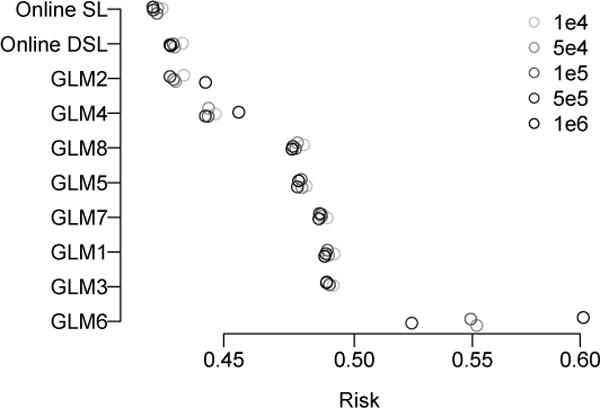
Results from the simulation study. The average risk across 500 simulations is shown for each online algorithm and sample size. Online SL is the online super learner while Online DSL is the online discrete super learner.

6 Online prediction of infectious disease incidence

We used the online super learner to make predictions of disease incidence using data assembled by Project Tycho (van Panhuis et al., 2013). The Project Tycho database is freely available and includes weekly notifiable disease reports for several infectious diseases in the United States. We analyzed the standardized incidence per 100,000 population of Hepatitis A infections. These measures date back to January 1966 and include a total of 90,839 reports. We used the data from years 1966–1968 to generate initial estimates for our candidate online learners and subsequently used the online super learner to make streaming predictions of the weekly standardized incidence of Hepatitis A in each state for each week recorded from 1968–2011. At each week, we based our predictions on the incidence of disease in the previous four weeks. However, many states had at least some missing weekly incidence recordings, so at time t, we used the summary measure Z(t) = {M(t − i), Ÿ(t − i) = M(t − i)Y(t − i): i = 1,…, 4} to generate predictions, where M(i) is the indicator of incidence being recorded at time i. We used the bounded negative log-likelihood loss function to evaluate our predictions,

$$L(\psi )(Y,Z)=-\frac{Y}{u}\mathrm{\text{log}}\left\{\frac{\psi (Z)}{u}\right\}-(1-\frac{Y}{u})\mathrm{\text{log}}\{1-\frac{\psi (Z)}{u}\},$$

where u denotes the upper bound on disease incidence, here set to be 41.6, the maximum observed value. As a simple proof-of-concept, we considered a limited library of candidate online learners consisting of various bounded logistic regression models with parameters estimated via first-order stochastic gradient descent, where we define a bounded logistic regression model as a logistic regression on the transformed outcome Y/u ∈ (0, 1). The regression formulas for the various models are shown in Table 2.

Table 2.

Super learner library for the Tycho data analysis. The formula column shows the regression formula for each bounded logistic regression model used in the analysis. The formula “1” denotes an intercept only model.

Name	Formula
GLM1	1
GLM2	M(t − 1) + Ỹ(t − 1)
GLM3	M(t − 1) + M(t − 2) + Ỹ(t − 1) + Ỹ(t − 2)
GLM4	M(t − 1) + M(t − 2) + M(t − 3) + Ỹ(t − 1) + Ỹ(t − 2) + Ỹ(t − 3)
GLM5	M(t − 1) + M(t − 2) + M(t − 3) + M(t − 4) + Ỹ(t − 1) + Ỹ(t − 2) + Ỹ(t − 3) + Ỹ(t – 4)
GLM6	M(t − 1) + M(t − 2) + Ỹ(t − 1) + Ỹ(t − 2) + I(Ỹ(t − 2) > 0) Ỹ(t − 1)
GLM7	M(t − 1) + M(t − 2) + Ỹ(t − 1) + Ỹ(t − 2) + I(Ỹ(t − 2) > 0)Ỹ(t − 1) + I(Ỹ(t − 3) > 0)~[over]Ỹ(t − 1).
GLM8	M(t − 1) + M(t − 2) + Ỹ(t − 1) + I(Ỹ(t − 2) > 0)
GLM9	M(t − 1) + M(t − 2) + M(t − 3) + Ỹ(t − 1) + I(Ỹ(t − 2) > 0) + I(Ỹ(t − 3) > 0)

We evaluated the performance of the candidate estimators and online super learners based on two criteria: the online cross-validated risk and the risk calculated on a validation set consisting of the final 1,000 recorded weekly reports from 2011–2012, which were withheld from the initial training. The online cross-validated risk is the average loss incurred on weekly predictions made with a given algorithm between 1968 and 2011. The out-of-sample predictive risk is an estimate of the risk of using the predictions from the final models trained using data through 2011 to make predictions of Hepatitis A incidence in the future. The results of the analysis are shown in Figure 2. The online super learner performed the best in terms of online cross-validated risk followed by GLM5 and the discrete online super learner. The discrete online super learner (GLM5) performed best in terms of validation risk followed closely by the online super learner.

Figure 2.

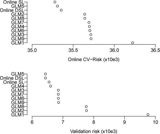
Results for Hepatitis A prediction. The top panel shows the ordered online cross-validated risk of the super learners and candidate online algorithms. The bottom panel shows the ordered risk on the validation data.

7 Discussion

The online super learner can be used for estimation of any common parameter of the conditional probability distribution of O(t), given Ō(t − 1) that minimizes the conditional expectation of a loss function. Our results demonstrate that under weak conditions, this super learner will be asymptotically equivalent with the oracle-selected estimator. These results therefore provide a powerful way to optimally combine multiple estimators in the online, dependent data setting. The results have implications for the case that the statistical target parameter is a pathwise differentiable (typically, low dimensional) parameter of ${\overline{P}}_0$. In this case, an online asymptotically normally distributed, efficient estimator can be constructed using targeted minimum loss-based estimation (van der Laan and Rubin, 2006; van der Laan and Rose, 2011). Such an estimator relies on good initial estimators of certain key nuisance parameters, such as conditional means or densities. The online super learner can therefore be used to aid in construction of online estimators for pathwise differentiable parameters of nonparametric time series models of the type defined in this article.

We expect that the oracle inequality we establish will hold under weaker stationarity assumptions. In particular, depending on the target parameter, the theorem may permit the sole inclusion of stationarity assumptions on relevant portions of the conditional probability distribution of O(t) given Z(t). For example, in the infectious disease prediction problem, our results may allow for the conditional distribution of W(t) given Z(t) to change over time, so long as the conditional distribution of Y(t) given W(t) and Z(t) remains stationary. Confirming this result is left to future work. Also left to future work is implementing the online super learning in a fast, parallelized manner. Such an implementation could ensure that the online super learner requires no more computation time than the slowest candidate online estimator. It will also be important to develop software that incorporates a large library of candidate online estimators, as the performance of the online super learner is limited only by the performance of the best of its constituent online algorithms. The online cross-validation approach could be used to optimally select tuning parameters for a single online algorithm, such as Lasso regression or support vector machines, in an online way. However, as there is unlikely to be a single online algorithm that performs well in every setting and we expect superior performance by considering a large and diverse set of candidate online learners, which might include multiple versions of a single online algorithm, each with different tuning parameters.

An interesting question is whether limiting candidate learners to online learners limits the performance of our procedure relative to an offline super learner that is able to utilize a larger library of offline learners. In situations where it is computationally feasible, there is no reason that not to include offline estimators in the online super learner procedure to study this question directly. These offline estimators would recompute the estimator with each incoming batch of data using the new data and all of the past data. Of course, the online super learner would no longer be an online procedure. Nevertheless, the online cross-validated risk provides an interesting way of comparing online and offline estimators to determine whether there is gain in utilizing computationally intensive offline estimators as opposed to only computationally efficient online estimators. Formally, one could define an algorithm that (1) uses an offline algorithm with each new data point; (2) at each step, checks whether the online cross-validated risk is improved relative to an online version of the estimator; and (3) at the point where the difference in online risk between the offline and online version is small, returns an arbitrary value (e.g., 0). In this way, we guarantee that we are only exerting computational effort to compute the offline estimator so long as it is providing an improvement over the online version. The stopping decision in (3) is pre-specified and based only on past data, so the martingale structure is preserved and our oracle results still apply. The oracle results may extend to more ad-hoc stopping rules that are not defined a-priori; however, we leave the development of the theory around such stopping rules to future work.

References

- Balakrishnan Suhrid, Madigan David. Algorithms for sparse linear classifiers in the massive data setting. Journal of Machine Learning Research. 2008;9:313–337. [Google Scholar]
- Bottou Léon. Proceedings of PCOMPSTAT 2010. Springer; 2010. Large-scale machine learning with stochastic gradient descent; pp. 177–186. [Google Scholar]
- Bousquet Olivier, Bottou Léon. The tradeoffs of large scale learning. Advances in Neural Information Processing Systems. 2008:161–168. doi: 10.1.1.168.5389. [Google Scholar]
- Chambaz A, van der Laan MJ. Targeting the optimal design in randomized clinical trials with binary outcomes and no covariate, theoretical study. International Journal of Biostatistics. 2011a;7(1):1–30. doi: 10.2202/1557-4679.1247. [DOI] [Google Scholar]
- Chambaz A, van der Laan MJ. Targeting the optimal design in randomized clinical trials with binary outcomes and no covariate, simulation study. International Journal of Biostatistics. 2011b;7(1):1–32. doi: 10.2202/1557-4679.1310. [DOI] [Google Scholar]
- Crammer Koby, Dekel Ofer, Keshet Joseph, Shalev Shai-Shwart, Singer Yoram. Online passive-aggressive algorithms. Journal of Machine Learning Research. 2006;7:551–585. [Google Scholar]
- Duchi John, Hazan Elad, Singer Yoram. Adaptive subgradient methods for online learning and stochastic optimization. The Journal of Machine Learning Research. 2011;12:2121–2159. [Google Scholar]
- Fu Wenjiang J. Penalized regressions: The bridge versus the lasso. Journal of Computational and Graphical Statistics. 1998;7(3):397–416. doi: 10.1080/10618600.1998.10474784. [DOI] [Google Scholar]
- Kivinen Jyrki, Smola Alexander J, Williamson Robert C. Online learning with kernels. IEEE Transactions on Signal Processing. 2004;52(8):2165–2176. doi: 10.1109/TSP.2004.830991. [DOI] [Google Scholar]
- Langford John, Li Lihong, Zhang Tong. Sparse online learning via truncated gradient. Journal of Machine Learning Research. 2009 Mar;10:777–801. [Google Scholar]
- Murata Noboru. A statistical study of on-line learning. In: Saad D, editor. Online Learning and Neural Networks. Cambridge University Press; Cambridge, UK: 1999. [Google Scholar]
- Pirracchio Romain, Petersen Maya L, Carone Marco, Resche Rigon Matthieu, Chevret Sylvie, van der Laan Mark J. Mortality prediction in intensive care units with the Super ICU Learner Algorithm (SICULA): A population-based study. The Lancet Respiratory Medicine. 2015;3(1):42–52. doi: 10.1016/S2213-26001470239-5. [DOI] [PMC free article] [PubMed] [Google Scholar]
- Polyak Boris T, Juditsky Anatoli B. Acceleration of stochastic approximation by averaging. SIAM Journal on Control and Optimization. 1992;30(4):838–855. doi: 10.1137/0330046. [DOI] [Google Scholar]
- Rose Sherri. Mortality risk score prediction in an elderly population using machine learning. American Journal of Epidemiology. 2013;177(5):443–452. doi: 10.1093/aje/kws241. [DOI] [PubMed] [Google Scholar]
- Shalev-Shwartz Shai. Online learning and online convex optimization. Foundations and Trends in Machine Learning. 2011;4(2):107–194. doi: 10.1561/2200000018. [DOI] [Google Scholar]
- Shalev-Shwartz Shai, Singer Yoram, Srebro Nathan, Cotter Andrew. Pegasos: Primal estimated sub-gradient solver for svm. Mathematical Programming. 2011;127(1):3–30. doi: 10.1007/s10107-010-0420-4. [DOI] [Google Scholar]
- van der Laan MJ, Dudoit S. Technical Report 130. Division of Biostatistics, University of California; Berkeley: 2003. Unified cross-validation methodology for selection among estimators and a general cross-validated adaptive epsilonnet estimator: finite sample oracle inequalities and examples. [Google Scholar]
- van der Laan MJ, Rose S. Targeted Learning: Causal Inference for Observational and Experimental Data. Springer; Berlin Heidelberg New York: 2011. [DOI] [Google Scholar]
- van der Laan MJ, Rubin Daniel B. Targeted maximum likelihood learning. International Journal of Biostatistics. 2006;2(1) doi: 10.2202/1557-4679.1043. Article 11. [DOI] [Google Scholar]
- van der Laan MJ, Dudoit S, van der Vaart AW. The cross-validated adaptive epsilon-net estimator. Stat Decis. 2006;24(3):373–395. doi: 10.1524/stnd.2006.24.3.373. [DOI] [Google Scholar]
- van der Laan MJ, Polley EC, Hubbard AE. Super learner. Statistical Applications in Genetics and Molecular Biology. 2007;6(1) doi: 10.2202/1544-6115.1309. [DOI] [PubMed] [Google Scholar]
- van der Vaart AW, Dudoit S, van der Laan MJ. Oracle inequalities for multi-fold cross-validation. Stat Decis. 2006;24(3):351–371. doi: 10.1524/stnd.2006.24.3.351. [DOI] [Google Scholar]
- van Panhuis Willem G, Grefenstette John, Jung Su Yon, Shong Chok Nian, Cross Anne, Eng Heather, Lee Bruce Y, Zadorozhny Vladimir, Brown Shawn, Cummings Derek, et al. Contagious diseases in the United States from 1888 to the present. The New England Journal of Medicine. 2013;369(22):2152. doi: 10.1056/NEJMms1215400. [DOI] [PMC free article] [PubMed] [Google Scholar]
- Xu Wei. Towards optimal one pass large scale learning with averaged stochastic gradient descent. 2011 arXiv preprint arXiv:1107.2490. [Google Scholar]
- Zeiler Matthew D. ADADELTA: An adaptive learning rate method. 2012 arXiv preprint arXiv:1212.5701. [Google Scholar]
- Zinkevich Martin. Online convex programming and generalized infinitesimal gradient ascent. Proceedings of the Twentieth International Conference on Machine Learning. 2003 [Google Scholar]
Associated Data
This section collects any data citations, data availability statements, or supplementary materials included in this article.