WHATCH’EM: A Weather-Driven Energy Balance Model for Determining Water Height and Temperature in Container Habitats for Aedes aegypti

Abstract

The mosquito virus vector Aedes (Ae.) aegypti exploits a wide range of containers as sites for egg laying and development of the immature life stages, yet the approaches for modeling meteorologically sensitive container water dynamics have been limited. This study introduces the Water Height and Temperature in Container Habitats Energy Model (WHATCH’EM), a state-of-the-science, physically based energy balance model of water height and temperature in containers that may serve as development sites for mosquitoes. The authors employ WHATCH’EM to model container water dynamics in three cities along a climatic gradient in México ranging from sea level, where Ae. aegypti is highly abundant, to ~2100 m, where Ae. aegypti is rarely found. When compared with measurements from a 1-month field experiment in two of these cities during summer 2013, WHATCH’EM realistically simulates the daily mean and range of water temperature for a variety of containers. To examine container dynamics for an entire season, WHATCH’EM is also driven with field-derived meteorological data from May to September 2011 and evaluated for three commonly encountered container types. WHATCH’EM simulates the highly nonlinear manner in which air temperature, humidity, rainfall, clouds, and container characteristics (shape, size, and color) determine water temperature and height. Sunlight exposure, modulated by clouds and shading from nearby objects, plays a first-order role. In general, simulated water temperatures are higher for containers that are larger, darker, and receive more sunlight. WHATCH’EM simulations will be helpful in understanding the limiting meteorological and container-related factors for proliferation of Ae. aegypti and may be useful for informing weather-driven early warning systems for viruses transmitted by Ae. aegypti.

1. Introduction

The mosquito Aedes (Ae.) aegypti, the primary vector of dengue, yellow fever, and chikungunya viruses, exploits a wide range of containers as sites for egg laying and development of the immature (larval and pupal) life stages (Gratz 1999, 2004; Gubler 2004; Focks and Alexander 2006). These containers can range in size from small trash items (e.g., bottles and cans) to medium-sized buckets and tires to large water storage containers such as barrels, tanks, and cisterns (Morrison et al. 2004; Tun-Lin et al. 2009; Bartlett-Healy et al. 2012; Hiscox et al. 2013). Proliferation of the mosquitoes is aided by the presence of containers that hold water of suitable temperature and nutrient content for eggs to hatch and immatures to develop. Successful larval development of Ae. aegypti can be impeded by water temperatures that are too low for development to occur (8°–12°C) or high enough to cause physical harm, through heat stress, to the larvae (36°–44°C) (Bar-Zeev 1958; Smith et al. 1988; Tun-Lin et al. 2000; Kamimura et al. 2002; Chang et al. 2007; Richardson et al. 2011; Muturi et al. 2012). In the field, Hemme et al. (2009) found that Ae. aegypti immatures were absent from water storage drums, which are key productive containers in Trinidad, when water temperatures exceeded 32°C. The temperature optimum for Ae. aegypti larval and pupal development, with short development times and high survival rates, is in the range of 24°–34°C (Bar-Zeev 1958; Rueda et al. 1990; Tun-Lin et al. 2000; Kamimura et al. 2002; Mohammed and Chadee 2011; Padmanabha et al. 2011b, 2012; Richardson et al. 2011; Farjana et al. 2012; Eisen et al. 2014). There also is a growing recognition that the magnitude of the daily temperature range (i.e., fluctuations over the course of a 24-h period) impact life history traits of Ae. aegypti, including larval development time (Lambrechts et al. 2011; Mohammed and Chadee 2011; Carrington et al. 2013a, b). Other factors that can have negative effects on larval development time or survival include poor nutrient content of the water and intraspecific or interspecific resource competition (Braks et al. 2004; Juliano et al. 2004; Padmanabha et al. 2011a; Walsh et al. 2011; Couret et al. 2014; Levi et al. 2014). For rain-filled containers, there are also distinct risks of a container drying out before the immature stages can complete their development or of the container overflowing and the immatures being flushed out (Koenraadt and Harrington 2008; Bartlett-Healy et al. 2011).

Weather-driven simulation models for Ae. aegypti populations—such as Container Inhabiting Mosquito Simulation Model (CIMSiM) and Skeeter Buster—are strongly influenced by both air and water temperature, the latter of which impacts several important components of the models including the development times and survival rates of eggs, larvae, and pupae (Focks et al. 1993a,b; Cheng et al. 1998; Magori et al. 2009; Ellis et al. 2011). Water temperature and volume dynamics in potential container habitats are complex (Richardson et al. 2013), yet perhaps the greatest limitation of the weather-driven Ae. aegypti simulation models is the continued use of simplistic empirical relationships to predict water temperature in and water loss from containers based on ambient air temperature (daily maximum and minimum), sunlight exposure, precipitation, relative humidity, and saturation deficit (Focks et al. 1993a; Cheng et al. 1998). Recent work has shown that physics-based approaches toward modeling container water properties are promising for resolving the complexities of container water dynamics (Tarakidzwa 1997; Kearney et al. 2009).

In the present study, we introduce a new state-of-the-science, physically based model, as opposed to an empirical approach, to explore water dynamics in container habitats of relevance for Ae. aegypti. The model calculates the height and temperature of water in a specified container at user-specified intervals by solving the system of equations that governs the energy balance (i.e., heat and moisture budget) of the container as a function of meteorological and user-prescribed inputs. The model is therefore distinct from the energy budget model presented by Kearney et al. (2009) in that it simulates container water dynamics at user-specified time scales, whereas Kearney et al. addressed monthly time scales. The current approach 1) accounts for the highly nonlinear manner in which air temperature, humidity, rainfall, and clouds or shading interact with a specified container at subdaily time scales to determine the height and temperature of the water it contains and 2) facilitates integration into weather-driven mosquito life cycle modeling frameworks that operate on daily time scales, such as CIMSiM and Skeeter Buster. The model, henceforth called the Water Height and Temperature in Container Habitats Energy Model (WHATCH’EM) is designed to be driven by readily available meteorological observations and user-specifiable container characteristics, so that it can be easily applied by a variety of users.

A field study was conducted to determine the abundance of Ae. aegypti immatures in containers in 12 communities located along an elevation and climate gradient in central México (Lozano-Fuentes et al. 2012, 2014). Three representative communities along this gradient are Veracruz City at sea level, with highly favorable climatic conditions for the mosquito; Rio Blanco along the eastern slopes of the Sierra Madre Oriental (~1250 m), where the mosquito is moderately abundant; and Puebla City in the central highlands (~2100 m), where a few specimens of Ae. aegypti were encountered, but the climate appears to prevent the mosquito from proliferating. Mosquito abundance is strongly correlated with weather variables along this gradient, including positive correlations with average minimum daily ambient air temperature, average daily minimum relative humidity, and total rainfall and negative correlations with daily ambient air temperature range during the 30-day period preceding the mosquito survey in a given community (Lozano-Fuentes et al. 2012). These findings led us to speculate that low or greatly fluctuating water temperatures in containers may be limiting factors for population buildup of Ae. aegypti at the higher elevations. Therefore, we apply WHATCH’EM to explore water dynamics in three commonly encountered container types—small buckets (3.8 L), medium-sized buckets (18.9 L), and large drums (120–208.2 L)—at the three cities noted above. First, we validate WHATCH’EM in two of the cities, Veracruz City and Rio Blanco, by comparing WHATCH’EM simulations for the three container types to water temperature and height measurements from a 1-month field experiment conducted in summer 2013 and to output from the Cheng et al. (1998) model that is similar to the methods used for water temperature calculations in CIMSiM and Skeeter Buster. Next, a series of sensitivity simulations from WHATCH’EM is used to examine the impacts of shading, clouds, and container color on the simulated water height and temperature in the three container types and three locations throughout an entire season. The model is driven by meteorological observations taken in each city during our initial field season from May to September 2011, the time of year during which environmental conditions are best suited (i.e., with combined high temperature and substantial rainfall) for the proliferation of Ae. aegypti in the study area.

2. Methods

2.1. WHATCH’EM model description

WHATCH’EM simulates the water height (analogous with water volume) and water temperature of a specified container, based on the energy balance of the water and the container. The full model documentation and source code can be obtained from Steinhoff and Monaghan (2013).

The energy balance method is used to calculate heat and moisture exchanges between the surface and atmosphere in numerical weather prediction models in order to estimate the surface temperature and evaporation. A similar method is used here, adjusted for container geometries and thermodynamic characteristics. WHATCH’EM requires as input a minimal amount of commonly available meteorological data (temperature, relative humidity, and rainfall) to produce water temperature and level estimates. Optional radiation, cloud, soil, and wind data can be used to improve the realism of simulations. WHATCH’EM takes into account variable factors such as cloudiness, shading, container size, and thermal characteristics and any manual container filling that may occur. WHATCH’EM can model rectangular containers, round containers, and tires. Lids and tilted containers (i.e., containers not fully resting on the ground surface) can be accounted for. The energy balance is calculated for both the water and the container. The energy balance for water is based on the following equation:

$$Q_{\text{STW}}=Q_{\text{SW}\downarrow }+Q_{\text{LW}\downarrow }-Q_{\text{LW}\uparrow }-Q_{H\uparrow }-Q_{L\uparrow }-Q_{C\downarrow }-Q_{C\to },$$ (1)

where Q_STW is heat storage in water (representing the change of temperature of the water), Q_SW↓ is net shortwave (SW) radiation, Q_LW↓ is downward longwave (LW) radiation, Q_LW↑ is upward longwave radiation, Q_H↑ is sensible heat (SH) transfer, Q_L↑ is latent heat transfer (LH), Q_C↓ is conduction between the water and container bottom, and Q_C→ is conduction between the water and container sidewalls. The energy balance for the container is

$$Q_{\text{STC}}=Q_{\text{SW}\to }+Q_{\text{LW}\to }-Q_{\text{LW}\leftarrow }-Q_{H\leftarrow }-Q_{G\downarrow }+Q_{C\downarrow }+Q_{C\to },$$ (2)

where Q_STC is heat storage in the container, Q_SW→ is sideways inbound shortwave radiation, Q_LW→ is sideways inbound longwave radiation, Q_LW←is sideways outbound longwave radiation, Q_H←is sideways sensible heat transfer, Q_G↓ is conduction between the ground and the container bottom, and Q_C↓ and Q_C→ are the same as in (1). Figure 1 is a schematic showing the terms in (1) and (2) relative to the water and container. All terms are in units of power (watts), and the sign convention is that all radiation terms are positive into the container or its water; sensible, latent, and ground fluxes are positive out of the container or its water; and conduction terms are positive into the container.

Figure 1.

Schematic showing terms of energy balance model introduced in (1) and (2). Terms are described in the text.

The downward solar radiation Q_SW↓ is absorbed by the water through the top opening of the container. The shortwave radiation absorbed into the water is that component not reflected by water or blocked by shade or clouds; Q_SW↓ is calculated as

$$Q_{\text{SW}\downarrow }=S_t{A}_t(1-a_w)(1-\beta )(1-d_v)-Q_i,$$ (3)

where S_t is the total downward shortwave radiative flux (based on solar zenith angle at the user-specified coordinates for the site of interest, and the transmission of solar radiation through the atmosphere, which is a function of cloud cover), A_t is container top opening area, a_w is the reflectivity (albedo) coefficient of water [a function of the solar zenith angle per Cogley (1979)], β is the shade fraction, d_υ is the fraction deviation of the top opening of the container from vertical, and Q_i is the solar radiation absorbed by the inside container walls when the container is not 100% full (accounted for in Q_b below).

The sideways inbound solar radiation Q_SW→ is absorbed by the container sidewalls. It is composed of two components—solar radiation directly striking the container sidewalls and diffuse solar radiation—not reflected by the container. As given below Q_SW→ is calculated as

$$Q_{\text{SW}\to }=(1-a_c)(Q_b+Q_d),$$ (4)

where a_c is the reflectivity coefficient of the container, Q_b is the direct component (accounting for the zenith angle of the sun and absorption on interior sidewalls), and the diffuse component Q_d is a combination of solar radiation reflected from the ground onto the container sidewalls and atmospheric scattering. Similar to (3), the Q_b and Q_d terms take into account the surface area of the container and shading effects.

The downward longwave radiation Q_LW↓ is absorbed by water through the top opening of the container, emitted by the atmosphere, clouds, and any shading surface. The emitted longwave radiation is dependent on the fourth power of temperature (through the Stefan–Boltzmann law) and properties of the emitting body. Below Q_LW↓ is calculated as

$$Q_{\text{LW}\downarrow }=A_t[(1-\beta ){\epsilon }_a\sigma T_a^4+\beta {\epsilon }_s\sigma T_s^4],$$ (5)

where ε_a is emissivity of the atmosphere [itself a time-variable function of air temperature, vapor pressure, and cloud fraction per Prata (1996) and Crawford and Duchon (1999)], σ is the Stefan–Boltzmann constant, ε_s is emissivity of the shading surface, and T_s is the temperature of the shading surface (assumed equal to the air temperature T_a).

The upward longwave radiation Q_LW↑ is emitted by water in the container into the atmosphere above. It depends on the temperature and emitting properties of water. Here Q_LW↑ is calculated as

$$Q_{\text{LW}\uparrow }=A_t{\epsilon }_w\sigma T_w^4,$$ (6)

where ε_w is emissivity of water, and T_w is water temperature.

The sideways inbound longwave radiation Q_LW→ is absorbed by the container sidewalls, assumed to be split equally between longwave radiation emitted by the atmosphere and by the ground. It is calculated as

$$Q_{\text{LW}\to }=A_s(0.5{\epsilon }_g\sigma T_g^4+0.5{\epsilon }_a\sigma T_a^4),$$ (7)

where A_s is surface area of the container sidewalls (taking into account any deviation of the top opening from vertical), ε_g is emissivity of the ground surface, and T_g is the ground temperature.

The sideways outbound longwave radiation Q_LW←is emitted by the container sidewalls to the surrounding air and ground. It is calculated as

$$Q_{\text{LW}\leftarrow }=A_s{\epsilon }_c\sigma T_c^4,$$ (8)

where ε_c is emissivity of the container, and T_c is the temperature of the container.

The sensible heat transfer Q_H↑ is between the water in the container and the air above. Calculations of sensible heat transfer are dependent upon the convective regime (forced, free, or mixed) and the associated nondimensional groups of quantities, which the model takes into account. The calculation for Q_H↑ is from Monteith and Unsworth (2008, p. 161):

$$Q_{H\uparrow }=\frac{A_t{C}_a(T_w-T_a)}{r_H},$$ (9)

where C_a is the heat capacity of air, and r_H is heat transfer resistance, itself a time-variable function of the Nusselt number (Steinhoff and Monaghan 2013). The sensible heat transfer Q_H←is between the container and surrounding air. It is calculated similar to (9), except that it is computed based on the surface area and temperature of the container sides, and r_H employs a different Nusselt number representing the geometry of the container sides:

$$Q_{H\leftarrow }=\frac{A_s{C}_a(T_c-T_a)}{r_H}.$$ (10)

The latent heat transfer Q_L↑ is associated with phase changes of water. Specifically for this application, it is the heat supplied to vaporization of water in the container to the air above, and represents a heat sink for the water in the container. It is calculated from

$$Q_{L\uparrow }=\frac{A_t\lambda (e_s-e)}{r_W},$$ (11)

where e_s is saturation vapor pressure, e is vapor pressure, λ is the latent heat of vaporization, and r_W is the water vapor transfer resistance, calculated in a similar manner to r_H (Monteith and Unsworth 2008).

The heat conduction Q_G↓ between the bottom of the container and the underlying soil depends primarily on calculation of the temperature gradient between the soil and the container:

$$Q_{G\downarrow }=\frac{A_b(T_c-T_g)}{\sum \left(\frac{\mathrm{\Delta }z}{k}\right)},$$ (12)

where A_b is the container bottom area, Δz is the differential layer depth, and k is thermal conductivity. The ratio of the last two terms is summed for half of the thickness of the ground layer (z_g, k_g) and half of the thickness of the container (z_c, k_c), under the assumption that T_c and T_g occur at the middle of each volume. The default value of z_g is 50 mm because it is the midpoint of the 0–100-mm upper soil layer for which temperature data are commonly available in atmospheric re-analysis products.

The heat conduction Q_C↓ between the water and the bottom of the container is specified as

$$Q_{C\downarrow }=\frac{A_b(T_w-T_c)}{\sum \left(\frac{\mathrm{\Delta }z}{k}\right)},$$ (13)

where notations are as before, with the ratio of the last two terms summed for half of the thickness of the container and half of the depth of the water. Similarly, Q_C→ is the heat conduction between the water and the sides of the container:

$$Q_{C\to }=\frac{A_s(T_w-T_c)}{\sum \left(\frac{\mathrm{\Delta }z}{k}\right)},$$ (14)

with the ratio of the last two terms summed for half of the thickness of the container and the half the diameter (i.e., the radius) of the water.

Once the heat storage terms Q_STW and Q_STC have been calculated using the water container energy balance equations (1) and (2), the water height in the container and the water and container temperatures are updated. First, the accumulated evaporation of water from the container is calculated from the latent heat transfer Q_L↑, following Monteith and Unsworth (2008, p. 255):

$$E=\frac{Q_{L\uparrow }\mathrm{\Delta }t}{A_t\lambda {\rho }_w},$$ (15)

where Δt is the time period of the accumulated evaporation, and ρ_w is the density of water. The water height change is then calculated based on the difference of evaporation and precipitation over the time period Δt:

$$\mathrm{\Delta }{h}_w=P(1-\beta )(A_t/A_b)+\text{MF}-E,$$ (16)

where Δh_w is the water height change, P is precipitation accumulated over the time period Δt, the ratio A_t /A_b accounts for the amount of rainfall that can enter through the container top relative to the size of the container body (i.e., if the diameters of the top container opening and the body of the container are different), and MF is any manual fill. Currently, the minimum water height allowed in the program, for numerical stability reasons, is 15 mm. Below this, water temperature and all energy balance terms are set to a missing value, and a constant evaporation rate is set (default is 0.02 mm h⁻¹). If, through precipitation or manual filling, water height returns above 15 mm, then calculations are restarted with water temperature set to the initial water temperature specified at the beginning of the simulation. It is noteworthy that while the abundance of Ae. aegypti immatures is positively correlated with water volume, some immatures can survive in small volumes of water having heights less than 15 mm, such as in water that pools on plastic tarps (Barrera et al. 2006); thus, a current limitation of WHATCH’EM is that it does not resolve these situations in which very little water is present.

With updated water height, the change to the temperature of the water in the container is calculated as

$$\mathrm{\Delta }{T}_w=\frac{Q_{\text{STW}}\mathrm{\Delta }t}{A_t{h}_w{C}_w},$$ (17)

where ΔT_w is the water temperature change, h_w is the updated water height (note that A_th_w is the water volume), and C_w is the heat capacity of water. Similarly, the container temperature is calculated as

$$\mathrm{\Delta }{T}_c=\frac{Q_{\text{STC}}\mathrm{\Delta }t}{V_c{C}_c},$$ (18)

where ΔT_c is the container temperature change, V_c is the volume of the container material, and C_c is the heat capacity of the container material.

Because the calculations of water and container temperature changes involve the terms themselves and form a series of ordinary differential equations, numerical methods are used to simultaneously solve the equation system. In WHATCH’EM, the fourth-order Adams–Moulton (AM) predictor–corrector method is used, which is started with a fourth-order Runge–Kutta (RK) procedure (e.g., Cheney and Kincaid 2007). The RK procedure is a single time-step process and is needed at the beginning of the simulation since the AM procedure requires multiple time steps.

2.2. Data and simulation descriptions

2.2.1. Meteorological data

There are three required meteorological variables, and several optional variables, for input to WHATCH’EM at hourly intervals. The required variables are air temperature (°C), relative humidity (%), and rainfall (mm h⁻¹). For this study, temperature and relative humidity were obtained from HOBO dataloggers (Onset Computer Corporation, Bourne, Massachusetts) installed in Veracruz City, Rio Blanco, and Puebla City. For a map showing the locations of these cities in Veracruz and Puebla States, México, see Lozano-Fuentes et al. (2012). Rainfall data were obtained from Stratus RG202 rain gauge (Productive Alternatives, Inc., Fergus Falls, Minnesota) for the validation experiments and from the 0.07° gridded Climate Prediction Center morphing technique (CMORPH) dataset (Joyce et al. 2004) for the sensitivity experiments. CMORPH uses precipitation estimates derived exclusively from low orbiter satellite microwave observations and features transported via spatial propagation of information obtained from geostationary satellite infrared imagery. CMORPH provides some of the most reliable estimates for tropical summer rainfall compared to other satellite- and model-based rainfall products (Ebert et al. 2007). CMORPH data, which cover the globe from 60°S to 60°N, were bilinearly interpolated from the four surrounding grid points to each HOBO site.

Optional variables include either downward incident shortwave and longwave radiation or cloud fraction (low, middle, and high), soil temperature (°C), wind speed (m s⁻¹), and surface pressure (hPa). For this application, all optional variables (using radiation terms instead of cloud fraction) are obtained from the Global Land Data Assimilation System (GLDAS; Rodell et al. 2004), which utilizes satellite- and ground-based observations and the Land Information System (LIS; Kumar et al. 2006) to run a suite of offline land surface models for optimal estimation of ground surface and soil conditions. GLDAS, version 1, output is available at 0.25° grid spacing globally north of 60°S at 3-hourly intervals (a 15-min model time step is used) for 2000–present near–real time, with output utilizing the four layer National Centers for Environmental Prediction–Oregon State University–Air Force–Hydrologic Research Laboratory (Noah) land surface model (Chen et al. 1996; Koren et al. 1999).

If radiation data are unavailable, cloud fraction data can be input, and estimates of downward radiation terms will be calculated. If cloud fraction data are not provided, then low, middle, and high cloud fraction estimates are user specified for both daytime and nighttime conditions. If soil temperature data are unavailable, a constant value must be specified. If wind speed and/or surface pressure data are unavailable, constant values can be specified.

2.2.2. Average weather conditions

The average weather conditions of Veracruz City, Rio Blanco, and Puebla City for May–September 2011 are compared in Figure 2. Monthly and total average temperatures (Figure 2a) follow the elevation gradient between the cities, with Veracruz City, near sea level, being the warmest overall (29.0°C for the May–September average), followed by Rio Blanco (~1250 m above sea level; 21.3°C) and Puebla City (~2100 m; 18.5°C). The average daily temperature range (Figure 2b) increases markedly along the elevation gradient, being much lower in Veracruz City (3.9°C) versus the higher elevation environments of Rio Blanco (9.0°C) and Puebla City (10.9°C). In contrast, relative humidity does not exhibit marked variability between the cities during the May–September period (Figure 2c). In fact, the highest average relative humidity occurs in Rio Blanco, where temperatures are cooler than in Veracruz City, but the influence of humid air from the Gulf of Mexico is still strong. However, the specific humidity (a measure of absolute humidity that is independent of temperature) clearly shows that Veracruz City is more humid than Rio Blanco and that Puebla City is the least humid of all the cities (Figure 2d). Likewise, the highest overall rainfall totals and cloud amounts occur in Veracruz City (although the onset of rains is later there), followed by Rio Blanco and Puebla City, which have similar rainfall totals and cloud amounts (Figures 2e,f). In summary, during May–September Veracruz City is comparatively warm and humid with a small daily temperature range and the greatest rainfall, whereas Puebla City is comparatively cool and arid with a large daily temperature range and lower rainfall. Rio Blanco’s climate is intermediate between Veracruz City and Puebla City.

Figure 2.

Monthly data for selected climate variables for Veracruz City (red), Rio Blanco (green), and Puebla City (blue) during May–September 2011. The All column is the seasonal average or total over all months.

2.2.3. Approach for WHATCH’EM validation

To provide validation for container water temperature and height estimates from WHATCH’EM, a series of container experiments were performed on satellite campuses of Universidad Veracruzana in Boca del Rio (19.1°N, 96.1°W) and Orizaba (19.0°N, 97.3°W) for a ~1-month period spanning 3 June 2013 through 4 July 2013. Because Boca del Rio is adjacent to Veracruz City, and Orizaba is adjacent to Rio Blanco, for consistency with our sensitivity simulations (described below) we refer to these two sites as Veracruz City and Rio Blanco, respectively. At each site, three sets of four different containers (3.8-L small black bucket, 18.9-L medium black and white buckets, and 120-L large gray trash cans) were set up in different shading regimes (no shade, partial shade, and full shade; e.g., Figure 3a). We chose these particular container types because they are representative of containers commonly encountered in the field (Lozano-Fuentes et al. 2012). Here, partial shade represents fractional continuous shading, as opposed to the shading fraction varying throughout the day. Water was initially filled to 75% of the container height and changes in water height were recorded daily and water height reestablished to 75% after measurement, with evaporation calculated after accounting for rainfall recorded by the rain gauge. Water added to the container to reestablish 75% height was taken from a reservoir exposed to ambient weather conditions. Water temperature sensors were suspended in the middle of the water volume of each container using fishing line and weights, and temperature was automatically recorded every 15 min (Figure 3b). Air temperature and relative humidity measurements were also recorded at each site with the HOBO loggers described above.

Figure 3.

The containers used in the WHATCH’EM simulations: (a) no shade validation experiment at the site near Rio Blanco showing the small container at far left (3.8 L; 175 mm width × 185 mm height), the medium container at center (18.9 L; 286 mm width × 350 mm height), and large trash container at far right (120 L; 490 mm width × 685 mm height). (b) Closeup showing temperature sensor in a medium-sized container. (c) The large drum container used for the sensitivity simulations (208.2 L; 597 mm width × 921 mm height) (note that blue is not the color assumed for the simulations). Additional container information can be found in Table 1. Photos are courtesy of D. Steinhoff and A. Monaghan.

WHATCH’EM simulations were performed for each container and shading scenario described above for both field sites, initialized at 0000 coordinated universal time (UTC) on 3 June 2013 and run through 0000 UTC 5 July 2013. The WHATCH’EM configuration and parameters were similar to what is described below for the sensitivity simulations, with the exception that rainfall input was from the rain gauge observations, the ground surface type under the containers was set to match what was observed in the field (i.e., concrete, grass, and bare soil), and the largest container was 120 L (a large trash can) rather than 208.2 L (a 55-gallon drum) due to logistics and availability. Coinciding with the daily manual filling to 75% container height, water height in WHATCH’EM is also reestablished to 75% height at the same time. WHATCH’EM outputs used for the validation included hourly water temperature and evaporation minus precipitation (E − P), which were then averaged for maximum and minimum temperature and E − P for 3 June–4 July 2013.

Estimates of water temperature were also calculated using the empirical equations from Cheng et al. (1998) for maximum and minimum daily container water temperatures. Maximum water temperature is a function of maximum air temperature, minimum dewpoint temperature, and sunlight exposure. Minimum water temperature is a function of minimum air temperature, maximum dewpoint temperature, and a shelter factor that accounts for longwave radiation exchanges with nearby objects. Maximum and minimum air and dewpoint temperature values were calculated from the HOBO temperature and humidity measurements taken at each site. The sunlight exposure factors were set to 1.0, 0.55, and 0.05 for the no shade, partial shade, and full shade experiments, respectively, which is approximately equivalent to one minus the value for the shading factor used for the WHATCH’EM simulations for each experiment. The shelter factors were set to 0.0 for the no shade experiment and 0.1 for the partial and full shade experiments, consistent with the values used by Cheng et al. (1998) for the no shade, under a tree, and under a shed roof with no walls cases. The shelter factors used by Cheng et al. (1998) varied from 0.0 to 0.2, so the values chosen here for the comparison are appropriate based on our shading scenarios and proximity to objects that emit radiation. Cheng et al. (1998), following Focks et al. (1993a), specify that for their equations water temperatures for containers with capacities between 5 and 100 L are averaged over 2 days, and those with capacities between 100 and 500 L are averaged over 3 days. Therefore, for the Cheng et al. (1998) water temperature calculations, we averaged the medium container results over 2 days, and the large container results over 3 days.

2.2.4. Approach for WHATCH’EM sensitivity experiments

WHATCH’EM sensitivity simulations were performed for Veracruz City (19.2°N, 96.1°W), Rio Blanco (18.8°N, 97.2°W), and Puebla City (19.0°N, 98.2°W) for three sets of experimental conditions during the entire May–September 2011 field season. First, we used three container types: small buckets (3.8 L, 1 gallon), medium-sized buckets (18.9 L, 5 gallons), and large drums (208.2 L, 55 gallons; Figures 3a,c). For each container type, the height, radius, thickness, and thermal conductivity is user specified to WHATCH’EM. Second, we evaluated three colors for the containers: black, gray, and white, corresponding to container albedos a_c of 0.1, 0.5, and 0.9, respectively. Container albedo (reflectivity) and thermal conductivity values are estimated online (from www.engineeringtoolbox.com). Third, we examined three levels of shade: no shade, half shade, and full shade. Shade from natural objects (e.g., trees) or human-made structures (e.g., walls or roofs) affect both the longwave and shortwave energy balance and the precipitation received.

The simulations were run for two different scenarios with regards to containers being filled with water: 1) with weekly manual container filling enabled (i.e., the containers are topped off by human action every 168 h) and 2) with manual filling disabled (i.e., the containers only receive water through rainfall). For each of these scenarios, the full set of combinations of the three experimental conditions described above was performed, such that there are 3 × 3 × 3 = 27 total experiments per scenario. The simulations were initialized for 0000 UTC 1 May 2011 because May is near the end of the dry season in the study area but still precedes the onset of the rainy season (in June or July) when Ae. aegypti populations are expected to begin increasing. For the scenario in which there is no manual filling, the containers are assumed to be dry at initialization on 1 May, after months of little or no rainfall. Initial values for water temperature are also user specified for the simulations with manual filling since the containers are full from the onset. WHATCH’EM is integrated once per minute from the initial time point through 0000 UTC on 15 September 2011 in our simulations. This is an arbitrarily chosen time point that likely represents the latter part of the active season for Ae. aegypti at the highest elevation examined, where the climate in the winter is cold enough to prevent activity by this mosquito. Table 1 lists the values of the constants and parameters that are used in WHATCH’EM.

Table 1.

List of constants and parameters used in the WHATCH’EM model.

Parameter	Name	Units	Value
			3.8 L	18.9 L	208.2 L
aw	Albedo of water	Fraction (0–1)		Cogley (1979)
ac	Albedo of container	Fraction (0–1)		0.1, 0.5, 0.9a
β	Shade fraction	Fraction (0–1)		0.0, 0.5, 1.0b
Ca	Heat capacity of air	J m−3 K−1		1230
Cw	Heat capacity of water	J m−3 K−1		4.31 × 106
Cc	Heat capacity of container	J m−3 K−1	2.20 × 106	2.20 × 106	2.20 × 106
εa	Emissivity of atmosphere	Fraction (0–1)		Prata (1996)
εc	Emissivity of container	Fraction (0–1)		0.95
εg	Emissivity of ground surface	Fraction (0–1)		0.95
εs	Emissivity of shading surface	Fraction (0–1)		0.90
εw	Emissivity of water	Fraction (0–1)		0.95
kc	Thermal conductivity of container	W m−1 K−1	0.30	0.50	0.50
kg	Thermal conductivity of groundc	W m−1 K−1		0.92
kw	Thermal conductivity of water	W m−1 K−1		0.57
ρw	Density of water	kg m−3	1025
rH	Heat transfer resistance	s m−1	Monteith and Unsworth (2008)
rW	Water vapor transfer resistance	s m−1	Monteith and Unsworth (2008)
σ	Stefan–Boltzmann constant	W m−2 K−4		5.67 × 10−8
λ	Latent heat of vaporization	J kg−1		2.45 × 106
zc	Thickness of container	m	0.001	0.002	0.002
zg	Thickness of ground layer under container	m		0.05

^aThree different values used for black, gray, and white container experiments, respectively.

^bThree different values used for no shade, half shade, and full shade experiments, respectively.

^cSoil is assumed to be clay, 50% saturated.

3. Results

3.1. Validation of WHATCH’EM

Figure 4 shows time series plots of water temperature from observations and WHATCH’EM simulations over the 3 June–4 July 2013 experiment period for Veracruz (Figure 4a) and Rio Blanco (Figure 4b) with medium black containers in partial shade. WHATCH’EM tracks the diurnal and synoptic-scale variations in water temperature at both sites, with negative biases at Veracruz, negative biases for the warmest daytime conditions, and positive nighttime biases for Rio Blanco. These biases hold for other container sizes and colors and other shading scenarios (not shown).

Figure 4.

Time series comparison of water temperature (°C) from observations (red) and WHATCH’EM simulations (green) for (a) Veracruz and (b) Rio Blanco for the 3 Jun–4 Jul 2013 experiment period.

Basic validation statistics for WHATCH’EM against experiment observations are shown for Veracruz and Rio Blanco in Tables 2 and 3, respectively. For Veracruz, there are only small systematic errors (biases), with larger RMSE values for no shade and partial shade conditions that are likely errors in cloud cover and shortwave radiation. Temporal correlation between WHATCH’EM and observations exceeds 0.87 for no shade and full shade conditions, whereas lower correlation values are found for partial shade conditions because of the shortwave radiation discrepancies around sunrise and sunset. For Rio Blanco, WHATCH’EM is systematically too warm, with additional cloud cover discrepancies that are of similar magnitude as found for Veracruz (represented by the differences between bias and RMSE values). Correlation values for Rio Blanco are similar to Veracruz, with slightly lower values for no shade and full shade conditions and generally larger values for partial shade.

Table 2.

Bias, RMSE, and correlation of WHATCH’EM container water temperature against observations for Veracruz. Bias and RMSE units in °C.

Bias
Container	No shade	Partial shade	Full shade
Small	−0.25	0.06	−0.10
Medium Black	−0.64	0.00	−0.26
Medium White	−0.44	0.02	−0.32
Large	−0.62	−0.08	−0.48
RMSE
Container	No shade	Partial shade	Full shade
Small	2.05	3.16	0.58
Medium black	1.79	1.85	0.55
Medium white	2.10	1.74	0.59
Large	1.77	1.20	0.63
Correlation
Container	No shade	Partial shade	Full shade
Small	0.94	0.72	0.87
Medium black	0.94	0.81	0.90
Medium white	0.88	0.79	0.89
Large	0.89	0.85	0.92

Table 3.

Bias, RMSE, and correlation of WHATCH’EM container water temperature against observations for Rio Blanco. Bias and RMSE units in °C.

Bias
Container	No shade	Partial shade	Full shade
Small	1.54	1.61	0.92
Medium black	1.66	1.21	0.74
Medium white	1.58	1.12	0.50
Large	1.11	0.89	0.44
RMSE
Container	No shade	Partial shade	Full shade
Small	3.50	2.44	1.32
Medium black	3.12	2.09	1.06
Medium white	3.19	1.83	0.94
Large	2.45	1.73	0.83
Correlation
Container	No shade	Partial shade	Full shade
Small	0.89	0.86	0.88
Medium black	0.85	0.83	0.87
Medium white	0.82	0.83	0.84
Large	0.82	0.76	0.82

Figure 5 graphically summarizes validation results for container water temperature for the observations, WHATCH’EM, and the Cheng et al. (1998) method, averaged for the 3 June–4 July container experiment period for (i) Veracruz City and (ii) Rio Blanco. WHATCH’EM tends to overestimate the daily temperature range for small containers and underestimates it for large containers. WHATCH’EM is relatively sensitive to fluctuations in both the level of shading and the container size, whereas the Cheng et al. (1998) model is relatively sensitive to the level of shading but relatively insensitive to the container size. The WHATCH’EM simulations are particularly improved for the partial and full shade cases. In general, WHATCH’EM more accurately simulates the magnitude of the daily maximum, minimum, and mean temperatures as well as the daily temperature range compared to the Cheng et al. (1998) model. Of the 24 total experiments (12 at Veracruz and 12 at Orizaba), the WHATCH’EM average daily maximum temperature is closer to the observed value in 19 experiments (79%), the average daily minimum temperature is closer to the observed value in 13 experiments (54%), the average daily mean temperature is closer to the observed value in 13 experiments (54%), and the average daily temperature range is closer to the observed value in 14 experiments (58%). The ranges of daily minimum and maximum container temperatures over the experiment period are indicated by the whiskers above and below the average daily temperature range bars in Figure 5. WHATCH’EM more accurately simulates the large ranges in daily maximum temperatures over the experiment period for no shade and partial shade conditions. Simulating this temperature variability is important as these containers continually fluctuate between favorable, unfavorable, and even lethal development conditions for Ae. aegypti immatures.

Figure 5.

Comparison of observed and WHATCH’EM water temperatures during the 3 Jun–4 Jul 2013 container experiment in (a) Veracruz City and (b) Rio Blanco. Colored bars represent the mean daily temperature range, black vertical bars represent the range of maximum and minimum temperatures during the experiment period, and black horizontal lines represent the average daily temperature during the experiment.

Tables 4 and 5 summarize results for the container water height experiments for the observations versus WHATCH’EM for Veracruz and Orizaba, respectively. The results cover the 3 June–4 July period, expressed in terms of the daily change in height due to evaporation minus precipitation (E − P) in units of centimeters. For Veracruz (Table 4), RMSE values are several times larger than biases, indicating nonsystematic measurement or simulation errors. Daily errors increase with decreasing shading, suggesting model errors for evaporation. Correlations are weak (less than 0.3) for full shade conditions, which likely results from the small magnitude of the daily water height changes. For Rio Blanco (Table 5), biases are larger in magnitude than Veracruz for partial and full shade. These biases may be related to difficulties in simulating the rainfall received through the physical surfaces above the containers. RMSE values are large (~0.7–1.3 cm) for no shade and partial shade conditions, again suggesting model evaporation errors at nighttime. Correlations are weak for partial and full shade conditions, which may result from uncertainties in rainfall received through the shading surface and the small E − P values for full shade. Difficulties in accounting for local experimental factors, such as rainfall differences between containers and rain gauge due to wind and/or the physical surface above, are responsible for some of the model errors in water height. However, model deficiencies in estimating the near-surface stability regimes and associated resistance parameters appear to play a prominent role in nighttime temperature and evaporation discrepancies.

Table 4.

Bias, RMSE, and correlation of WHATCH’EM container water height (E − P) against observations for Veracruz. Bias and RMSE units in cm.

Bias
Container	No shade	Partial shade	Full shade
Small	−0.09	−0.03	0.02
Medium black	−0.10	−0.03	0.02
Medium white	0.02	0.06	0.00
Large	−0.15	−0.04	−0.01
RMSE
Container	No shade	Partial shade	Full shade
Small	0.62	0.37	0.26
Medium black	0.78	0.50	0.24
Medium white	0.67	0.40	0.26
Large	0.79	0.38	0.24
Correlation
Container	No shade	Partial shade	Full shade
Small	0.78	0.71	0.25
Medium black	0.60	0.53	0.26
Medium white	0.69	0.67	0.27
Large	0.64	0.69	−0.02

Table 5.

Bias, RMSE, and correlation of WHATCH’EM container water height (E − P) against observations for Rio Blanco. Bias and RMSE units in cm.

Bias
Container	No shade	Partial shade	Full shade
Small	−0.11	−0.11	−0.15
Medium black	−0.12	−0.39	−0.02
Medium white	0.00	−0.40	−0.13
Large	−0.01	−0.39	−0.10
RMSE
Container	No shade	Partial shade	Full shade
Small	0.90	0.71	0.35
Medium black	0.95	0.80	0.31
Medium white	1.11	1.02	0.36
Large	1.27	0.71	0.37
Correlation
Container	No shade	Partial shade	Full shade
Small	0.64	0.09	0.35
Medium black	0.61	0.18	−0.01
Medium white	0.47	−0.08	0.17
Large	0.47	0.40	0.01

3.2. Sensitivity experiments with WHATCH’EM

3.2.1. Energy balance experiment results for Rio Blanco

WHATCH’EM simulated average May–September 2011 daily cycle of the components of the energy and radiation balances are shown in Figure 6 for Rio Blanco. The results are shown for a container with intermediate values across our experiments: a gray, medium-sized (18.9 L) bucket that is located in half shade. Weekly manual filling was enabled in the presented scenario, so the bucket is always full or nearly full of water. In Figure 6a, “Bal” stands for the Q_STW term [(1)] and represents the heat gain or loss by the water that is manifested as a change in temperature via (17). SW (solar) radiation is the primary driver of the energy balance during the day, while LH (evaporation), LW (infrared) radiation, and conduction between the water and container sides (COND) primarily drives heat loss at night (Figure 6a). The SH and water-to-bottom container wall conduction (GHW) components are comparatively minor. Evaporation consumes a fraction of the afternoon solar heating that would otherwise raise the water temperature. The horizontal (Horiz) and vertical (Vert) components of the LW and SW radiation are examined in Figure 6b, with the total radiation balance denoted by “RnBal.” It is apparent that the horizontal components of both terms—those that affect energy exchange through the sides of the bucket—are for this scenario on the same order of importance as the vertical components that act through the top of the container.

Figure 6.

Example from Rio Blanco of the simulated average May–September 2011 daily cycle of the components of the (a) energy balance and (b) radiation balance based on water in a gray 18.9-L bucket in half shade. All components are expressed in watts. Terms in the legend are described in the text.

Figure 7 shows the simulated average daily range (Figure 7a) and daily means (Figure 7b) for water, air, container, and ground temperature for the same gray, medium-sized bucket in Rio Blanco. The temperature of the water in the container exceeds that of the air temperature on average due to the solar radiation that is absorbed by the container sides during daytime, which is not completely compensated by longwave and conductive heat losses at nighttime. The magnitude of the SW and LW energy exchanges with the bucket are heavily influenced by clouds and shading. During clear-sky periods (e.g., June in Figure 7b) the difference between water and air temperatures is generally higher than during cloudy or rainy periods (e.g., July) due to more solar absorption.

Figure 7.

Comparison of (a) simulated average daily range and (b) daily mean of temperature from May to September 2011 in Rio Blanco for the water in a container (green), the container itself (orange), the ground (blue), and the air (red). This example is based on a gray 18.9-L bucket in half shade. Terms in the legend are described in the text.

3.2.2. Container experiment results for Rio Blanco

Next we examine the results of the three sets of experiments for Rio Blanco: comparisons of the simulated average water temperatures and water temperature fluctuations among (i) different types of containers with uniform color and shading (Figure 8a), (ii) different colors of containers with uniform type and shading (Figure 8b), and (iii) different levels of shading for containers with uniform type and color (Figure 8c). Manual filling was enabled for all experiments at Rio Blanco in the presented scenarios in order to facilitate comparisons by minimizing the differences among the containers that can arise due to water availability. As shown in Figure 8a, smaller containers, because they have larger surface area-to-volume ratios, have the largest daily temperature ranges. In this example, during drier conditions (May and June), the water in the small bucket has an average daily temperature range of about 12°C, compared to about 3°C for the water in the large drum. A temporal lag in thermal response increases as the container size increases, meaning that the daily average temperature is higher for the small bucket during warming periods but higher for the large drum during cooling periods.

Figure 8.

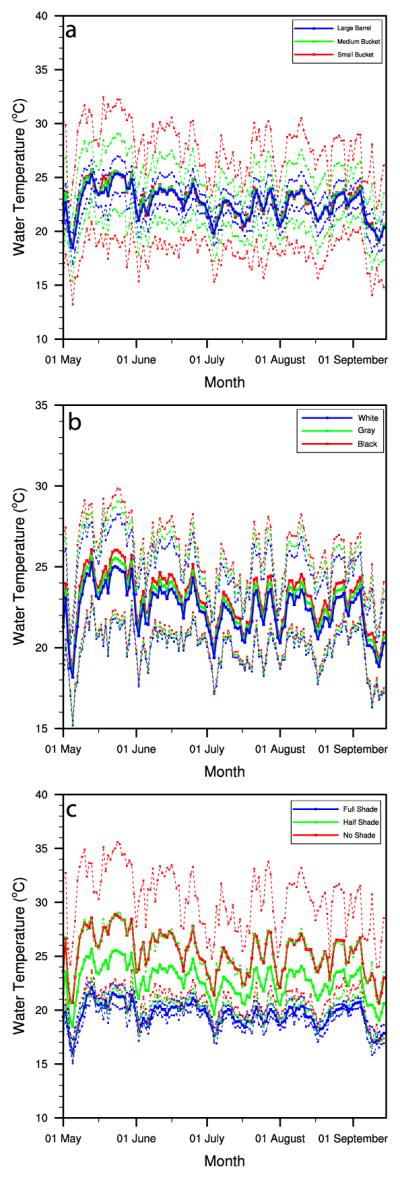
Comparison of simulated daily average water temperature (solid lines) and maximum and minimum water temperature (dotted lines), from May to September 2011 in Rio Blanco, for (a) gray containers in the form of 3.8-L bucket (red), 18.9-L bucket (green), and 208.2-L drum (blue) in half shade; (b) white (blue), gray (green), and black (red) 18.9-L buckets in half shade. (c) Gray 18.9-L bucket in full shade (blue), half shade (green), and no shade (red).

As shown in Figure 8b, the differences in reflectivity (albedo) among the various-colored containers cause substantial differences in daytime heating due to enhanced solar absorption for darker colors; these differences are not fully compensated for during nighttime since the albedo only impacts the solar (daytime) radiation balance. This means that, compared to an otherwise identical white container, a black container will 1) have a larger daily temperature range and 2) have a higher average water temperature. In our example, the water in the black container is about 1°–1.5°C warmer than the white container on average. Differences in average daily temperatures between the no shade and full shade cases are substantial: on the order of 7°C during clear-sky conditions (May and June) and less (4°C) during cloudy conditions (July) (Figure 8c). Additionally, the no shade containers have a much larger daily temperature range compared to shaded containers (12° vs 2°C) due to enhanced absorption of solar radiation.

3.2.3. Comparison of experimental results among cities

We also examined the differences among cities for several experiments (Figures 9–11). Manual filling was disabled in the presented scenarios to better understand the role of water availability in driving the differences among containers, and therefore missing values represent times when water levels were <15 mm due to the lack of rainfall. Figure 9 shows the May–September 2011 simulated daily average, maximum, and minimum water temperatures and cumulative water heights for a gray, medium-sized (18.9 L) bucket located in half shade for the three cities. Figure 10 is a summary plot showing the May–September simulated averages of water temperature and the number of days with water heights >15 mm by type of containers and city. As expected, the daily water temperature decreases with elevation from Veracruz City to Puebla City (Figure 9a). Conversely, the daily water temperature range increases with elevation (Figure 9a), which is due to less cloudy conditions (Figure 2f) and smaller volumes of water in containers due to lower rainfall (Figure 9b), in Rio Blanco and Puebla City compared to Veracruz City. The May–September average water temperatures in the containers (Figure 10a) are similar to the average air temperatures for the same period (Figure 2a); this holds true for all three container types (all gray and in half shade). Average temperatures become slightly smaller with increasing container size (3.8-L bucket vs 208.2-L drum) and larger with decreasing albedo (black vs white) and with decreasing shade or cloudiness, as demonstrated in Figure 8.

Figure 9.

Comparison of (a) simulated daily average water temperature (solid lines) and maximum and minimum water temperature (dotted lines) and (b) water height from May to September 2011 and based on a gray 18.9-L bucket in half shade for Puebla City (blue), Rio Blanco (green), and Veracruz City (red). Missing data in (a) correspond to times when water height is below the 15-mm threshold for numerical stability of water temperature estimates.

Figure 11.

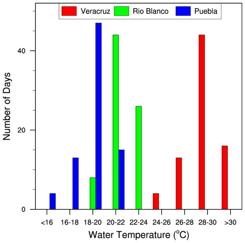
Histogram of the total number of days from May to September 2011 with simulated water height >15 mm in a gray 18.9-L bucket in half shade, by daily average water temperature, for Puebla City (blue), Rio Blanco (green), and Veracruz City (red).

Figure 10.

Comparison of (a) simulated daily average water temperature and (b) days with water height > 15 mm from May to September 2011 and based on a gray container (all three types are shown) in half shade for Veracruz City (red), Rio Blanco (green), and Puebla City (blue).

Moreover, the number of days with water heights >15 mm (Figure 10b) is noteworthy because Puebla City, which receives the least rain (Figure 2e) and therefore has the lowest cumulative water heights (Figure 9b), has the most days with water heights >15 mm. This is partly due to Puebla City receiving more rain earlier in the season (May and June) in 2011. Therefore, despite having lower temperatures, water availability does not appear to be a limiting factor for containers in Puebla City. Finally, the histogram for the number of days during May–September 2011 with simulated daily water temperatures falling within 2°C increments, based on a gray 18.9-L bucket located in half shade, illustrates the shift in typical water temperatures from low to high elevations (Figure 11). For example, water temperatures in the specified container commonly were projected to exceed 24°–26°C in Veracruz City but not in Puebla City. Conversely, water temperatures commonly were projected to be <22°C in Puebla City, whereas this did not occur in Veracruz City. These distinct water temperature differences will be important drivers of differences in immature Ae. aegypti development and survival rates (Focks et al. 1993a).

4. Conclusions

In our sensitivity simulations, WHATCH’EM was applied to project water thermodynamics in three commonly encountered container types (small buckets, medium-sized buckets, and large drums) at three representative cities located along an elevation and climate gradient that ranges from Veracruz City at sea level, where Ae. aegypti is highly abundant, to the high elevation Puebla City at ~2100 m, where Ae. aegypti is rarely found (Lozano-Fuentes et al. 2012, 2014). We found that our energy balance modeling approach adds an important level of complexity and nonlinearity to water temperature variability, leading to results that are not always intuitive. In particular, the explicit inclusion of cloud effects in WHATCH’EM plays a first-order role in container water dynamics. Accounting for clouds in such models, in addition to enhancing accuracy and model sensitivity, is also important from a climate change perspective: even if air temperatures become warmer in a given location—as they have nearly everywhere globally and are projected to continue to do so (IPCC 2013)—changes in cloudiness (for which climate projections are highly uncertain) have strong potential to amplify or dampen the corresponding changes in the magnitude and daily range of water temperature in containers at that location. Changes in the frequency and magnitude of rainfall also impact container water temperatures (by modulating the volume) and the number of days in which adequate water is available for development of mosquito immatures.

The WHATCH’EM results for water characteristics in containers in the three examined cities also provided insights into the mechanisms potentially underlying the field observation that Ae. aegypti immatures are abundant at lower elevations (<1300 m; Veracruz City and Rio Blanco) but only rarely encountered at high elevations (>2000 m; Puebla City; Lozano-Fuentes et al. 2012). Previous studies have shown that the temperature optimum for Ae. aegypti larval and pupal development, with short development times and high survival rates, is in the range of 24°–34°C (Bar-Zeev 1958; Rueda et al. 1990; Tun-Lin et al. 2000; Kamimura et al. 2002; Mohammed and Chadee 2011; Padmanabha et al. 2011b; Richardson et al. 2011; Farjana et al. 2012; Eisen et al. 2014). We found that model-projected water temperatures from May to September 2011 in a representative container (gray, medium-sized bucket located in half shade) consistently exceeded 24°C in Veracruz City and commonly exceeded 24°C in Rio Blanco but very rarely did so in Puebla City (Figure 11). Moreover, the model projected much greater daily temperature ranges of water in the containers in Puebla City compared to Veracruz City (Figure 9a), a factor that recently was demonstrated to be negatively associated with development time of Ae. aegypti larvae (Mohammed and Chadee 2011; Carrington et al. 2013b). Consequently, we speculate that suboptimal temperature conditions for Ae. aegypti immatures in containers in Puebla City presently inhibits potential for population growth of the mosquito in this high elevation city.

We also note that WHATCH’EM simulations may prove useful for examining how human–environment–container interactions impact Ae. aegypti, for example, by providing information on which containers (by size, color, and shading) have the most favorable conditions for the mosquito and thus should be specifically targeted in source reduction campaigns enacted by vector control programs or via community participation. Toward this end, future work will more comprehensively assess the impacts of water storage practices (i.e., manual filling) and container placement, shapes, and types on water characteristics. Additional validation efforts, corresponding with the sensitivity study presented here, are also desired. Finally, we also hope to explore how WHATCH’EM, or a related model building upon WHATCH’EM, could be applied to natural water bodies of limited size, which may harbor a variety of mosquitoes of medical importance including culicine virus vectors and anopheline malaria vectors.

References

- Barrera R, Amador M, Clark GG. Ecological factors influencing Aedes aegypti (Diptera: Culicidae) productivity in artificial containers in Salinas, Puerto Rico. J Med Entomol. 2006;43:484–492. doi: 10.1603/0022-2585(2006)43[484:EFIAAD]2.0.CO;2. [DOI] [PubMed] [Google Scholar]
- Bartlett-Healy K, Healy SP, Hamilton GC. A model to predict evaporation rates in habitats used by container-dwelling mosquitoes. J Med Entomol. 2011;48:712–716. doi: 10.1603/ME10168. [DOI] [PubMed] [Google Scholar]
- Bartlett-Healy K, Healy SP, et al. Larval mosquito habitat utilization and community dynamics of Aedes albopictus and Aedes japonicus (Diptera: Culicidae) J Med Entomol. 2012;49:813–824. doi: 10.1603/ME11031. [DOI] [PubMed] [Google Scholar]
- Bar-Zeev M. The effect of temperature on the growth rate and survival of the immature stages of Aedes aegypti (L.) Bull Entomol Res. 1958;49:157–163. doi: 10.1017/S0007485300053499. [DOI] [Google Scholar]
- Braks MAH, Honorio NA, Lounibos LP, Lourenco-de-Oliveira R, Juliano SA. Interspecific competition between two invasive species of container mosquitoes, Aedes aegypti and Aedes albopictus (Diptera: Culicidae), in Brazil. Ann Entomol Soc Amer. 2004;97:130–139. doi: 10.1603/0013-8746(2004)097[0130:ICBTIS]2.0.CO;2. [DOI] [Google Scholar]
- Carrington LB, Armijos MV, Lambrechts L, Scott TW. Fluctuations at a low mean temperature accelerate dengue virus transmission by Aedes aegypti. PLoS Neglected Trop Dis. 2013a;7:e2190. doi: 10.1371/journal.pntd.0002190. [DOI] [PMC free article] [PubMed] [Google Scholar]
- Carrington LB, Seifert SN, Willits NH, Lambrechts L, Scott TW. Large diurnal temperature fluctuations negatively influence Aedes aegypti (Diptera: Culicidae) life-history traits. J Med Entomol. 2013b;50:43–51. doi: 10.1603/ME11242. [DOI] [PubMed] [Google Scholar]
- Chang LH, Hsu EL, Teng HJ, Ho CM. Differential survival of Aedes aegypti and Aedes albopictus (Diptera: Culicidae) larvae exposed to low temperatures in Taiwan. J Med Entomol. 2007;44:205–210. doi: 10.1603/0022-2585(2007)44[205:DSOAAA]2.0.CO;2. [DOI] [PubMed] [Google Scholar]
- Chen F, et al. Modeling of land surface evaporation by four schemes and comparison with FIFE observations. J Geophys Res. 1996;101:7251–7268. doi: 10.1029/95JD02165. [DOI] [Google Scholar]
- Cheney EW, Kincaid D. Numerical Mathematics and Computing. Brooks/Cole; 2007. p. 763. [Google Scholar]
- Cheng S, Kalkstein LS, Focks DA, Nnaji A. New procedures to estimate water temperatures and water depths for application in climate-dengue modeling. J Med Entomol. 1998;35:646–652. doi: 10.1093/jmedent/35.5.646. [DOI] [PubMed] [Google Scholar]
- Cogley JG. The albedo of water as a function of latitude. Mon Wea Rev. 1979;107:775–781. doi: 10.1175/1520-0493(1979)107<0775:TAOWAA>2.0.CO;2. [DOI] [Google Scholar]
- Couret J, Dotson E, Benedict MQ. Temperature, larval diet, and density effects on development rate and survival of Aedes aegypti (Diptera: Culicidae) PLoS One. 2014;9:e87468. doi: 10.1371/journal.pone.0087468. [DOI] [PMC free article] [PubMed] [Google Scholar]
- Crawford TM, Duchon CE. An improved parameterization for estimating effective atmospheric emissivity for use in calculating daytime downwelling longwave radiation. J Appl Meteor. 1999;38:474–480. doi: 10.1175/1520-0450(1999)038<0474:AIPFEE>2.0.CO;2. [DOI] [Google Scholar]
- Ebert EE, Janowiak JE, Kidd C. Comparison of near-real-time precipitation estimates from satellite observations and numerical models. Bull Amer Meteor Soc. 2007;88:47–64. doi: 10.1175/BAMS-88-1-47. [DOI] [Google Scholar]
- Eisen LS, Monaghan AJ, Lozano-Fuentes S, Steinhoff DF, Hayden MH, Bieringer PE. The impact of temperature on the bionomics of the vector mosquito Aedes (Stegomyia) aegypti, with special reference to the cool geographic range margins. J Med Entomol. 2014;51:496–516. doi: 10.1603/ME13214. [DOI] [PubMed] [Google Scholar]
- Ellis AM, Garcia AJ, Focks DA, Morrison AC, Scott TW. Parameterization and sensitivity analysis of a complex simulation model for mosquito population dynamics, dengue transmission, and their control. Amer J Trop Med Hyg. 2011;85:257–264. doi: 10.4269/ajtmh.2011.10-0516. [DOI] [PMC free article] [PubMed] [Google Scholar]
- Farjana T, Tuno N, Higa Y. Effects of temperature and diet on development and interspecies competition in Aedes aegypti and Aedes albopictus. Med Vet Entomol. 2012;26:210–217. doi: 10.1111/j.1365-2915.2011.00971.x. [DOI] [PubMed] [Google Scholar]
- Focks DA, Alexander N. 2006 Multicountry study of Aedes aegypti pupal productivity survey methodology: Findings and recommendations. World Health Organization Rep TDR/ IRM/DEN/061. :56. [Available online at http://www.who.int/tdr/publications/tdr-research-publications/multicountry-study-aedes-aegypti/en/.]
- Focks DA, Haile DG, Daniels E, Mount GA. Dynamic life table model for Aedes aegypti (Diptera: Culicidae): Analysis of the literature and model development. J Med Entomol. 1993a;30:1003–1017. doi: 10.1093/jmedent/30.6.1003. [DOI] [PubMed] [Google Scholar]
- Focks DA, Haile DG, Daniels E, Mount GA. Dynamic life table model for Aedes aegypti (Diptera: Cu-licidae): Simulation results and validation. J Med Entomol. 1993b;30:1018–1028. doi: 10.1093/jmedent/30.6.1018. [DOI] [PubMed] [Google Scholar]
- Gratz NG. Emerging and resurging vector-borne diseases. Annu Rev Entomol. 1999;44:51–75. doi: 10.1146/annurev.ento.44.1.51. [DOI] [PubMed] [Google Scholar]
- Gratz NG. Critical review of the vector status of Aedes albopictus. Med Vet Entomol. 2004;18:215–227. doi: 10.1111/j.0269-283X.2004.00513.x. [DOI] [PubMed] [Google Scholar]
- Gubler DJ. The changing epidemiology of yellow fever and dengue, 1900 to 2003: Full circle? Comp Immunol Microbiol Infect Dis. 2004;27:319–330. doi: 10.1016/j.cimid.2004.03.013. [DOI] [PubMed] [Google Scholar]
- Hemme RR, Tank JL, Chadee DD, Severson DW. Environmental conditions in water storage drums and influences on Aedes aegypti in Trinidad, West Indies. Acta Trop. 2009;112:59–66. doi: 10.1016/j.actatropica.2009.06.008. [DOI] [PMC free article] [PubMed] [Google Scholar]
- Hiscox A, et al. Risk factors for the presence of Aedes aegypti and Aedes albo-pictus in domestic water-holding containers in areas impacted by the Nam Theun 2 Hydroelectric Project, Laos. Amer J Trop Med Hyg. 2013;88:1070–1078. doi: 10.4269/ajtmh.12-0623. [DOI] [PMC free article] [PubMed] [Google Scholar]
- IPCC. Climate Change 2013: The Physical Science Basis. Cambridge University Press; 2013. p. 1535. [DOI] [Google Scholar]
- Joyce RJ, Janowiak JE, Arkin PA, Xie P. CMORPH: A method that produces global precipitation estimates from passive microwave and infrared data at high spatial and temporal resolution. J Hydrometeor. 2004;5:487–503. doi: 10.1175/1525-7541(2004)005<0487:CAMTPG>2.0.CO;2. [DOI] [Google Scholar]
- Juliano SA, Lounibos LP, O’Meara GF. A field test for competitive effects of Aedes albopictus on A. aegypti in South Florida: Differences between sites of coexistence and exclusion? Oecologia. 2004;139:583–593. doi: 10.1007/s00442-004-1532-4. [DOI] [PMC free article] [PubMed] [Google Scholar]
- Kamimura K, et al. Effect of temperature on the development of Aedes aegypti and Aedes albopictus. Med Entomol Zool. 2002;53:53–58. doi: 10.7601/mez.53.53_1. [DOI] [Google Scholar]
- Kearney M, Porter WP, Williams C, Ritchie S, Hoffmann AA. Integrating biophysical models and evolutionary theory to predict climatic impacts on species ranges: The dengue mosquito Aedes aegypti in Australia. Funct Ecol. 2009;23:528–538. doi: 10.1111/j.1365-2435.2008.01538.x. [DOI] [Google Scholar]
- Koenraadt CJM, Harrington LC. Flushing effect of rain on container-inhabiting mosquitoes Aedes aegypti and Culex pipiens (Diptera: Culicidae) J Med Entomol. 2008;45:28–35. doi: 10.1603/0022-2585(2008)45[28:FEOROC]2.0.CO;2. [DOI] [PubMed] [Google Scholar]
- Koren V, Schaake J, Mitchell K, Duan QY, Chen F, Baker JM. A parameterization of snowpack and frozen ground intended for NCEP weather and climate models. J Geophys Res. 1999;104:19 569–19 585. doi: 10.1029/1999JD900232. [DOI] [Google Scholar]
- Kumar SV, et al. Land information system: An interoperable framework for high-resolution land surface modeling. Environ Modell Software. 2006;21:1402–1415. doi: 10.1016/j.envsoft.2005.07.004. [DOI] [Google Scholar]
- Lambrechts L, Paaijmans KP, Fansiri T, Carrington LB, Kramer LD, Thomas MB, Scott TW. Impact of daily temperature fluctuations on dengue virus transmission by Aedes aegypti. Proc Natl Acad Sci USA. 2011;108:7460–7465. doi: 10.1073/pnas.1101377108. [DOI] [PMC free article] [PubMed] [Google Scholar]
- Levi T, Ben-Fov E, Shahi P, Borovsky D, Zaritsky A. Growth and development of Aedes aegypti larvae at limiting food concentrations. Acta Trop. 2014;133:42–44. doi: 10.1016/j.actatropica.2014.02.001. [DOI] [PubMed] [Google Scholar]
- Lozano-Fuentes S, et al. The dengue virus mosquito vector Aedes aegypti at high elevation in México. Amer J Trop Med Hyg. 2012;87:902–909. doi: 10.4269/ajtmh.2012.12-0244. [DOI] [PMC free article] [PubMed] [Google Scholar]
- Lozano-Fuentes S, Welsh-Rodriguez C, Monaghan AJ, Steinhoff DF, Ochoa-Martinez C, Tapia Santos B, Hayden MH, Eisen L. Intra-annual changes in abundance of Aedes (Stegomyia) aegypti and Aedes (Ochlerotatus) epactius (Diptera: Culicidae) in high-elevation communities in México. J Med Entomol. 2014;51:742–751. doi: 10.1603/ME14015. [DOI] [PubMed] [Google Scholar]
- Magori K, Legros M, Puente ME, Focks DA, Scott TW, Lloyd AL, Gould F. Skeeter Buster: A stochastic, spatially explicit modeling tool for studying Aedes aegypti population replacement and population suppression strategies. PLoS Neglected Trop Dis. 2009;3:e508. doi: 10.1371/journal.pntd.0000508. [DOI] [PMC free article] [PubMed] [Google Scholar]
- Mohammed A, Chadee DD. Effects of different temperature regimens on the development of Aedes aegypti (L.) (Diptera: Culicidae) mosquitoes. Acta Trop. 2011;119:38–43. doi: 10.1016/j.actatropica.2011.04.004. [DOI] [PubMed] [Google Scholar]
- Monteith JL, Unsworth MH. Principles of Environmental Physics. Academic Press; 2008. p. 440. [Google Scholar]
- Morrison AC, et al. Temporal and geographic patterns of Aedes aegypti (Diptera: Culicidae) production in Iquitos, Peru. J Med Entomol. 2004;41:1123–1142. doi: 10.1603/0022-2585-41.6.1123. [DOI] [PubMed] [Google Scholar]
- Muturi EJ, Nyakeriga A, Blackshear M. Temperature-mediated differential expression of immune and stress-related genes in Aedes aegypti larvae. J Amer Mosq Control Assoc. 2012;28:79–83. doi: 10.2987/11-6194R.1. [DOI] [PubMed] [Google Scholar]
- Padmanabha H, Bolker B, Lord CC, Rubio C, Lounibos LP. Food availability alters the effects of larval temperature on Aedes aegypti growth. J Med Entomol. 2011a;48:974–984. doi: 10.1603/ME11020. [DOI] [PMC free article] [PubMed] [Google Scholar]
- Padmanabha H, Lord CC, Lounibos LP. Temperature induces trade-offs between development and starvation resistance in Aedes aegypti (L.) larvae. Med Vet Entomol. 2011b;25:445–453. doi: 10.1111/j.1365-2915.2011.00950.x. [DOI] [PMC free article] [PubMed] [Google Scholar]
- Padmanabha H, Correa F, Legros M, Nijhout HF, Lord CC, Lounibos LP. An eco-physiological model of the impact of temperature on Aedes aegypti life history traits. J Insect Physiol. 2012;58:1597–1608. doi: 10.1016/j.jinsphys.2012.09.015. [DOI] [PubMed] [Google Scholar]
- Prata AJ. A new long-wave formula for estimating downward clear-sky radiation at the surface. Quart J Roy Meteor Soc. 1996;122:1127–1151. doi: 10.1002/qj.49712253306. [DOI] [Google Scholar]
- Richardson K, Hoffmann AA, Johnson P, Ritchie S, Kearney MR. Thermal sensitivity of Aedes aegypti from Australia: Empirical data and prediction of effects on distribution. J Med Entomol. 2011;48:914–923. doi: 10.1603/ME10204. [DOI] [PubMed] [Google Scholar]
- Richardson K, Hoffmann AA, Johnson P, Ritchie S, Kearney MR. A replicated comparison of breeding-container suitability for the dengue vector Aedes aegypti in tropical and temperate Australia. Austral Ecol. 2013;38:219–229. doi: 10.1111/j.1442-9993.2012.02394.x. [DOI] [Google Scholar]
- Rodell M, et al. The Global Land Data Assimilation System. Bull Amer Meteor Soc. 2004;85:381–394. doi: 10.1175/BAMS-85-3-381. [DOI] [Google Scholar]
- Rueda LM, Patel KJ, Axtell RC, Stinner RE. Temperature-dependent development and survival rates of Culex quinquefasciatus and Aedes aegypti (Diptera: Culicidae) J Med Entomol. 1990;27:892–898. doi: 10.1093/jmedent/27.5.892. [DOI] [PubMed] [Google Scholar]
- Smith GC, Eliason DA, Moore CG, Ihenacho EN. Use of elevated temperatures to kill Aedes albopictus and Ae. aegypti. J Amer Mosq Control Assoc. 1988;4:557–558. [PubMed] [Google Scholar]
- Steinhoff DF, Monaghan AJ. WHATCHEM version 2.1: The water height and temperature in container habitats energy model. [accessed 15 November 2016];NCAR. 2013 doi: 10.5065/D6J67DXP. [DOI] [PMC free article] [PubMed] [Google Scholar]
- Tarakidzwa I. MS thesis. Department of Physics, University of Zimbabwe; 1997. Evaporation from class-A pans: measurements and modeling; p. 109. [Google Scholar]
- Tun-Lin W, Burkot TR, Kay BH. Effects of temperature and larval diet on development rates and survival of the dengue vector Aedes aegypti in north Queensland, Australia. Med Vet Entomol. 2000;14:31–37. doi: 10.1046/j.1365-2915.2000.00207.x. [DOI] [PubMed] [Google Scholar]
- Tun-Lin W, et al. Reducing costs and operational constraints of dengue vector control by targeting productive breeding places: A multi-country non-inferiority cluster randomized trial. Trop Med Int Health. 2009;14:1143–1153. doi: 10.1111/j.1365-3156.2009.02341.x. [DOI] [PubMed] [Google Scholar]
- Walsh RK, Facchinelli L, Ramsey JM, Bond JG, Gould F. Assessing the impact of density dependence in field populations of Aedes aegypti. J Vector Ecol. 2011;36:300–307. doi: 10.1111/j.1948-7134.2011.00170.x. [DOI] [PubMed] [Google Scholar]