Social Behaviour Shapes Hypothalamic Neural Ensemble Representations Of Conspecific Sex

Summary

All animals possess a repertoire of innate (or instinctive^1,2) behaviors, which can be performed without training. Whether such behaviors are mediated by anatomically distinct and/or genetically specified neural pathways remains a matter of debate^3-5. Here we report that hypothalamic neural ensemble representations underlying innate social behaviors are shaped by social experience. Estrogen receptor 1-expressing (Esr1⁺) neurons in the ventrolateral subdivision of the ventromedial hypothalamus (VMHvl) control mating and fighting in rodents^6-8. We used microendoscopy⁹ to image VMHvl Esr1⁺ neuronal activity in male mice engaged in these social behaviours. In sexually and socially experienced adult males, divergent and characteristic neural ensembles represented male vs. female conspecifics. But surprisingly, in inexperienced adult males, male and female intruders activated overlapping neuronal populations. Sex-specific ensembles gradually separated as the mice acquired social and sexual experience. In mice permitted to investigate but not mount or attack conspecifics, ensemble divergence did not occur. However, 30 min of sexual experience with a female was sufficient to promote both male vs. female ensemble separation and attack, measured 24 hr later. These observations uncover an unexpected social experience-dependent component to the formation of hypothalamic neural assemblies controlling innate social behaviors. More generally, they reveal plasticity and dynamic coding in an evolutionarily ancient deep subcortical structure that is traditionally viewed as a “hard-wired” system.

We performed microendoscopic calcium imaging^9,10 (Inscopix, Inc.; Fig.1a) of VMHvl Esr1⁺ neurons expressing GCaMP6s¹¹ (Fig. 1b, c; see Methods) during resident-intruder (RI) assays¹², conducted in the resident's home cage. On a given day, the implanted resident mouse engaged in five trials with (different) female intruders, shuffled with five trials with (different) male intruders (Fig. 1d). We observed no impairment in social behavior in animals habituated to the miniature microscope (Fig. 1e1, f1). Behavioural data from synchronized videos were manually scored at 30 Hz. We recorded between 175 and 300 Esr1⁺ cells per day per mouse (N=7; ∼3,400 cells imaged; see Methods).

Figure 1. VMHvl Esr1+ neurons represent intruder sex.

a, Schematic of preparation. Redrawn from Allen Mouse Brain Atlas, version 1 (2008). b, Approximate imaging plane (dashed line). c, sample frame showing active neurons. d, Experimental design. e, f, sample videoframes and ΔF/F traces. g, Raster of single cell responses (n=135 cells) ranked by response strength. h, PCC between cell responses to males and females. i, Spatial maps of averaged neuronal responses (top); sex-preferring cells (>2σ above baseline; bottom left); scatterplot of response intensities (lower right). j, Fraction of cells activated or inhibited (±2σ from baseline) by conspecifics for 10 trials (N=5 mice, 2,379 cells imaged). k, Population activity vectors in PC space estimated by PLS. l, Decoder performance following introduction of intruder (5 mice, 10 trials each). Panels e-g, i, k are from one example mouse. Center values in this and all figures are means±s.e.m.

In socially and sexually experienced residents, VMHvl Esr1⁺ neural activity was low on baseline trials but elevated by conspecifics of either sex (Fig. 1e2, f2, g; ED Fig.1a, b). Cellular response kinetics following intruder introduction varied continuously, from transient to persistent (ED Fig. 1d-f). The number of cells activated (>2σ above baseline; ED Fig.1a) by conspecifics (∼20-30%) was significantly higher than by a toy mouse (<5%; ED Fig. 1b). Repeated trials with different intruders of the same sex activated similar neural ensembles (Fig. 1g), reflected by a high Pearson's correlation coefficient (PCC) between ensemble responses to the same sex (Fig. 1h). The population activity vector during a social encounter, in principal component (PC) space (Fig. 1k, ED Fig. 2b-c), or in Partial Least Squares (PLS) regression¹³ space (ED Fig. 2a), was remarkably similar across trials with different intruders of the same sex.

Figure 2. Population activity predicts social behaviour.

a1, a2, Behavioral responses to males and females (n=5 mice; AG, anogenital). b1, b2, Example decoder accuracy. c1,c2, Decoder performance (5 mice, 10 trials each; see Methods for significance testing). d, CPs of 291 neurons, with traces from two example neurons (e) during male interactions. f, CPs for the same 291 neurons during female interactions, with two example neurons (g). h, Summary of CP values. i, Proportion of sex-preferring cells (χ² test, 3 d.o.f.). j, Response strength of tuned fractions (corrected for multiple comparisons). k, Two models of ensemble representations of behavior. In this and all figures, *, p<.05; **, p<.01; ***, p<.001, n.s., not significant (two-sided t-tests unless specified). Actual P-values for all figures provided in SI Table I.

In contrast, males vs. females activated different ensembles (Fig. 1g), and the PCC between sexes was close to zero (Fig. 1h), independent of inter-animal distance (ED Fig. 3c). Male- vs. female-preferring cells (defined as activated >2σ by one but not the other sex during social interactions) were spatially intermingled (Fig. 1i; ED Fig. 1g), consistent with prior fos-catFISH studies¹⁴. The number of male-preferring cells was ∼50% higher than the number of female-preferring cells (Fig. 1j, ED Fig. 1b)^7,14. Approximately 20% of cells activated by one sex were preferentially inhibited by the opposite sex (Fig.1j; ED Fig.1c, g, h).

Intruder sex accounted for 56%±5.2% of observed variance (ED Fig. 2a), indicating that population activity is dominated by the representation of conspecific sex. Reflecting this, a linear SVM decoder could correctly classify an intruder's sex identity with almost 100% accuracy, within 3 seconds following its introduction (Fig. 1l). Decoders trained on data from residents separated from intruders by a mesh barrier also performed accurately, suggesting that sex-specific ensembles represent sensory cues, not sex-specific behaviours (see below).

Optogenetic manipulation of VMHvl Esr1⁺ neurons evoked specific social behaviours, such as mounting or attack⁷, but behaviour-triggered average analysis of calcium transients revealed few time-locked responses during such actions^14-16. We therefore investigated whether VMHvl ensemble responses could at least predict epochs when these behaviours occurred (Fig. 2a1, a2). Linear decoders showed significantly higher than chance performance in predicting episodes of attack, sniffing or mounting (Fig. 2b, c), with errors typically affecting their precise timing. Such errors may reflect inconsistencies in the manual scoring of behaviour onset/offset, or biological factors.

Additionally, we examined whether VMH neurons might be probabilistically “tuned” to particular behaviors, by calculating the “choice probability” (CP¹⁷) for each cell, defined as the chances of correctly predicting which of two alternative behaviors is occurring, based on that neuron's activity (ED Fig. 4a). Approximately half of the cells (52-53%) were tuned for periods when social behavior occurred (Fig. 2h, dark gray). Within that category, there were cells “tuned” to sniff vs. attack males, or to sniff vs. mount females (Fig. 2d-h and ED Fig. 4).

Surprisingly, many cells' “behavioural tuning” was independent of their sex-preference (Fig. 1g): for example, “sniff male”-tuned units were equally represented among male- vs. female-preferring cells (Fig. 2i). Thus, individual Esr1⁺ neurons can participate in ensembles representing a particular sex, as well as in ensembles for specific appetitive or consummatory behaviors¹⁸ (Fig. 2k, right; ED Fig. 4c). An exception was that “attack male”- and “sniff female”-tuned cells were enriched for male- vs. female-preferring neurons, respectively (Fig. 2i). Attack-tuned cells were more strongly activated than other behaviour-tuned neurons (Fig. 2j), suggesting a higher threshold for this action^7,15.

The foregoing data were obtained from the 3^rd consecutive day of social encounter testing. Prior to day 1, mice were naïve to non-littermate conspecifics, sexually inexperienced and were individually housed following surgery for at least 4 weeks (see Methods). During initial trials on day 1, we observed little mounting or attack (Fig. 3j, day 1 and ED Fig. 5a). Surprisingly, imaging revealed many cells that responded to both males and females (Fig. 3a-c, day 1). Over the next two days, more male- or female-preferring cells were observed, while the overall percentage of active cells remained fairly constant (Fig. 3a-c, day 2, day 3). Accordingly, the PCC between the male- and female-response population vectors declined to nearly zero by day 3 (Fig. 3e, gold curve, 3f). Similar changes were observed in decoder performance or the Mahalanobis distance ratio¹⁹ between same- vs. opposite-sex trials (Fig. 3g-i). Sex-specific ensembles were stable for months in animals isolated following these trials. Interestingly, 2/7 animals imaged failed to exhibit any separation of representations, and showed neither mounting nor attack (e.g., ED Fig. 6c,d). Such “anomalous” mice were observed at similar frequencies (∼15-20%) among unoperated controls (not shown). The origin of these individual differences among inbred mice is unclear.

Figure 3. Sex-specific ensembles emerge with experience.

a-d, Ensemble representations change across three days of imaging. a, Fraction of responsive cells across pairs of consecutive trials (455 cells from 5 mice). b, Response strength (ΔF/F) for 135 cells identified across three days. c, Example spatial maps of intruder preference. d, Population vectors in PLS space. e, PCC between the trial-averaged ensemble responses on day 3 and each trial (points) for 5 mice. Significant ensemble separation commences on day 1 (post-hoc Bonferroni test corrected for multiple comparisons). f, Average PCC changes for each mouse. g, SVM decoder accuracy across days. h, Schematic description of Mahalanobis distance calculation. i, Changes in the Mahalanobis distance ratio. j, Fraction of time spent in social behaviours (N=5 mice).

To track the origins of the sex-specific cells observed on day 3, we registered 455 cells across three days of imaging (ED Fig. 7; ∼40% of all cells could be registered). Twenty-five percent of day 3 sex-preferring cells were bi-responsive on day 1, while almost half derived from cells that were initially unresponsive (<2σ above baseline) to either sex (ED Fig. 8). A minority (10%) arose from switching sex-specificity. Conversely 42% of cells active on day 1 were no longer active on day 3. These data reveal complex and dynamical changes in the response properties of VMHvl Esr1⁺ neurons during the acquisition of social experience.

The progressive separation of male vs. female representations across the 3 days of testing was accompanied by an increase in mounting and attack (Figs. 3j and ED Fig. 5a). To quantify this correlation, we computed trial-by-trial changes in the male vs. female PCC, and used non-negative LASSO²⁰ to regress the PCC for each mouse against the cumulative minutes of different social behaviours, or a weighted sum of all behaviors (Fig. 4a-c and ED Fig. 9). The strongest correlation was with mounting plus anogenital investigation (Fig. 4b), and the weakest with sniffing (Fig. 4c).

Figure 4. Social experience promotes ensemble separation.

a-c, PCC for the n^th trial vs. cumulative social experience (a), cumulative mounting and anogenital sniffing (b) or cumulative body/face-directed sniffing (c). R² values are for fit curve y = A√(x) + B (black). d, Illustration of “restricted-access” experiment. e, Ensemble separation for five mice with free access (gray) and three mice with restricted access (teal) were significantly different (one-way ANOVA). f,g, PCC decreased after two restricted-access mice received free access (day 4 and day 5; one-way ANOVA); day 3 bars duplicated from (e) to facilitate comparison. h, Cumulative time spent in behavior (n=5). i, Ensembles separate after mounting commences. j, Priming experiment. k, Males primed with females (group 2, n=4) attacked conspecific males; unprimed males (group 1, n=8) did not. l, Priming experiment adapted for imaging. m, Males primed with females fought. n, Mice primed with females (n=2) showed ensemble separation 24 hr later; Mice primed with males (n=2) did not (o).

The weak correlation with sniffing suggested that olfactory cues alone might not suffice to promote the separation of male vs. female representations. To test this, we suspended intruders by the tail (allowing sniffing, but preventing mounting or attack) throughout each 2 min trial of a standard 3-day schedule (Fig. 4d). Under these conditions the male vs. female PCC remained high at day 3 in all three mice (Fig. 4e, teal bars). However, when two of these mice (a third became ill and was euthanized) were allowed free interactions with females and males over two additional days, sex-specific representations became well separated, and mounting and attack were observed (Fig. 4f,g). Similar results were obtained using a wire mesh to block social interactions with intruders (ED Fig. 10). These data suggested that exposure to conspecific odors is insufficient to promote sex-specific ensemble separation.

Next, we investigated the temporal relationship between mounting, attack and ensemble separation. Mounting appeared before attack, in both operated (Fig. 4h) and unoperated animals (ED Fig. 5b), consistent with prior reports²¹. Ensemble separation increased significantly after the first mount, but before the first attack (Fig. 4i). These observations suggested that social experience with females might suffice to promote sex-specific ensemble separation, and attack²².

To test the latter possibility, socially inexperienced, unoperated males were “primed” in a single 30 min unrestricted interaction with females, and then tested 24 hrs later in a single, 10 min RI assay with a male (Fig. 4j). Strikingly, this priming with females (during which time mounting was observed) promoted aggressiveness in 100% of males (Fig. 4k, group 2). In contrast, control males with no priming showed no attack towards an intruder male, even after 30 min (Fig. 4k, group 1).

To determine whether sexual experience can also promote the appearance of sex-specific neural ensembles, we repeated this priming experiment while imaging Esr1⁺ neurons in naïve mice (Fig. 4l). “Probe trials” with tail-suspended intruders (3 males, 3 females, 10 sec each) were performed 10 min before, and 24 hrs after, the 30 min priming interaction with females. Strikingly, the PCC between male vs female representations was significantly reduced, in probe trials performed after (but not before) female priming, compared to the same-sex PCC (Fig. 4n). These primed mice also proceeded to attack males during the RI test on day 2 (Fig. 4m). In contrast, the male vs. female PCC was not reduced after 24 hrs in mice primed with a male on day 1 (Fig. 4o). Thus, a single 30-min priming experience with a female suffices to promote both sex-specific ensemble separation and aggression. Whether ensemble separation itself is required for attack is not yet clear.

Here we report the first imaging of neuronal activity in a deep hypothalamic structure during social behaviour in freely moving animals. Our observations in experienced mice revealed distinct and reproducible VMHvl Esr1⁺ subpopulations activated by males vs. females, suggestive of labeled lines¹⁴. Surprisingly, however, in socially isolated and sexually inexperienced animals these divergent representations were not present, but emerged with sexual experience. How can these findings be reconciled with the “innate” nature of mating and aggression^1,2? One possibility is that circuits downstream of VMH are hard-wired, but that sexual experience is necessary to direct these behaviours towards appropriate social stimuli²³. We cannot exclude that plasticity in VMHvl is “inherited” from upstream regions^24-27. Nevertheless, our findings suggest that some computational features characteristic of the hippocampus and cortex—including dynamic coding, mixed selectivity, and experience-dependent plasticity^28-30—also operate in deep subcortical circuits. More generally, our findings raise the possibility that the neural representations underlying other instinctive behaviors may also incorporate learned features.

Methods

Mice

All experimental procedures involving use of live animals or their tissues were carried out in accordance with the NIH guidelines and approved by the Institutional Animal Care and Use Committee and the Institutional Biosafety Committee at California Institute of Technology (Caltech). Esr^Cre/+ knock-in mice⁷ back-crossed into the C57BL6/N background (>N10) were bred at Caltech. The Esr1^Cre/+ knock-in line is available from the Jackson Laboratory (Stock No. 017911). Heterozygous Esr1^Cre/+ were used for all studies and were genotyped by PCR analysis of tail DNA. Mice used for data acquisition were individually housed in ventilated micro-isolator cages in a temperature controlled environment (median temperature 23 °C), under a reversed 12-h dark /light cycle. All wild-type mice used as intruders in resident-intruder (RI) assays with resident Esr1^Cre/+ mice were of the C57BL6/N strain (Charles River laboratories) purchased at 12-14 weeks of age, and group-housed at Caltech prior to use. Female mice were purchased ovariectomized and received injections of 17β-estradiol benzoate (Sigma) in sesame oil; 10 μg at 48 hours and 5 μg 24 hours preceding behavioral testing, and 50 μg of progesterone 4-6 hours prior to behavioral use³¹. All mice had ad libitum access to food and water. Mouse cages were changed weekly on a fixed day on which experiments were not performed.

Surgery

Adult heterozygous Esr1^Cre/+ males were acclimatized to the conditions of being individually housed for at least five days before undergoing surgical procedures and were operated on at 12-14 weeks of age. Prior to that time, mice were maintained with male littermates, following weaning at 3 weeks, i.e., for 9-11 weeks. Mice were anaesthetized using isoflurane (2.5% induction, 1.2-1.5% maintenance, in 95% oxygen) and placed in a stereotaxic frame (David Kopf Instruments). Body temperature was maintained using a heating pad. An incision was made to expose the skull for stereotaxic alignment using the inferior cerebral vein and the Bregma as vertical references. We based the coordinates for the craniotomy and stereotaxic injection of VMHvl on an anatomical magnetic resonance atlas of the mouse brain (AP: −4.68, ML: ± 0.78, DV: −5.80 mm), as previously described⁷. Virus injection and GRIN endoscope lens implantation were performed during a single surgery. Virus-suspension was injected using a pulled-glass capillary at a slow rate of 8-10 nl min⁻¹, 100 nl per injection site (Nanojector II, Drummond Scientific; Micro4 controller, World Precision Instruments). 15-20 minutes after the cessation of injection, the glass capillary was withdrawn and a custom built tube of hypodermic grade stainless-steel was lowered to the VMHvl target coordinates to create space that would accommodate the endoscope lens. The tube was removed after 20-30 minutes and immediately replaced by a GRIN endoscope lens (Inscopix, 0.5 or 0.6mm diameter, minimum 6mm length). The lens was cemented to the skull using a small drop of dental cement (Metabond, Parkell), and following curing thin layers of dental cement were applied to cover the entire exposed skull. Next, multiple layers of dental acrylic (Coltene, Whaledent) were applied into which a head-fixation bar was allowed to set. Once the dental acrylic cured, the mice were taken off isoflurane and allowed to recover in clean, autoclaved cages to minimize any chance of infection. Bupivacaine and Ketoprofen were administered as local and systemic analgesics respectively during surgery and mice were provided Motril and Ibuprofen in their drinking water post-surgery, for a week. Mice were maintained in isolation until recording experiments were performed (typically > 4 weeks; see below).

Virus

Esr1⁺ neurons expressing Cre recombinase in VMHvl were transduced with an adeno-associated virus (AAV) expressing GCaMP6S under the Synapsin I promoter (AAV1.Syn.GCaMP6s; Penn Vector Core). A series of titration experiments was performed to determine the highest dilution at which bright cytoplasmic, non-nuclear GCaMP6s localization could be observed in slices of fixed-tissue from injected animals³² prior to performing injections for in vivo imaging applications.

Microscope alignment

Mice were initially checked for epifluorescence signals 4 weeks after virus injection and endoscope lens implantation. Mice were anaesthetized using isoflurane, mounted in a stereotaxic frame and the head was leveled to the horizontal plane. A head-mounted miniaturized microscope (nVista, Inscopix) was then lowered over the implanted lens until GCaMP6s-expressing fluorescent neurons were in focus uniformly across the imaging plane. If fluorescent neurons were not observed, the mice were returned to housing and tested again on a weekly basis. If GCaMP6s-expressing fluorescent neurons were detected, the microscope was aligned and a permanent baseplate attached to the head according to published protocols³³. A baseplate cover (BPC-2, Inscopix) was used to prevent homecage bedding dust from settling on the lens. After 48 hours, the baseplate cover was replaced by a weight-matched dummy microscope (DMS-2, Inscopix), to acclimatize the mouse to the weight of the microscope for at least three days before social behavioral testing.

Selection of animals for imaging experiments

Imaging data were collected from a total of 25 Esr1^Cre/+ mice (out of 122 injected/implanted animals generated in multiple cohorts). Of these 25 implanted animals, 16 were used for experiments reported in this paper. Mice were selected for combined imaging and behavior experiments based on the following criteria: 1) they yielded individually discernable neurons across at least half the imaging field; 2) the imaging plane was clear and not occluded by blood or debris; and 3) image registration could be applied successfully to correct for motion artifacts (all but one mouse). The most frequent failure modes were mis-targeting of VMHvl by the viral injection and/or GRIN lens implantation; inadequate levels of GCaMP6s expression; and failure to obtain a clear imaging plane.

Determination of sample size

For imaging experiments, between 3 and 7 mice were imaged per experimental paradigm; the number of mice was dependent on the yield of usable mice and the number of animals initially implanted and injected. Selection of mice was determined by screening with the miniscope before experimentation (see above 2 sections). Selection was not based on any pre-specified effect. Data presented in Figs. 1-3 is from 5/7 mice imaged that eventually showed mounting and attack behaviour by the third day of imaging. The two ‘anomalous’ mice that showed neither consummatory social behaviour (mating, fighting), nor a separation of ensemble representations, were treated separately; one such (mouse 6) is illustrated in ED Fig. 6.

The sample size for the number of cells was 175-300 cells per mouse, and was affected by the volume of viral GCaMP6s injected, the efficiency of Cre-mediated recombination and level of expression. While post-processing the imaging data (after PCA-ICA identification of individual cells) 1-5% of the identified components were discarded as artifacts and rest 95-99% were treated as cells and used for further analysis.

Sample sizes for behavioral experiments were determined by the current standard used for mice in behavioral neuroscience experiments, based on the minimal amount of mice required to detect significance with an alpha rate set at .05 in a standardly powered experiment.

Randomization

Animals were assigned randomly to experimental and control groups.

Blinding

The investigators were not blinded during imaging data collection. Blinding was used during analysis where the social behaviors were scored blind to the sex of the intruder mouse. Computational analysis was not performed blinded.

Resident-Intruder assay

Before resident-intruder testing implanted mice were individually housed for at least 4 weeks, to allow recovery from surgery and adequate levels of GCaMP6s expression. The resident-intruder assay was adapted for social interactions while imaging neuronal activity. The lens-implanted Esr1^Cre/+ mouse was always the homecage resident. Data were collected from each resident over three consecutive days of testing, beginning when the resident was still naïve to adult non-littermate conspecifics (i.e., housed in social isolation beginning 5 days prior to surgery). The results in Figs. 1 and 2 are derived from resident animals on their third day of testing, by which time most of them expressed normal sexual and aggressive behaviors. Data on each day were collected as a sequence of 14 individual trials, comprising 2 baseline trials (i.e. trials performed in the absence of an intruder/object), 2 trials with a toy mouse (OurPets Play-N-Squeak) and 5 trials each with a male or female intruder. The sequence of trials with an intruder or object was interleaved; the sex of the first intruder was randomized across animals. Each trial with an object or intruder lasted 2-3 minutes, to minimize photobleaching of GCaMP6s, and was preceded and followed by 30 s of imaging before and after the intruder was introduced, respectively. Intruders were manually introduced into the resident's homecage held by the tail, during which the residents were allowed to anogenitally investigate the intruders. Care was taken to remove the intruder or toy from the arena only when the resident was at a distance to prevent artificially truncating any naturally occurring social interaction. The inter-trial interval was 10 minutes. A different intruder mouse was used for each trial with a male or female intruder. One cohort of 7 implanted mice were used for imaging in these 3-day assays; of these 7 mice, 2 did not show mating or aggressive behaviour or ensemble separation and were omitted from the analyses performed in Figs. 1-3 (see main text). Another cohort of 12 unoperated mice was used for behavioral analysis only (Fig. 4j-k). A third cohort of 3 implanted mice was used for the restricted-access assay (Fig. 4d-g); a fourth cohort of 6 implanted mice was used for imaging in the female “priming” assay in Fig. 4l-o.

Restricted-access assay: held-intruder

For a first group of implanted mice (n=3), experimental design was identical to the resident-intruder assay, however to prevent free social interaction, intruder mice were held by the experimenter for the duration of each trial. Interactions with five males, five females, two toy and two baseline trials were recorded for each resident each day, for three consecutive days of testing. The same implanted mice were subsequently given two additional consecutive days of testing in the original resident-intruder assay (see previous section). One of the 3 implanted mice became ill and had to be euthanized following the restricted-access portion of the experiment.

Restricted-access assay: mesh barrier

For a second group of implanted mice (n=2), experimental design was identical to the resident-intruder assay, however intruders were placed inside a wire-mesh barrier (an inverted pencil cup) when introduced into the resident's home cage. Interactions with five males, five females, two toy and two baseline trials were recorded for each resident each day, for three consecutive days of testing. The mice were subsequently tested for two consecutive days of social interactions as in the primary resident-intruder assay (days 4, 5), followed by an additional day of testing with intruders behind the mesh barrier (day 6).

Priming assay (Fig. 4l-o)

Naive implanted mice were allowed to freely interact in a single session with either a female or a male for 30 minutes on day 1 (“priming”), and then tested with a conspecific of the opposite sex on day 2 in a 10 min free interaction trial. Before and after the priming on day 1, “probe” trials were performed with (different) probe animals of each sex (n=3 males, n=3 females), to test for ensemble separation before vs. after priming. During these probe trials, a male or female probe animal was suspended by the tail in the cage for 10 seconds, during which time sniffing (but no attack or mounting) by the implanted resident occurred. Three implanted mice were primed with females on day 1, and three mice primed with males on day 1. Of the 3 mice primed with females, one mouse failed to mate with the female during priming, or to show aggression towards a male on day 2, and was omitted from imaging analysis, since the purpose of the experiment was to ask whether ensemble separation correlated with the appearance of aggression following the priming interaction with females. (This mouse may have been one of the ‘anomalous’ mice we describe, which exhibited neither mating or fighting.) Of the 3 mice primed with males on day 1, one that already showed a sex-specific ensemble separation on the first probe trial (day 1) i.e., prior to priming, was omitted from the analysis, as the purpose of the experiment was to ask whether priming with a male was sufficient to cause sex-specific ensemble separation.

An additional 12 unoperated mice that had been socially isolated for 2 weeks were tested in this priming assay only to quantify behavior. 4 mice were presented with a female on day 1, and 8 mice only experienced a single, 30 minute encounter with a male on day 2.

Neuronal and behavioral data acquisition

Mice were temporarily head-fixed prior to imaging sessions and the head-mounted dummy was replaced by the miniaturized microscope. Anaesthesia was not used at this step because it strongly suppressed hypothalamic neuronal activity. The mice were placed in their home cages situated within the behavioral arena with head-mounted microscopes attached, and allowed to habituate 15-30 minutes prior to data acquisition. The behavioral arena was custom built (all parts from Thorlabs) with one top-view and one side-view camera (Flea3, Point Grey), for acquiring behavioral data, saved as AVI files on a Windows computer. A TTL pulse from the Sync port of the Data Acquisition Box (DAQ, Inscopix) of the microscope was used to trigger individual frames through the GPIO pins on the camera. This allowed a 1:1 correspondence between behavioral frames and neuronal imaging frames, necessary for synchronizing neuronal activity to behavior. Shortly before data acquisition the imaging parameters were configured and saved using nVista (Inscopix) control software. All but two mice used in this study were imaged at 30 Hz with 33.2 ms exposure per frame (the other two were imaged at 15 Hz with 66.2 ms exposure per frame, as they exhibited lower levels of GCaMP6s fluorescence). Microscope LED illumination was 11-14% of the maximum allowed, at 2-2.75× gain. The field of view was cropped to the region encompassing the fluorescent neurons to maximize uninterrupted data acquisition at 30 Hz. All imaging parameters were saved and were the same for every trial for each mouse. Data were saved as stacks of frames in TIFF or RAW format.

Position tracking

Instantaneous positions and poses (estimated by a fit ellipse) of both mice was tracked from top-view video, using custom software written in MATLAB³⁴. The distance between animals was defined as the distance between the centroids of the fit ellipses.

Data processing

The behavioral videos were loaded into Matlab using a custom-scripted behavioral annotator ^7,14 and a trained individual blind to the experimental design annotated the videos frame-by-frame for attack, mounting, head and/or flank-directed sniffing (“sniffing”) and anogenital sniffing (“AG sniffing”).

Imaging frames were spatially downsampled by a factor of two (i.e., 0.5×) in the X and Y dimensions, and normalized by dividing by a spatially band-passed version of the frame (lower bound 100 μm, upper bound 10,000 μm). Frames collected over the course of a single day were concatenated into a single stack and registered to each other to correct for motion artifacts using the Mosaic software package (Inscopix)^18,33. Imaging data were calculated as relative changes in fluorescence, ΔF(t)/F₀=(F(t)- F₀)/F₀, where F₀ was the mean of all frames across the stack. To extract single cells and their Ca²⁺ activity traces from the fluorescent imaging frames, we applied an established computational algorithm for cell sorting based on Principal Component and Independent Component Analyses (PCA/ICA)³⁵ to generate a series of spatial filters that each corresponded to a single cell. Filters were individually, manually inspected, and those unlikely to correspond to single neurons were discarded^10,33. Thresholded, segmentation masks for each spatial filter (i.e., cell) were projected onto the ΔF(t)/F₀ stack of frames to extract time-course of fluorescence changes for that cell. On average we identified 228±64 cells per mouse per day using PCA/ICA (total of 3,396 cells imaged in 7 mice; 2,379 cells from the 5 mice that showed mounting and attack). For each cell, ΔF(t)/F₀ traces were normalized by the standard deviation of the first baseline trial, and reported in units of standard deviation (σ).

Registration across days

Individual spatial filters, each corresponding to a cell, for each day of imaging, were thresholded and combined into maximum intensity projection maps (ED Fig.7). Intensity-based image registration was used to identify a pair of affine transformations for aligning the day 1 and day 3 maps to the day 2 map. Overlapping filter triplets from the three days were manually screened for accuracy. All selected triplets had an average of less than 3 microns Euclidean distance between centroids on pairs of days (day 1 vs day 2, day 2 vs day 3, and day 1 vs day 3; average centroid separation of registered filters = 0.98 ±0.03 microns). Roughly 40% of all spatial filters (cells) were registered across three days of imaging (n = 99±37 cells per mouse).

Ensemble response vector

The time-averaged ΔF(t)/F₀ activity of each cell was computed over all frames of social interactions (sniffing, mounting or attack) during each trial, and concatenated into a N × 1 vector (N=cells) called the ensemble response vector. The use of responses from periods of social interaction precluded any effects of inter-animal distance¹⁵ in our representations. Note that the same analyses using different epochs during a trial (e.g. only frames from periods of sniffing, or distance-based criteria) did not fundamentally change our observations (ED. Fig. 3).

Quantifying distance modulation of cell responses

Cells excited or inhibited by conspecifics (mean |ΔF(t)/F₀|>2σ during periods of male- or female-interaction) showed varying degrees of modulation by the distance to the intruder. To quantify distance modulation of responsive cells, we used the distance (d) between centroids of the two mice (see Position Tracking) to identify frames in which the two animals were not interacting (and were not within ±1 sec of interaction) and were close (d < 35% diagonal length of cage; ED. Fig. 3) or far (d > 70%). r_close and r_far were measured as the average ΔF(t)/F₀ of each cell under each distance condition and used to compute a distance modulation index (m) as m |r_close – r_far|/(|r_close| + |r_far|); a measure of the extent to which cell activity varied with inter-animal distance.

Pearson's Correlation Coefficient of male-female similarity

Since on any given trial the imaged resident encountered a conspecific of one sex, the Pearson's correlation coefficient (PCC) was computed between a given trial's ensemble response vector and the average ensemble response during the two nearest neighboring trials of the other intruder sex. For the first and last trials only the one temporally closest other-sex trial was used.

Fraction of variance captured by intruder sex

The Difference of Covariances (DoC) method³⁶ was used to identify the two largest male- and female-specific sources of variance in the ensemble response, as follows. For a resident mouse on a given day, the covariance matrix between cells on all male trials (C_M), and on all female trials (C_F) was generated, and their difference C = C_M – C_F found. By construction, the eigenvectors of C with the largest positive and negative eigenvalues correspond to the largest male- and female-specific sources of variance, respectively. To measure fraction of variance captured by this pair of eigenvectors, the N × T (neurons by time) matrix of ensemble activity on a given day of imaging was reconstructed as a weighted sum of these two vectors using linear regression. The R² value of the reconstruction was reported as the fraction of variance captured.

Dimensionality reduction

Low-dimensional representations for visualizing changing ensemble dynamics in time were constructed using PCA³⁷ or PLS regression³⁸ (using the plsregress function in MATLAB). For PLS, all traces from a day of imaging were concatenated and regressed against a 1 × T vector with entries valued at -1 (if a male intruder was present), 1 (if female intruder) or 0 (otherwise).

Decoding intruder sex (Fig. 3f)

To determine whether VMHvl activity contained information about intruder sex, a linear decoder was used to decode the sex of the intruder from ensemble activity during periods of social interaction. Training data was constructed from the set of N×1 (N=neurons) ensemble activity vectors from all frames occurring during social interaction. To avoid effects of data set size across imaged mice, a random subset of 50 cells was drawn from the set of all cells imaged that day. This training data, along with intruder sex labels, was then used to train a linear Support Vector Machine (SVM) decoder³⁹. Decoder performance was evaluated using cross-validation, by excluding all data from one intruder during training and using that data to test decoder performance; this was repeated 15 times for each intruder, each time with a different random subset of cells, and performance computed as the average accuracy across test sets. Analysis was repeated for each day of imaging, with a separate decoder trained for each day.

Decoding intruder sex following intruder introduction (Fig. 1l)

We wanted to identify how quickly, from the moment the intruder entered, a linear decoder could predict the sex of the intruder from the ensemble activity. The decoder performance was tested in half-second windows, starting 5 seconds before to 10 seconds after, the moment, the intruder fully entered the resident's homecage. The training set was constructed by averaging the ΔF(t)/F₀ for each cell within a 0.5 second time bin centered at a time t, for each male and female trial on one day (typically 10 trials total). Overfitting to the small (n=9) number of training examples was reduced by projecting training data onto the first 10 PCs of ensemble activity from that day; we found that this improved decoder performance. The projected data and intruder sex labels were then used to train a linear SVM decoder, and decoder performance was evaluated using leave-one-out cross-validation with each trial held out once. To allow for dynamic changes in intruder-evoked responses, a new decoder was trained at each time point.

Decoding behavior (Fig. 2b)

To determine whether ensemble activity contained information about specific social behaviors, a separate binary linear decoder was trained for each behavior, to predict whether the behavior was occurring or not. To avoid confounding representations of behavior with representations of intruder sex, separate decoders were trained for male- and female-directed behaviors. Training data was constructed from the set of N×1 ensemble activity vectors from all frames of all day 3 trials with a given intruder sex, labelled positive/negative for a target behavior. Negative training data (i.e., data from periods when the behaviour of interest was not occurring) was under-sampled to produce an equal number of positive and negative training examples. These binary labels and their corresponding ensemble activity vectors were then used to train a linear SVM decoder. Decoder performance was tested via cross-validation by excluding all data from one intruder during training, and computing the average decoder performance on the held-out data using the F1 score (see below). Testing was repeated for each intruder, and for 15 instantiations of each training set.

Measuring performance of behavior decoders (Fig. 2c)

Because most behaviors occured on a small fraction of tested frames, reporting the Accuracy (true positives + true negatives)/(total samples) of a trained behavior decoder could be misleading. Instead, we reported the F1 score^40,41, computed from the decoder's Precision (= [true positives / (true positives + false positives)], i.e., the fraction of total predicted positives that are actual (ground-truthed) positives; and Recall (= [true positives / (true positives + false negatives)], i.e., the fraction of actual (total ground-truthed positives) that are correctly predicted as true positives) as F1 = 2(precision * recall)/(precision + recall).

To determine significance of the F1 score, chance F1 scores of trained SVMs were computed by shuffling both the cells and the behavior annotations. To permute behavior annotations while preserving their temporal structure, all behavior bouts and all inter-bout intervals were identified for a given day/intruder sex/behavior, and synthetic behavior rasters were constructed by randomly drawing without replacement from the set of bouts and the set of inter-bout intervals. The trained SVM weights were applied to the shuffled cells, and computed the F1 score relative to the shuffled behavior. Each form of shuffling was repeated 100×, giving 10,000 shuffled observations; we considered observed F1 scores as significant if they fell above the 97.5 percentile of the distribution of chance F1 scores.

Mahalanobis distance (Fig. 3h, i)

For each imaged mouse, the Mahalanobis distance was used as an additional measure of male and female representation separation. Two distributions of N-dimensional (N = neurons) ensemble response vectors from all imaging frames during which social interaction occurred were generated: one distribution from male trials and the other from female trials. The Mahalanobis distance (d) between each vector (the “test vector”) and these two distributions were computed, to give d_same (distance to points of the same sex as the test vector) and d_opp (distance to points of the opposite sex), which were then averaged across all test vectors. Points within the distributions that came from the same trial as the test vector were omitted during distance calculation.

Choice probability (Fig. 2d-h)

The “choice probability” (CP) was employed as a measure of a cell's tuning: how well two conditions could be predictively discriminated from a single cell's activity¹⁷. The CP of a given cell, for a pair of (behavioral) conditions, was computed by constructing a histogram of that cell's ΔF(t)/F₀ values under each of the two conditions. These two histograms were plotted against each other to generate an ROC (receiver operating characteristic) curve. The integral of the area under this ROC curve generated the CP value for each cell, with respect to each of the two behavioral conditions (see ED Fig. 4). This CP value is bounded from 0 to 1, where a CP of 0.5 corresponded to no difference between conditions. To compare two behaviors (such as sniff and attack) using this method, all frames from all behavior bouts lasting two or more seconds were used to construct the ROC curve, combining data from the second and third day of imaging. Cells from mice that spent less than 2% of time engaging in any of the four examined behaviors (attack, mounting, male-directed sniffing, and female-directed sniffing) were omitted from this analysis, due to noisiness of their CP estimates.

The significance of a cell's CP, relative to chance, was computed using shuffled bout timings for the two compared conditions (as was done for estimating chance decoder performance). Shuffling was repeated 100×, from which the mean and SD of shuffled CPs was estimated. Any observed CPs ≥ 2SD above the shuffled mean was considered significant.

Nonnegative LASSO regression of behavior against ensemble separation (Fig. 4a-c)

To identify behavioral correlates of ensemble separation, the PCC and the cumulative time spent engaging in each behavior was computed for each animal and trial (∼30 trials/mouse; N=6 mice for which imaging data was available for all three days; this includes 1 of the 2 mice that did not show mounting or attack, and whose sex representations did not segregate). The weighted sum of cumulative behaviors most correlated with the PCC was found using a nonnegative least-angle regression (LARS) implementation of LASSO²⁰, to impose sparseness and nonnegativity constraints on the fit weights. The sparseness parameter of LARS was selected to minimize the cross-validated mean squared error of the fit. For all behaviors, a square-root transform of cumulative behavior times, prior to LASSO regression, increased their correlation with the PCC.

Code and data availability

Custom code written for the purpose of this study is accessible at https://github.com/DJALab/VMHvl_imaging. Imaging and behavioral data will be made available upon reasonable request.

Extended Data

Extended Data 1. Properties of Esr1+ neuron responses.

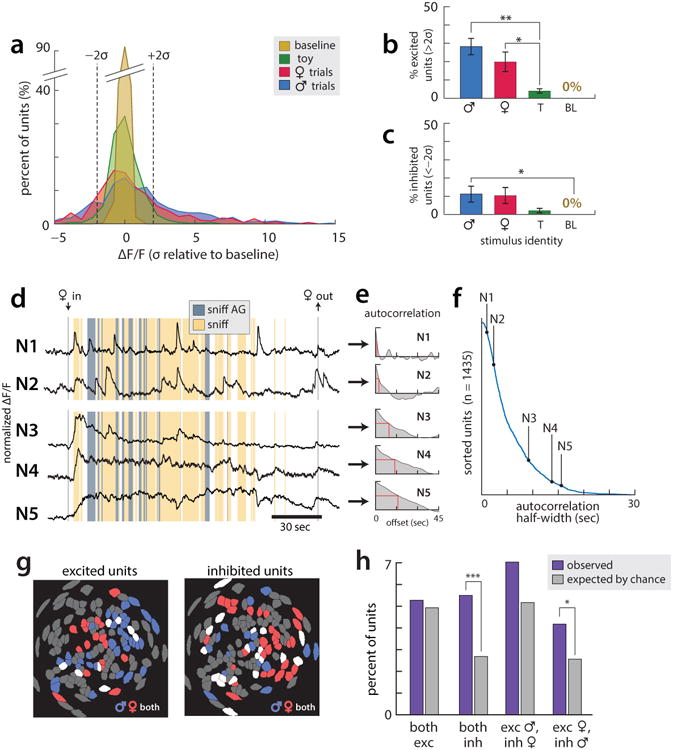
All data presented is from the third day of imaging. (a) Histogram of time-averaged ΔF(t)/F₀ values observed in the 30 seconds following stimulus introduction (or the first 30 seconds of imaging, on baseline trials). Dashed lines indicate thresholds for identifying excited ≥2 standard deviations (σ) of baseline above the mean pre-intruder baseline) and inhibited (≤−2σ below pre-intruder baseline) cells. (N=5 imaged mice, 5 male trials/5 female trials/2 toy trials/2 baseline trials per mouse.) (b-c) Average percent of time cells spend excited (b) or inhibited (c) in first 30 seconds of imaging. (d) Example traces from single Esr1+ cells, showing example response profiles across a single trial of interactions with a female conspecific. While some cells showed transient calcium responses (N1-N2), others showed slower dynamics (N3-N5), including persistent elevation or suppression of activity for the duration of the encounter with the female. We believe the latter responses to reflect the ongoing activity of some VMHvl cells, as filtered by the slow dynamics of GCaMP6s. (e) Autocorrelation functions computed across all day 3 trials, for each example cell in (d); red line indicates half-width. (f) Autocorrelation half-width computed across all day 3 trials, for all cells from the third day of imaging in all mice (N=1435 cells in 5 mice), sorted from smallest to largest, revealing a continuous range of values. Autocorrelations of the five cells in (d) are indicated. (g) Example spatial maps of excited (Left; mean ΔF(t)/F₀ ≥2σ during periods of social interaction) and inhibited (Right; mean ΔF(t)/F0 ≤−2σ during interaction across all male and female trials on the third day of imaging) cells in the presence of male and female conspecifics.

(h) The percentage of cells across all mice (N=5) that were excited and/or inhibited by both males and females, compared to the percentage expected by chance assuming statistical independence. (both inh, p=2.17e-4; exc female + inh male, p=0.0299)

Extended Data 2. Representations of males and females in PC-space in all mice.

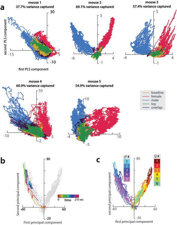
(a) Day 3 ensemble representations of intruder sex for the five mice that mounted and fought with conspecifics, projected onto the first two PLS axes. Traces are colored by intruder sex identity. Percent variance explained by the first two PLS components is noted for each mouse. (b) Projection of a single trial onto first 2 principal axes of one example mouse (mouse 2), color-coded to highlight temporal trajectory of the ensemble representation during the trial. Principal axes were identified using PCA (same axes as in Figure 1K.) (c) All trials from mouse 2, colored by trial number.

Extended Data 3. Distance dependence of intruder sex representations.

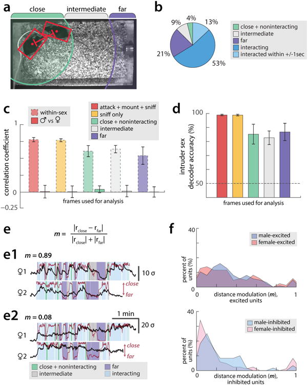
(a) Example video frame showing estimates of resident and intruder poses and centroids (red bounding boxes and points, respectively), produced by an automated tracker (Dollar et al.). Green, gray, and purple bars mark the inter-mouse distances (relative to the resident) categorized as close, intermediate, and far. (b) Proportion of time animals spent either interacting with conspecifics or present within the three zones. Timepoints in which animals have recently interacted (ie interaction occurs within ±1 s) are shown as their own category as a control for the effect of GCaMP smoothing on transient representations. (c) Pearson's correlation coefficient within trials of the same intruder sex, or between male and female trials, where representations of intruders are computed by averaging each cell's ΔF(t)/F₀ across the indicated subsets of imaging timepoints. (d) Accuracy of a linear SVM decoder for intruder sex, using representations computed as in (c). (e) The distance modulation index (m), a measure of the extent to which cell activity is modulated by inter-animal distance, is computed from r_close –the average response of a cell when animals are close but have not recently interacted (within ±1 sec), and r_far –the average response of that cell when animals are far apart and have not recently interacted. (e1-e2) Example traces from two cells that have a high (e1, m = 0.89) and low (e2, m = 0.08) distance modulation index. (f) Histograms of values of m observed in all cells that are significantly excited (Above) or inhibited (Below) during interaction with males or females. Note that inhibited cells are less sensitive to inter-animal distance than are excited cells, and that the distribution of m is similar for male- and female- responsive cells.

Extended Data 4. Choice probability histograms and example cells.

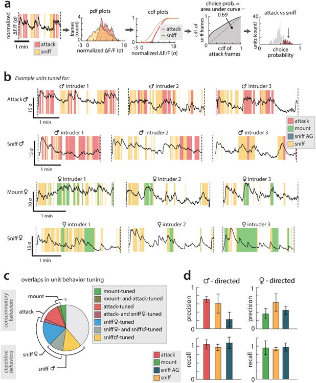
(a) Steps for computing choice probability (CP), a measure of the discriminability of two conditions, given the ΔF(t)/F₀ of a single cell. For a given pair of behaviours (here, male-directed attack and sniffing), we find the distribution of ΔF(t)/F₀ values for this cell for each behaviour and compute the cumulative distribution function (cdf). The area under the receiver operating characteristic (ROC) curve formed from these two distributions is defined as the cell's choice probability. (b) ΔF/F traces and corresponding behavior rasters from example cells that showed significant CPs for the specified behavior, illustrating the relative changes in ΔF/F and behavior. Three representative trials are shown (same examples as in Figure 2 d-g). (c) Proportion of cells significantly tuned for each examined behavior. Overlap between blocks reflects the proportion of cells that were significantly tuned for both behaviors. Note that cells cannot be tuned for both attack and male-directed sniffing, nor for both mounting and female-directed sniffing, as cells' CP is defined by comparing ΔF(t)/F₀ values under these paired conditions. All cells significantly tuned for attack, mount or sniff also showed a significant CP for periods of close social interactions (CSI, including sniffing and/or mount or attack) vs. periods of non-social interactions, by construction. However some cells that showed a significant CP for CSI vs. non-social periods did not show a significant CP for a specific behavior (see Fig. 2h). (d) Separate precision (true positives / (true positives + false positives)) and recall (true positives / (true positives + false negatives)) scores for the behavior decoders presented in Fig. 2b-c. The F1-score (presented in Fig. 2c) is defined as 2*(precision * recall) / (precision + recall).

Extended Data 5. Expression of social behaviors across trials and days.

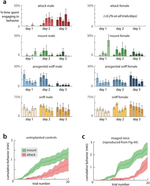
(a) Percent of time mice spent engaging in male- and female-directed behaviors on each of five trials on three days of imaging. (n=5 mice, mean ±s.e.m.) (b) Cumulative time spend mounting and attacking by a set of unoperated, socially isolated mice that underwent two days of the standard social experience paradigm depicted in Fig. 1d (n=8 mice). The unoperated mice exhibit a delay in the appearance of mounting, and show mounting before attack, indicating that changes in behavior are not due to effects of surgery or the presence of the scope. (c) Comparable data for implanted mice (n=5), reproduced from Figure 3g and restricted to the first 20 trials for comparison.

Extended Data 6. Comparison of the social behaviors and neural representations in example mice that did and did not show aggression.

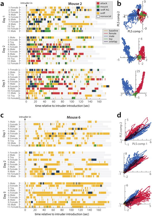
(a, c) Behavior rasters and (b, d) first two PLS components from example mice that did (a, b) and did not (c, d) show aggression to conspecific males by the third day of imaging.

Extended Data 7. Registration of cells across three days of imaging.

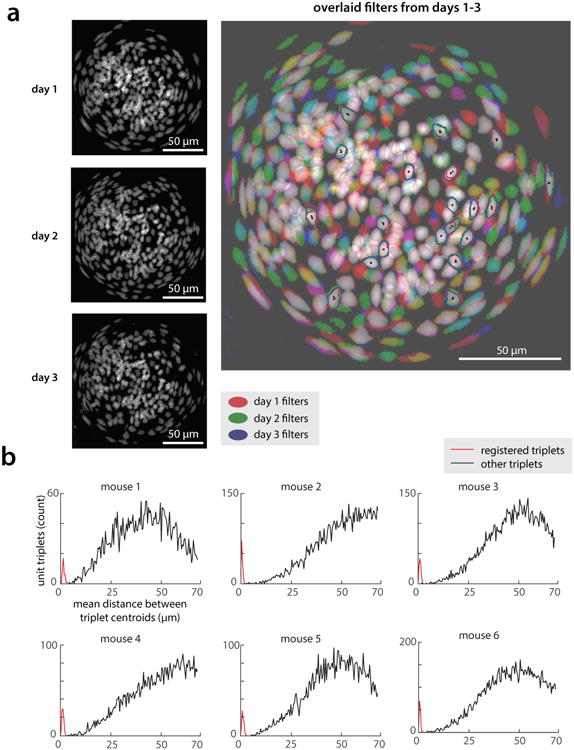
(a) (Left) Maximum projection maps of all spatial filters from each of three days of imaging in an example mouse. (Right) RGB composite image of the three left images (day 1 = red channel, day 2 = green channel, day 3 = blue channel), showing overlap of registered filters (overlap in all three channels appears in white). Outlined are 20 example cells (out of 135) that could be identified in all three days of imaging: red/green/blue lines indicate filter outlines on first/second/third day, respectively; black points mark filter centroids. (b) Histograms of average distance between filter centroids from days 1-3, in cells that could be tracked across days (red) as compared to random triplets of cells (black). Day 1-3 centroids from tracked cells were separated by an average of 2.15±0.06 microns (mean ± s.e.m., n = 593 cells tracked across days in 6 mice, during standard RI assay).

Extended Data 8. Preference changes of Esr1+ neurons during the acquisition of social experience.

(a) Table comparing responses on day 1 trial 1 to active cells on day 3, for all mice and all cells that were registered across three days of imaging (n=455 cells analyzed in the 5 mice that showed attack/mounting by day 3 of the standard RI assay). (b) Upper, response properties of cells on day 3, conditioned on their responses on day 1 trial 1, grouped according to the response types on trial 1. For example, among cells that responded to both males and females on day 1 trial 1, ∼26% (20/78) specifically responded to males on day 3, ∼26% responded specifically to females; additionally, ∼35% responded to neither sex and ∼13% responded to both. The percentages of these categories are summarized in panels (c). (b) Lower, response properties of cells on day 1 trial 1 conditioned on their response properties on day 3, grouped according to response types on day 3. The percentages in different categories are summarized in panel (d). For example, of the cells that showed male-specific responses on day 3, ∼54% derived from cells that responded to neither sex on day 1 trial 1; 20% derived from cells that responded to both sexes, 10% derived from initially female-specific cells and 16% derived from initially male specific cells. Numbers used to calculate the percentages are from the table in (a). (e) Analysis of the day 1 preferences of cells that responded only to males or only to females on day 3.

Extended Data 9. Behavior correlation with male/female similarity.

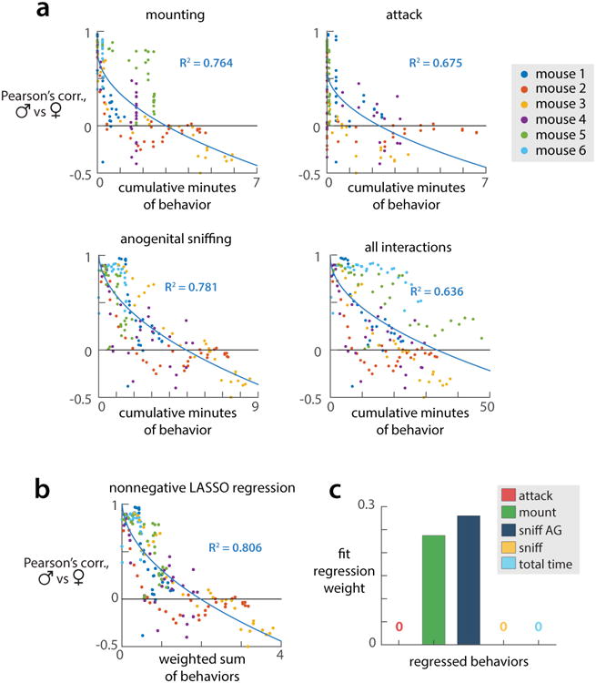
(a) Cumulative minutes of each behavior by the n^th trial plotted against the PCC between male and female representations on that trial, for 5 mice (behaviors already presented in Fig 4A-C have been omitted). All trials from a given mouse are shown in the same color. Solid lines are square root fits (of the form Y = m sqrt(X) + b) of the plotted points from all mice. (b) A weighted sum of cumulative minutes of each recorded behavior (attack, mounting, anogenital sniffing, and other sniffing) as well as cumulative time spent interacting with conspecifics, plotted against PCC between male and female representations; weights fit via nonnegative LASSO regression. (c) Bar plot of weights used to generate plot in (b), fit via nonnegative LASSO with sparseness parameter chosen to minimize mean-squared error on held-out data (see Methods).

Extended Data 10. Restricted access using a mesh container.

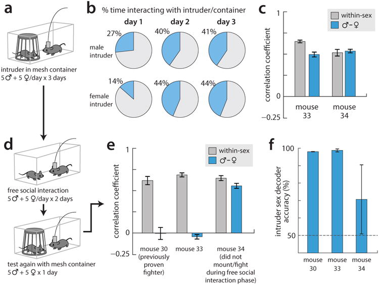
To avoid the possibility that the lack of representation separation found in Fig. 4m-p was due to the presence of the experimenter's hand during access-restricted trials, we repeated this experiment with the intruder mouse instead kept within a wire mesh container. (a) Diagram of experimental setup. (b) Percent time the imaged mouse spent interacting with the intruder on each of the three days of exposure (n=2 mice). Aside from day 1, the presence of the container does not reduce the time the resident spent investigating the intruder mouse. (c) Pearson's correlation coefficient (PCC) between male and female representations on the third day of the assay (blue bars) shows that little separation of representations has occurred in the two imaged mice. Gray bars show the average PCC between pairs of male trials or pairs of female trials, for comparison. (d) Following the three days of intruder + container presentations, mice were given two days of free social interaction, before a final day (day 6) in which intruders were again presented within the mesh container. A third, experienced animal (mouse 30) was also tested with the mesh container. (e) PCC between representations of males and females presented within the mesh container on day 6; gray bars again show average PCC between pairs of male trials or pairs of female trials. Two out of three tested mice showed clear separation of male and female representations; the third did not, but this mouse also failed to fight or mate with conspecifics during the free social interaction. (f) Performance of an SVM decoder trained to predict intruder sex from the data on day 6, showing high accuracy in the two mice that had previously fought and mounted.

References

- 1.Tinbergen N. The study of instinct. Clarendon Press; 1951. [Google Scholar]
- 2.Lorenz K. On Aggression. Harcourt, Brace & World; 1966. [Google Scholar]
- 3.Root CM, Denny CA, Hen R, Axel R. The participation of cortical amygdala in innate, odour-driven behaviour. Nature. 2014;515:269–273. doi: 10.1038/nature13897. [DOI] [PMC free article] [PubMed] [Google Scholar]
- 4.Newman SW. The medial extended amygdala in male reproductive behavior. A node in the mammalian social behavior network. Annals of the New York Academy of Sciences. 1999;877:242–257. doi: 10.1111/j.1749-6632.1999.tb09271.x. [DOI] [PubMed] [Google Scholar]
- 5.Veening JG, et al. Do similar neural systems subserve aggressive and sexual behaviour in male rats? Insights from c-Fos and pharmacological studies. European journal of pharmacology. 2005;526:226–239. doi: 10.1016/j.ejphar.2005.09.041. [DOI] [PubMed] [Google Scholar]
- 6.Yang CF, et al. Sexually Dimorphic Neurons in the Ventromedial Hypothalamus Govern Mating in Both Sexes and Aggression in Males. Cell. 2013;153:896–909. doi: 10.1016/j.cell.2013.04.017. [DOI] [PMC free article] [PubMed] [Google Scholar]
- 7.Lee H, et al. Scalable control of mounting and attack by Esr1+ neurons in the ventromedial hypothalamus. Nature. 2014;509:627–632. doi: 10.1038/nature13169. [DOI] [PMC free article] [PubMed] [Google Scholar]
- 8.Sano K, Tsuda MC, Musatov S, Sakamoto T, Ogawa S. Differential effects of site-specific knockdown of estrogen receptor alpha in the medial amygdala, medial pre-optic area, and ventromedial nucleus of the hypothalamus on sexual and aggressive behavior of male mice. The European journal of neuroscience. 2013;37:1308–1319. doi: 10.1111/ejn.12131. [DOI] [PubMed] [Google Scholar]
- 9.Ghosh KK, et al. Miniaturized integration of a fluorescence microscope. Nat Meth. 2011;8:871–878. doi: 10.1038/nmeth.1694. [DOI] [PMC free article] [PubMed] [Google Scholar]
- 10.Ziv Y, et al. Long-term dynamics of CA1 hippocampal place codes. Nat Neurosci. 2013;16:264–266. doi: 10.1038/nn.3329. [DOI] [PMC free article] [PubMed] [Google Scholar]
- 11.Chen TW, et al. Ultrasensitive fluorescent proteins for imaging neuronal activity. Nature. 2013;499:295–300. doi: 10.1038/nature12354. [DOI] [PMC free article] [PubMed] [Google Scholar]
- 12.Thurmond JB. Technique for producing and measuring territorial aggression using laboratory mice. Physiol Behav. 1975;14:879–881. doi: 10.1016/0031-9384(75)90086-4. [DOI] [PubMed] [Google Scholar]
- 13.Geladi P, Kowalski BR. Partial Least-Squares Regression: A tutorial. Analytica Chimica Acta. 1986;185:1–17. [Google Scholar]
- 14.Lin D, et al. Functional identification of an aggression locus in the mouse hypothalamus. Nature. 2011;470:221–226. doi: 10.1038/nature09736. [DOI] [PMC free article] [PubMed] [Google Scholar]
- 15.Falkner AL, Dollar P, Perona P, Anderson DJ, Lin D. Decoding Ventromedial Hypothalamic Neural Activity during Male Mouse Aggression. The Journal of Neuroscience. 2014;34:5971–5984. doi: 10.1523/jneurosci.5109-13.2014. [DOI] [PMC free article] [PubMed] [Google Scholar]
- 16.Falkner AL, Grosenick L, Davidson TJ, Deisseroth K, Lin D. Hypothalamic control of male aggression-seeking behavior. Nat Neurosci. 2016;19:596–604. doi: 10.1038/nn.4264. [DOI] [PMC free article] [PubMed] [Google Scholar]
- 17.Shadlen MN, Britten KH, Newsome WT, Movshon JA. A computational analysis of the relationship between neuronal and behavioral responses to visual motion. The Journal of neuroscience : the official journal of the Society for Neuroscience. 1996;16:1486–1510. doi: 10.1523/JNEUROSCI.16-04-01486.1996. [DOI] [PMC free article] [PubMed] [Google Scholar]
- 18.Jennings Joshua H, et al. Visualizing Hypothalamic Network Dynamics for Appetitive and Consummatory Behaviors. Cell. 2015;160:516–527. doi: 10.1016/j.cell.2014.12.026. [DOI] [PMC free article] [PubMed] [Google Scholar]
- 19.Grewe BF, et al. Neural ensemble dynamics underlying a long-term associative memory. Nature. 2017;543:670–675. doi: 10.1038/nature21682. [DOI] [PMC free article] [PubMed] [Google Scholar]
- 20.Efron B, Hastie T, Johnstone I, Tibshirani R. Least angle regression. 2004:407–499. doi: 10.1214/009053604000000067. [DOI] [Google Scholar]
- 21.Ogawa S, et al. Proc Natl Acad Sci USA. Vol. 96. National Acad Sciences; 1999. pp. 12887–12892. [DOI] [PMC free article] [PubMed] [Google Scholar]
- 22.Gobrogge KL, Liu Y, Jia X, Wang Z. J Comp Neurol. Vol. 502. Wiley Subscription Services, Inc., A Wiley Company; 2007. pp. 1109–1122. [DOI] [PubMed] [Google Scholar]
- 23.Redondo RL, et al. Bidirectional switch of the valence associated with a hippocampal contextual memory engram. Nature. 2014;513:426–430. doi: 10.1038/nature13725. [DOI] [PMC free article] [PubMed] [Google Scholar]
- 24.Xu PS, Lee D, Holy TE. Experience-Dependent Plasticity Drives Individual Differences in Pheromone-Sensing Neurons. Neuron. 2016;91:878–892. doi: 10.1016/j.neuron.2016.07.034. [DOI] [PMC free article] [PubMed] [Google Scholar]
- 25.Stowers L, Liberles SD. State-dependent responses to sex pheromones in mouse. Curr Opin Neurobiol. 2016;38:74–79. doi: 10.1016/j.conb.2016.04.001. [DOI] [PMC free article] [PubMed] [Google Scholar]
- 26.Gur R, Tendler A, Wagner S. Long-term social recognition memory is mediated by oxytocin-dependent synaptic plasticity in the medial amygdala. Biological psychiatry. 2014;76:377–386. doi: 10.1016/j.biopsych.2014.03.022. [DOI] [PubMed] [Google Scholar]
- 27.Cooke BM. Steroid-dependent plasticity in the medial amygdala. Neuroscience. 2006;138:997–1005. doi: 10.1016/j.neuroscience.2005.06.018. [DOI] [PubMed] [Google Scholar]
- 28.Knierim JJ, Zhang K. Attractor dynamics of spatially correlated neural activity in the limbic system. Annu Rev Neurosci. 2012;35:267–285. doi: 10.1146/annurev-neuro-062111-150351. [DOI] [PMC free article] [PubMed] [Google Scholar]
- 29.Burak Y. Spatial coding and attractor dynamics of grid cells in the entorhinal cortex. Curr Opin Neurobiol. 2014;25:169–175. doi: 10.1016/j.conb.2014.01.013. [DOI] [PubMed] [Google Scholar]
- 30.Moser EI, Kropff E, Moser MB. Place Cells, Grid Cells, and the Brain: a Spatial Representation System. 2008;31:69–89. doi: 10.1146/annurev.neuro.31.061307.090723. [DOI] [PubMed] [Google Scholar]
- 31.Ogawa S, et al. Abolition of male sexual behaviors in mice lacking estrogen receptors alpha and beta (alpha beta ERKO) Proceedings of the National Academy of Sciences of the United States of America. 2000;97:14737–14741. doi: 10.1073/pnas.250473597. [DOI] [PMC free article] [PubMed] [Google Scholar]
- 32.Dana H, et al. Thy1-GCaMP6 transgenic mice for neuronal population imaging in vivo. PloS one. 2014;9:e108697. doi: 10.1371/journal.pone.0108697. [DOI] [PMC free article] [PubMed] [Google Scholar]
- 33.Resendez SL, et al. Visualization of cortical, subcortical and deep brain neural circuit dynamics during naturalistic mammalian behavior with head-mounted microscopes and chronically implanted lenses. Nature protocols. 2016;11:566–597. doi: 10.1038/nprot.2016.021. [DOI] [PMC free article] [PubMed] [Google Scholar]
- 34.Dollár P, Welinder P, Perona P. Computer Vision and Pattern Recognition (CVPR), 2010 IEEE Conference on. IEEE; pp. 1078–1085. [Google Scholar]
- 35.Mukamel EA, Nimmerjahn A, Schnitzer MJ. Automated analysis of cellular signals from large-scale calcium imaging data. Neuron. 2009;63:747–760. doi: 10.1016/j.neuron.2009.08.009. [DOI] [PMC free article] [PubMed] [Google Scholar]
- 36.Machens CK, Romo R, Brody CD. Functional, but not anatomical, separation of “what” and “when” in prefrontal cortex. The Journal of Neuroscience. 2010;30:350–360. doi: 10.1523/JNEUROSCI.3276-09.2010. [DOI] [PMC free article] [PubMed] [Google Scholar]
- 37.Jolliffe I. Principal component analysis. Wiley Online Library; 2002. [Google Scholar]
- 38.De Jong S. SIMPLS: an alternative approach to partial least squares regression. Chemometrics and intelligent laboratory systems. 1993;18:251–263. [Google Scholar]
- 39.Cristianini N, Shawe-Taylor J. An introduction to support vector machines and other kernel-based learning methods. Cambridge university press; 2000. [Google Scholar]
- 40.Powers DM. Evaluation: from precision, recall and F-measure to ROC, informedness, markedness and correlation. 2011 [Google Scholar]
- 41.Blair DC. Wiley Online Library. 1979. [Google Scholar]
Associated Data
This section collects any data citations, data availability statements, or supplementary materials included in this article.