

Abstract
Sleep loss causes profound cognitive impairments and increases the concentrations of adenosine and adenosine A1 receptors in specific regions of the brain. Time courses for performance impairment and recovery differ between acute and chronic sleep loss, but the physiological basis for these time courses is unknown. Adenosine has been implicated in pathways that generate sleepiness and cognitive impairments, but existing mathematical models of sleep and cognitive performance do not explicitly include adenosine. Here, we developed a novel receptor-ligand model of the adenosine system to test the hypothesis that changes in both adenosine and A1 receptor concentrations can capture changes in cognitive performance during acute sleep deprivation (one prolonged wake episode), chronic sleep restriction (multiple nights with insufficient sleep), and subsequent recovery. Parameter values were estimated using biochemical data and reaction time performance on the psychomotor vigilance test (PVT). The model closely fit group-average PVT data during acute sleep deprivation, chronic sleep restriction, and recovery. We tested the model’s ability to reproduce timing and duration of sleep in a separate experiment where individuals were permitted to sleep for up to 14 hours per day for 28 days. The model accurately reproduced these data, and also correctly predicted the possible emergence of a split sleep pattern (two distinct sleep episodes) under these experimental conditions. Our findings provide a physiologically plausible explanation for observed changes in cognitive performance and sleep during sleep loss and recovery, as well as a new approach for predicting sleep and cognitive performance under planned schedules.
Author summary
Sleep loss is known to cause significant decrements in cognitive performance, but the physiological mechanisms responsible for this response are not well understood. Computational models have been developed to predict how individuals will cognitively perform under acute or chronic sleep loss, but they currently lack an explicit physiological foundation, and do not specifically predict sleep timing. Adenosine is hypothesized to be an important mediator in the effects of sleep loss, as it is a sleep-promoting substance that accumulates in the brain during wakefulness. We developed a mathematical model of the adenosine system in the brain and showed that it can parsimoniously account for not only changes in cognitive performance during acute sleep deprivation, chronic sleep restriction, and recovery, but also changes in sleep patterns during long-term recovery. The model thus provides a quantitative link between complex whole-organism behaviors and underlying molecular and physiologic mechanisms.
Introduction
When sleep is restricted, cognitive performance declines, recovering again when adequate sleep is obtained. The dynamics of performance decline and recovery depend on the timescales over which sleep loss occurs. During 1–2 nights of sleep deprivation (continuous wakefulness), cognitive performance declines rapidly, and then returns to baseline after 1–2 nights of recovery sleep [1,2]. However, when sleep restriction is chronic (i.e., multiple nights of insufficient sleep), such as 1–2 weeks of 3–6 hours of sleep per night, performance declines steadily on a timescale of weeks or longer [3,4], and performance remains significantly impaired even after 2–3 nights of recovery sleep [5].
Mathematical models have been developed to describe the effects of different sleep schedules on physiology and cognitive performance. In 1984, Daan et al. [6] developed a mathematical model, called the “two-process model”, to describe the effects of regular sleep schedules and sleep deprivation on EEG slow-wave activity, which is one marker of “sleep debt”. The two-process model assumes that sleep is regulated by two independent processes: a circadian process, which describes the approximately 24-hour rhythm in sleepiness, and the sleep homeostatic process, which describes the tendency to accrue sleep debt and become sleepier the longer one is awake. The dynamics of the sleep homeostatic process consist of exponential saturation towards an upper threshold during wake, with a time constant of ~20 h, and exponential decay towards a lower threshold during sleep, with a time constant of ~4 h in young adults. Variants of the two-process model have also been used to describe changes in cognitive performance with sleep loss [7–12]. This whole family of models, however, fails to describe the long-timescale changes in cognitive performance that occur under chronic sleep restriction [3,5,13,14]. This is because the models lack any time constants longer than ~20 h, so the effects of any particular sleep regime (restriction or recovery) rapidly saturate.
To address this problem, extensions of the two-process model were developed [15–18]. These models include an additional long-timescale process that modulates the upper and/or lower saturation thresholds for the sleep homeostatic process. Adding this additional degree of freedom allows the models to capture changes in cognitive performance under both acute sleep deprivation and chronic sleep restriction. These long-timescale model processes are, however, ad hoc, and not based on physiology. Additional insights and opportunities for intervention design could be gained if these models were based on the physiological processes that underlie the sleep homeostatic process, including the adenosine system in particular.
Sleep-promoting substances, including adenosine, accumulate in multiple regions of the brain during wakefulness [19]. In addition, adenosine A1 receptors in the brain are up-regulated by sleep loss [20,21]. McCauley et al. [17] noted that the dynamics of their model “could be a mathematical representation of the interaction between a neurotransmitter or neuromodulator and its receptor, with the density of both changing dynamically across time awake and time asleep”; they identified the adenosine system as a probable candidate [22]. However, no explicit link was made between their model and the underlying physiology; we show below that their model’s dynamical structure differs from our model of the adenosine system.
Understanding the physiological basis for cognitive impairments associated with sleep restriction is important, given that approximately 30% of the adult US population sleeps less than 7 hours per night, which is below the 7–9 hour range recommended by the National Sleep Foundation [23]. Moreover, impaired cognition due to sleep loss is associated with errors and accidents [24]. Here, we develop an explicit mathematical model of the adenosine system, with the goal of testing the hypothesis that dynamic changes in the concentrations of both adenosine molecules and receptors can account for changes in cognitive performance and sleep patterns under acute sleep deprivation, chronic sleep restriction, and recovery from chronic sleep restriction. Our model is tested against two previously published experimental data sets: (i) psychomotor vigilance test (PVT) data during acute and chronic sleep restriction, and recovery from chronic sleep restriction; and (ii) sleep durations during long sleep opportunities in individuals recovering from low-level chronic sleep restriction.
Materials and methods
We first develop a pharmacokinetic model of the adenosine system, including the dynamics of the concentrations of adenosine molecules and adenosine receptors. We use this model to give a new physiological definition of the sleep homeostatic process, and then link this process to performance on the psychomotor vigilance test (PVT). Methods used to estimate parameter values are then described. A schematic of the model and its variables is shown in Fig 1.
Fig 1. Schematic of the mathematical model.

Sleep/wake state determines the dynamics of the total adenosine concentration, Atot, with Atot increasing in wake and decreasing in sleep. This pool fractionates into the concentrations of those unbound, Au, those that are bound to A1 receptors, A1,b, and those that are bound to A2A receptors, A2,b. The model also includes pools of A1 and A2A receptors, with total concentrations of Rn,tot, n = 1 or 2, which fractionate into bound, Rn,b, and unbound Rn,u,. The total concentration of A1 receptors, R1,tot = R1,b + R1,u, changes in response to adenosine concentration by attempting to achieve a homeostatic level of fractional occupancy, R1,b/R1,tot. For modeling sleep and performance, R1,b is used as the sleep homeostatic process. This is added to a circadian process to give the overall sleep drive, D. A sigmoid function is then used to convert D into PVT lapses, P.
The adenosine system
Extracellular adenosine concentration increases during wakefulness and decreases during sleep in multiple brain regions, including the basal forebrain where its action is important to sleep regulation [25]. Time-courses for increase and decrease of adenosine concentration have not been precisely characterized, but we can make reasonable physiological assumptions; see e.g., [26]. Specifically, we assume adenosine is produced at a constant rate in wakefulness and at a constant (but lower) rate in sleep, due to the lower (on average) brain metabolism during sleep [27]. We also assume that adenosine follows first-order pharmacokinetics, i.e., it is cleared at a rate proportional to its concentration in both wake and sleep, with clearance being faster during sleep due to active removal of metabolites [28]. Adenosine concentrations can vary between different brain regions [19]; here we calibrate the model against data collected from the basal forebrain, given its important role in sleep regulation [25]. We do not model regional differences in concentrations within the brain.
These assumptions yield the following ordinary differential equation for total adenosine concentration,
| (1) |
The solution of this is exponential towards the saturation value μ with a time constant χ. The values of χ and μ depend on sleep/wake state, which is a binary input to the model (i.e., the model can be either awake or asleep at any given time). Across sleep/wake transitions, we demand continuity of Atot.
Total adenosine concentration includes: concentration of unbound molecules, denoted Au; concentration of molecules bound to A1 receptors, denoted A1,b; and concentration of molecules bound to A2A receptors, denoted A2,b. We do not consider A2B or A3 receptors here, due to their much lower affinity for adenosine [29]. Thus,
| (2) |
Concentrations of the different pools of adenosine depend on the availability of A1 and A2A receptors. For receptor type n (where n is 1 or 2A, abbreviated by 2), we denote total receptor concentration by Rn,tot. Total receptor concentration includes: concentration of unbound receptors, denoted Rn,u; and concentration of bound (occupied) receptors, denoted Rn,b, which by definition equals An,b. Thus,
| (3) |
| (4) |
We use mass-action kinetics to describe the rates of binding and unbinding at each receptor type,
| (5) |
| (6) |
| (7) |
Parameters kn,b and kn,u are rate constants for binding and unbinding at receptor type n, respectively. The equilibrium conditions for Eqs (5)–(7) can be written in terms of ratios of rate constants,
| (8) |
| (9) |
These ratios are the dissociation constants for each reaction and have units of concentration. The value of Kdn can be interpreted as the concentration of unbound adenosine, Au, for which there are equal numbers of bound and unbound receptors: Rn,b = Rn,u.
It has been experimentally observed that the concentration of A1 receptors increases when sleep is restricted and adenosine concentrations are elevated, and decreases to normal following recovery [30]. We hypothesize here that this phenomenon reflects the dynamics of a (homeostatic) cellular response to maintain stable levels of A1 receptor occupancy. When adenosine levels are elevated, a greater fraction of A1 receptors will be occupied. To return to a homeostatic level of occupancy, more receptors must be synthesized. This is a physiologically reasonable hypothesis, as receptor occupancy rates could be sensed and integrated on a per-cell basis. We model these dynamics as:
| (10) |
where 0 < γ < 1 is the target occupancy fraction, with equilibrium at R1,b/R1,tot = γ, and λ is a time constant that determines how quickly receptors are up-regulated or down-regulated in response to a change in occupancy.
We assume that R2,tot is fixed, because only A1 receptors have been convincingly demonstrated to up-regulate in response to chronic sleep restriction [30].
The evolution of Atot and R1,tot occurs on the timescale of hours to weeks, which is much slower than the chemical rate constants. The system can therefore be timescale separated by assuming Eqs (5)-(7) are at equilibrium (i.e., they are quasistatic). We can then solve Eqs (8) and (9) for A1,b and A2,b in terms of Atot, R1,tot, and R2,u (the concentration of unbound A2A receptors, which can be assumed to be approximately constant and is estimated below),
| (11) |
| (12) |
where
| (13) |
Substituting Eq (11) into Eq (10) gives a closed two-dimensional system for Atot and R1,tot that depends on the values of Kd1 and Kd2, which are known from experiment, and does not depend on the values of the individual kn,b and kn,u parameters.
Cognitive performance and sleep
Human cognitive performance and sleep depend on both the circadian process and the sleep homeostatic process [6]. Here, we model the sleep homeostatic process as the concentration of bound A1 adenosine receptors, R1,b. In this respect, our model differs from previous models, which have usually treated the sleep homeostatic process per se as a predictor for EEG slow wave activity or cognitive performance. We choose bound receptor concentration as the relevant sleep homeostatic variable over total receptor concentration or total adenosine concentration, because it is the downstream consequence of binding that mediates physiological effects. The sleep homeostatic process could also depend on R2,b, as well as other sleep-promoting molecules and receptors, such as cytokines [31], but we choose the adenosine model here as the most parsimonious basis for a computational model, and first probe its explanatory power.
We model the circadian process by a sinusoid with a period of 24 hours. This is a reasonable assumption for individuals who are entrained to the 24-hour day during chronic sleep restriction or recovery, or for individuals who are undergoing a brief acute sleep deprivation under constant conditions [32], which are the experimental conditions modeled here. Under more complicated scenarios, such as shifting time-zones, a dynamic circadian model should be used to account for changes in amplitude and phase [33].
We assume that the overall influence of the circadian and homeostatic processes on sleep and performance is represented by a linear combination of the two processes, which we call the overall sleep drive,
| (14) |
where a > 0 is the circadian amplitude, ω = (2π/24)h-1, and ϕ is the clock-time (modulo 24, where zero is midnight) at which the circadian process maximally promotes sleep. This is typically near the core body temperature minimum in the early hours of the morning [33]. Using D, we can predict when the model is sleepy (high values of D) or alert (low values of D).
There is evidence of nonlinear interactions between the circadian and homeostatic processes [34,35], and these have been introduced in some models [8,36]. Here, we choose to start with the linear form, with the possibility of extending the model in future.
As a metric for cognitive performance, we use the number of lapses (defined as responses slower than 500ms) on the 10-minute PVT task. This metric is bounded. It is not possible to have fewer than 0 lapses, and the length of the test imposes a maximum possible number of lapses. Thus, we choose a sigmoid function for converting D into an estimate of PVT lapses,
| (15) |
where pmax is the maximum possible number of lapses, Dmid is the value of D for which the half-maximum value of lapses is achieved, and Ds determines the width of the sigmoid. The variables D and P are both continuous functions of time. For comparison with experiments, we sample P at times when a PVT test was performed.
Approach to fitting
In this section, we describe how the model parameters are fit and how the model outputs are compared to experimental data. We first estimate physiological ranges for a subset of the model parameters and the mathematical relationships between others. Due to the nature of the model and data, we then fit all the parameter values using an iterative approach. For Experiment 1, the dependent variable is PVT lapses, and sleep/wake timing is given as an input to the model via Eq (1). Values of all model parameters are fit at this stage, with the exception of λ, which takes a nominal value. This is valid due to the fact that the model predictions for Experiment 1 are only weakly dependent on λ. The model is then applied to simulate Experiment 2. For this experiment, the dependent variable is daily sleep duration. Two new parameters, Dsleep, and Dwake, are introduced to allow the model to make automatic transitions between sleep and wake (i.e., the model no longer requires sleep/wake timing as an input). The values of the three parameters λ, Dsleep, and Dwake are thus fit to Experiment 2, with all other parameters taking the values previously obtained by fitting to Experiment 1. Finally, the values of Dmid and Ds are recalibrated to ensure the model still optimally fits data from Experiment 1. Details of this fitting procedure are provided below.
Parameter estimation
In the adenosine system model, some parameters can be estimated from existing data. The dissociation constants for Kd1 and Kd2 for A1 and A2A receptors are 1-10nM and 100–10,000nM, respectively [37]. The fact that Kd1 ≈ Kd2/100 means that A1 receptors have much higher affinity for binding adenosine molecules (i.e., equivalent binding at 1/100 the concentration).
The time constants in Eqs (1) and (10) can be estimated based on the time-course of sleep homeostasis. The hypothesis we wish to test with our model is that variations in Atot on timescales of hours to days can account for short timescale variations in sleep homeostatic pressure such as acute sleep deprivation, whereas variations in R1,tot on timescales of weeks to months can account for long timescale effects of chronic sleep restriction. The value of λ must therefore be large. The longest inpatient chronic sleep restriction experiment to date lasted 3 weeks, with large decreases in PVT performance between weeks 1 and 2, followed by non-significant decreases in PVT performance between weeks 2 and 3 [3]. This suggests λ is on the order of 1–2 weeks. The dynamics of the model in Experiment 1 are found to be relatively insensitive to the value of λ, so we use a nominal value of 300 h (the fit value ends up being close to this initial guess). The value of λ is then refined by fitting the model to Experiment 2.
Since R1,tot is slowly varying, it can be considered approximately constant on a timescale of hours or shorter. On this timescale, only Atot significantly varies, so the dynamics of sleep homeostatic pressure described by the two-process model should approximately correspond to the dynamics of Atot described by Eq (1). Thus, we use the time constants of the original two-process model, χwake = 18.18 h and χsleep = 4.20 h [6].
Biochemical data also give us typical values for the concentrations R1,tot, R2,tot, and Au, which can be used to establish approximate quantitative relationships between some of the model’s parameters. In the human cerebral cortex, R1,tot, is approximately 600nM, and R2,tot, is approximately 300nM, with some variation in both between brain regions [38]. In mammals, microdialysis measurements of extracellular unbound adenosine concentration, Au, report concentrations around 30nM [19]. Since the dissociation constant for A2A receptors is large compared to physiological concentrations of Au, it is reasonable to assume R2,u ≈ R2,tot in Eq (13).
In an individual who is well rested (i.e., not sleep restricted) and keeping a regular daily sleep/wake cycle, Au will make daily oscillations about a stable level in response to sleep/wake cycles, causing daily oscillations in R1,b = Ab,1, following the relationship described in Eq (11). In steady state, Eq (10) can be written <R1,b> = γ(<R1,b> + <R1,u>), where <∙> denotes expected value, and Eq (8) (valid only at equilibrium) can be rewritten in term of its time average as , where h.o. denotes the time average of higher order terms (multiplicative cross products). Combining these yields:
| (16) |
Given Au is typically around 30nM and Kd1 is 1-10nM, this gives an estimated value of 0.50–0.91 for γ.
Using Eqs (2) and (11)–(13), the parameters Atot, Au, Kd1, and β are related by
| (17) |
Rearranging for Atot gives
| (18) |
Given values of Kd1 and β, we use the typical value of Au ≈ 30nM to estimate a typical value of Atot. Finally, we relate the value of Atot to the parameters μwake and μsleep in Eq (1). During wake, the solution of Eq (1) as a function of time into the wake episode is
| (19) |
Similarly, during sleep, the solution of Eq (1) as a function of time into the sleep episode is
| (20) |
For an individual who keeps a regular 24-hour sleep/wake cycle with a block of T hours of sleep per day, continuity of Eqs (19) and (20) require that
| (21) |
| (22) |
Combining these conditions gives the initial values of Atot at the beginning of each sleep and wake episode, respectively,
| (23) |
| (24) |
For a human with a typical schedule (T = 8 h), substituting the numerical values of χwake and χsleep in Eqs (21) and (22), and averaging these, we obtain an approximate estimate of a typical total adenosine concentration in the model,
| (25) |
Given values of Kd1 and Kd2 within their respective physiological ranges, we use Eq (18) to estimate Atot. For each value of Atot we then obtain a range of values for μwake and μsleep using Eq (25). We require μwake > μsleep > 0.
In the performance model described in Eq (15), the parameter pmax can also be estimated. In the standard 10-minute PVT, trials occur every 2–10 seconds. Inter-trial intervals are drawn uniformly randomly from this time interval, with an average inter-trial interval of 6 seconds. For a typical response time of δ, the number of trials per PVT is 600/(6 + δ). The theoretical maximum number of lapses would occur in an individual who responded in exactly 500ms on each trial, giving 92 lapses. In reality, lapses are often much longer than 500ms [39]. Individuals subject to a combination of acute sleep deprivation and severe chronic sleep restriction approach 4 seconds as a median response time [3]. This suggests a theoretical ceiling of pmax ≈ 60 lapses.
Fitting model parameters for Experiment 1
The first test of the model is whether it can account for PVT data collected in humans undergoing acute sleep deprivation or different levels of chronic sleep restriction. In Experiment 1 four groups of healthy young adults were exposed to different conditions of sleep restriction [4]. One group (n = 13) underwent acute sleep deprivation for 88 h. The other groups underwent chronic sleep restriction for 13 nights (4 h time in bed per night for n = 13, 6 h time in bed per night for n = 13, and 8 h time in bed per night for n = 9), followed by 2 recovery nights (8 h time in bed per night). Average sleep times per night during the chronic sleep restriction were approximately 3.7 h, 5.5 h, and 6.8 h, for the 4 h, 6 h, and 8 h time in bed conditions, respectively. In each condition, participants awoke at the same time of 7:30am, which we plotted as 8am for convenience. Prior to beginning the experiment, all four groups had three baseline nights with 8 h time in bed. In the 5 nights prior to entering the laboratory, participants reported getting an average of 7.8 h sleep per night.
During wakefulness, participants completed 10-minute PVT tests every 2 hours. Group-average PVT lapses were reported for each experimental condition in McCauley et al. [17], beginning 4 hours after awakening each day to avoid effects of sleep inertia on performance. We used these data (recorded manually from the previous paper) as our performance metric, P. The same data set was used previously to develop a model of the effects of chronic sleep restriction on human performance [17] and a similar data set [5] was used to develop another model [18]. It is therefore an important first test of our physiological model.
Model parameter values were chosen within the estimated ranges given in Table 1 to achieve a least-squares fit to the experimental data. This optimization was performed numerically using the Levenberg-Marquardt algorithm for global convergence. The implementation used was the nlinfit function in Matlab (version R2014A, Natick MA, USA). The optimization was initialized using parameter values that fell within physiological ranges.
Table 1. Fit values and units for the 15 model parameters.
| Parameter | Constrained range | PVT Fit | Full Fit | Units |
|---|---|---|---|---|
| Kd1 | 1–10 | 1 | 1 | nM |
| Kd2 | 100–10,000 | 100 | 100 | nM |
| χwake | 18.18 | 18.18 | 18.18 | h |
| χsleep | 4.20 | 4.20 | 4.20 | h |
| pmax | 60 | 60 | 60 | lapses |
| Dmid | None | 579.3 | 583.2 | nM |
| Ds | None | 5.603 | 5.872 | nM |
| a | > 0 | 3.25 | 3.25 | nM |
| ϕ | 0–24 | 7.95 | 7.95 | h |
| γ | 0.75–0.97, Eq (16) | 0.9677 | 0.9677 | 1 |
| μwake | > μsleep, Eq (25) | 869.5 | 869.5 | nM |
| μsleep | Eq (27) | 596.4 | 596.4 | nM |
| λ | >100 | 300 | 291 | h |
| Dwake | None | N/A | 555.4 | nM |
| Dsleep | None | N/A | 572.7 | nM |
Constrained ranges exist for some parameters. In cases where equations relate a parameter to other known variables, this is given next to the constrained range. Values for the parameters Kd1 through to μsleep were first fit to Experiment 1, using a nominal value of λ = 300 h. This yields the parameter values in the “PVT Fit” column. The last three parameters in the table were then fit to Experiment 2, and finally Dmid and Ds were recalibrated against Experiment 1 to yield the parameter values in the “Final Fit” column.
The model was initialized by simulating a schedule with 7.8 h sleep, matching the sleep duration participants reported getting prior to the inpatient schedule. This schedule was repeated until convergence to a limit cycle was achieved. Three baseline nights were then simulated with 7.0 h sleep per night, matching the average sleep duration participants achieved during baseline inpatient conditions. Actual sleep durations were then simulated for each condition. For consistency between all conditions, we chose to simulate recovery nights in the same manner as baseline nights, with 7.0 h sleep per night. Morning awakenings are all plotted as occurring at 8am.
For reference, we also plotted the predictions of the McCauley et al. model. For these, we used the published equations and initial conditions.
Fitting model parameters for Experiment 2
In Experiment 2, 16 healthy young adults lived under “long night” conditions for 28 days [40]. During these days, they were required to spend 14 hours per night (6pm to 8am) in bed in a completely dark room, with no activities allowed, besides using the bathroom. Participants were free to sleep for as much of this time as they liked, and sleep was recorded with polysomnography. In the week prior to this, the participants were given 8 h time in bed per night, beginning around midnight. During this week, they averaged approximately 7 h total sleep per night, and thus likely had some residual sleep debt. While it was not primarily designed for this purpose, the experiment can be viewed as a long-term recovery from chronic low-level sleep restriction. This is extremely valuable, since most chronic sleep restriction experiments have involved a week or less of recovery, making it difficult to determine the timescale of recovery. The experimental data are strongly suggestive of a slow recovery process from an accrued sleep dept; individuals slept an average of 10.3 h across nights 1–3, 9.1 h across nights 4–7, 8.7 h across nights 8–14, 8.7 h across nights 15–21, and 8.2 h across nights 22–28. Interestingly, some individuals developed “split” sleep patterns, in which they had two main nighttime sleep bouts with a period of awakening in the middle. This finding has been used as empirical support for the historical claim that humans in pre-industrial times had split sleep patterns [41].
The estimation and fitting methods described above for Experiment 1 provide values for all parameters of the adenosine model, except λ. The length of Experiment 2 allows us to accurately fit the value of this parameter. In addition, we introduce two new parameters, Dsleep, and Dwake that allow the model to generate its own sleep/wake patterns. During times when sleep is allowed by the schedule, the following rules are used to determine sleep/wake transitions,
This is motivated by the two thresholds used for sleep/wake transitions in the two-process model [6].
The values of λ, Dsleep, and Dwake were estimated by least-squares fitting the model’s daily total sleep durations to the experimental group-average daily total sleep durations for days 1–28 of Experiment 2. The Levenberg-Marquardt algorithm was found to perform poorly in this application, due to many points in parameter space achieving similarly good fits to the data. We therefore finely gridded parameter space to find the optimal values of λ, Dsleep, and Dwake, each to at least 3 significant figures.
The model was initialized by simulating a schedule with 7 h sleep per day, beginning at midnight. This schedule was repeated until convergence to a limit cycle was achieved. The experimental protocol was then simulated by allowing sleep between 6pm and 8am each night. More specifically, the model was forced to be awake from 8am to 6pm each day, and then freely selected sleep and wake times in the interval between 6pm and 8am each night using the thresholds described above. These conditions were maintained for 50 days, allowing the model’s behavior in the first 28 days to be compared to data and allowing us to observe the model’s predicted longer-term behavior.
Finally, the parameters Dmid and Ds were recalibrated against Experiment 1 data to yield their final values, resulting in modest changes in both parameters. The Levenberg-Marquardt algorithm was again used. This recalibration was necessary, because the values of λ, Dsleep and Dwake determine the model’s natural sleep duration during baseline and the level of initial sleep homeostatic pressure. The PVT function parameters must therefore be adjusted to allow the model to still optimally fit Experiment 1, while maintaining the same outputs for Experiment 2 (because the PVT function parameters do not affect sleep/wake outputs). All other parameters therefore remained fixed at their previously fit values.
Results
Values for all parameters except λ, Dsleep, and Dwake were first found by fitting the model to PVT data in Experiment 1 (Table 1); the three other parameters were then fit using Experiment 2, as described above. Finally, Dmid and Ds were recalibrated against Experiment 1, resulting in modest changes in both parameter values (Table 1). To illustrate the model’s essential dynamics, we show the time evolution of adenosine concentrations (unbound and total) and receptor concentrations (bound and total) in Fig 2 for two simulated experimental conditions: 4 days of acute sleep deprivation and 8 days of chronic sleep restriction with 4 hours time in bed per night. These two conditions are chosen because they affect the sleep homeostatic process in different ways. Under acute sleep deprivation, the model predicts that total adenosine concentration rapidly saturates to a higher level (Fig 2B) and, on a slower timescale, total A1 receptor concentration progressively increases (Fig 2D), in response to the elevated adenosine concentration. Under chronic sleep restriction, there is a smaller increase in total adenosine concentration (Fig 2B). The progressive increase in total A1 receptor concentration is thus slower, occurring at about half the rate as it does under acute sleep deprivation (Fig 2D). The overall effect of each condition on sleep homeostatic pressure and cognitive performance can be assessed by examining the concentration of bound A1 receptors (Fig 2C). This reveals that 8 days of chronic sleep restriction causes a similar cognitive impairment to 1–2 days of acute sleep deprivation, in line with experimental results [4,5]. However, it takes about 4 days of acute sleep deprivation to generate the same up-regulation in total A1 receptor concentration as does 8 days of chronic sleep restriction.
Fig 2. Dynamics of the adenosine model under two simulated conditions: Acute sleep deprivation for 4 days (red line), and chronic sleep restriction with 4 h sleep per night for 8 days (black line).

Four model variables are shown as functions of time: (A) Unbound adenosine concentration, Au. (B) Total adenosine concentration, Atot. (C) Bound A1 receptor concentration, R1,b, which is used as a proxy for sleep homeostatic pressure in the model. (D) Total A1 receptor concentration, R1,tot. Red horizontal lines represent the level of each variable at the end of the 4 days of acute sleep deprivation.
Cognitive performance
Within the physiological constraints discussed in Materials and Methods, the model achieves a good fit to the PVT data from Experiment 1, with an adjusted R2 value of 0.66. The same adjusted R2 value was obtained both with the initial fit to Experiment 1 and with the final (recalibrated) parameter values. Values for fit parameters are in Table 1. Notably, values for Kd1 and Kd2 are both at the lower end of the allowed (physiological) range. This suggested that a better fit may exist outside of the range. Relaxing the lower bounds on Kd1 and Kd2, a best fit was achieved at Kd1 = 0.011 nM and Kd2 = 5.0 nM, with a slightly better adjusted R2 value of 0.73, but this solution was discarded on the grounds of physiological constraints. The system’s ability to capture PVT performance to similar accuracy both inside and outside the empirically-observed ranges for Kd1 and Kd2 suggests that these ranges exist due to other biological constraints.
Fits to each of the experimental conditions are shown in Fig 3. The model performs especially well in fitting the 4-h time in bed and 8-h time in bed conditions. Some minor discrepancies between model and data are also observed. Under acute sleep deprivation, there is a slight mismatch in circadian phase; this is likely due to (i) the model fitting an average circadian phase to all conditions, (ii) drift away from a period of 24 hours under constant conditions, and (iii) data being restricted to certain circadian phases in the other three conditions. There is also a tendency for the model to underestimate PVT lapses in the 6-h time in bed condition. This same issue was faced by McCauley et al. when they fit their model to the same dataset; they attributed this to one outlier participant in the 6-h group who was unusually sensitive to the effects of sleep restriction [17]. The predictions of the McCauley et al. model are shown in Fig 3 for reference, since our model’s parameters were fit to the exact same dataset. In general, the models closely agree under these simulated conditions. Both models predict a characteristic within-day variation in performance, with a sudden decline in performance in the final hours of awakening. This corresponds to the onset of the circadian night, as the circadian phase of maximal alertness is passed and homeostatic sleep pressure continues to build. This is consistent with dependence of PVT performance on circadian phase [3]. For PVT data, we find adjusted R2 = 0.66. Using the McCauley et al. model, which has a similar number of total parameters and no explicit physiological constraints, we find adjusted R2 = 0.70 on the same data set.
Fig 3. PVT data (open triangles) and simulations (filled circles) for Experiment 1, with time in bed (TIB) illustrated as gray bars.

Panels show four experimental conditions: (A) Acute sleep deprivation with 0 h TIB, (B) 4 h TIB for 13 nights, then 2 nights of 8 h TIB, (C) 6 h TIB for 13 nights, then 2 nights of 8 h TIB, (D) 8 h TIB for 15 nights. PVT data were collected every 2 h during wakefulness, beginning 4 h after morning awakening, which was simulated to occur at 8am in all conditions (schedules from experimental data were shifted by 0.5 h for convenience). Zero time on the x-axis corresponds to midnight on the last baseline night. Data points are adapted from [17].
Sleep
The same model used to simulate PVT lapses in Experiment 1 can also account for changes in sleep duration and timing during recovery from chronic sleep restriction in Experiment 2. Depending on the value of λ and the separation between the thresholds Dsleep and Dwake, the model was found during the fitting procedure to generate a variety of different sleep patterns, from one sleep bout per night to multiple sleep bouts per night. Smaller values of λ and smaller separations between the thresholds favored more sleep bouts per night, due to the shorter time required to transit between thresholds. This finding is consistent with previous results found in the two-process model [6] and physiological models of mammalian sleep [26,42].
Fig 4 shows the model’s optimal fit to Experiment 2. In general, the model and data closely agree, with a root mean square error of 0.36 h. The model underestimates sleep duration on the first night by 1.3 h, then is within 0.7 h of the experimental data on all subsequent nights. During the recovery process, the model exhibits both monophasic sleep (one sleep bout per night), and biphasic sleep (two sleep bouts per night). This is interesting, since both sleep patterns were experimentally observed in different participants in Experiment 2. Some participants consistently had one sleep bout throughout the experiment, others consistently had two sleep bouts, while others alternated between one and two sleep bouts on different nights [40]. This suggests that the human population may span the region of parameter space that encompasses these two different modes of sleeping, in agreement with evidence that some humans historically had a split sleep pattern [41]. We note, however, that the model’s biphasic sleep patterns in Fig 4 are a transient response to long nights, following a period of insufficient sleep. After approximately 30 days, sleep timing spontaneously shifts considerably later and consolidates back into a monophasic pattern (Fig 4B) as the system returns closer to the well-rested equilibrium state. This prediction cannot be compared to data, since the experiment ended after 28 days. The observed sleep/wake patterns can be better understood by observing the change in total sleep drive in Fig 4C and 4D. During most of days 1–20, when sleep pressure remains relatively high, the main sleep bout occurs early and there is time after the main sleep bout for the sleep drive to reach the upper threshold again, resulting in a second sleep bout. This results in a spike and wave shape for D. Later, when sleep pressure is relatively dissipated, the main sleep bout occurs later and there is no longer time for a second sleep bout (i.e., sleep becomes monophasic).
Fig 4. Daily sleep durations and sleep patterns during recovery from sleep chronically restricted to 7 h per night, with sleep allowed for 14 h per day from 18:00 to 8:00.

(A) Daily sleep durations over 28 days for experimental data [40] and the model’s best fit. (B) Sleep patterns exhibited by the model across 50 days, displayed as a raster diagram, with black bars corresponding to sleep. The data are double plotted. During different stages of recovery, the model predicts both monophasic sleep (one sleep episode per day) and biphasic sleep (two sleep episodes per day). Vertical blue lines indicate the start and end of allowed sleep times. (C) and (D) show the sleep drive as a function of time across days 1–20 and 21–40 respectively, with the blue dashed lines representing the upper and lower sleep/wake thresholds.
Discussion
The adenosine system has been proposed as a putative mechanism for changes in cognitive performance and sleep with sleep restriction [43,44]. In this paper, we developed a physiologically-based model of the brain’s adenosine system and showed that its dynamics capture changes in cognitive performance and sleep during acute sleep deprivation, chronic sleep restriction, and recovery from chronic sleep restriction.
Our physiological model performs similarly well to the best existing phenomenological models, which are based on the two-process model. Each of these models includes a fast homeostatic variable and a slow homeostatic variable. It was previously proposed that the variables of two-process-based models could therefore represent adenosine concentration and adenosine receptor concentration [17]. If so, a variable transformation should link phenomenological models to a physiological model. In investigating this, however, we found that our model is structurally different from two-process-based models. As illustrated in Fig 5, all existing two-process-based models include a dependence of the fast variable (Process S) on the slow variable, since the slow variable modifies the asymptotic behavior of Process S. Cognitive performance is then assumed to be a function of the fast variable. While these fast and slow variables have previously been interpreted as possible elements of the adenosine system based on pharmacokinetic principles [17,22], this mathematical structure is notably distinct from our model, in which the slow variable (A1 receptor concentration) responds to the fast variable (adenosine concentration), and the fast variable’s dynamics are independent of the slow variable. Cognitive performance in our model is then dependent on bound A1 receptors, which functionally depends on both the fast and slow variables. Due to these differences in model structure, the models will differ in their predictions in certain settings, such as protocols involving alternating cycles of sleep restriction and recovery, as we recently demonstrated [45]. Finding and testing such conditions will therefore be important to distinguishing which model structures are closest to the underlying biology.
Fig 5.
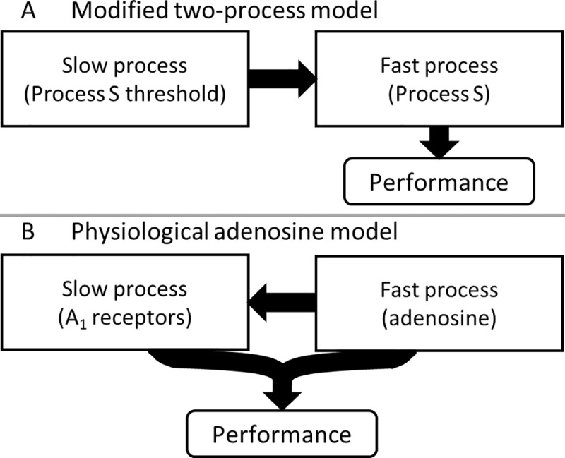
Mathematical structure of (A) previous mathematical models based on the two-process model, and (B) the physiologically based adenosine model developed here. Arrows show functional dependences between model variables.
A further important mathematical distinction exists between our model and the prior McCauley et al. model. Whereas our model’s dynamics are always convergent, the McCauley et al. model’s predictions are divergent in the long-time limit for sleep durations shorter than a critical duration [17]. This feature of convergence improves the McCauley et al. model’s performance on schedules that involve very short sleep opportunities (<4 h), which is one condition in which our model should next be tested. In a physiological context, we expect dynamics to converge, since it is unclear how to physiologically interpret divergence. The PVT output of our model is also a bounded function (sigmoid) of the physiological variables, implying a ceiling for performance impairment, reflective of the fact that there is a theoretical limit on the number of possible lapses per test. We note that our model is similar in the long-time limit to a previous phenomenological approach that assumed a ceiling on lapse probability [46]; one difference being that our model output is total number of lapses per test rather than lapse probability per trial. While our model is designed to test a hypothesis related to the adenosine system, there are many other important sleep-promoting molecules in the brain. These include cytokines, nitric oxide, and prostaglandins. As more data come to light, it may be necessary to extend our model to include other ligand/receptor systems and potential interactions between these systems. A sensible next step would be modeling the dynamics of A2A receptors, which are involved in mediating effects of caffeine [47]. Previously we developed a physiological model of the neuronal systems that regulate sleep and alertness [32], including the effects of caffeine on subjective alertness and sleep [48]. The effects of caffeine were also recently included in another model of cognitive performance [49]. Both these models of caffeine, however, currently use a sleep homeostatic process that is not directly linked to adenosine receptor dynamics [50]. Integrating neuronal sleep models with the adenosine system model developed here is therefore an important future goal with multiple applications.
In experiments involving rodents, there is some evidence of an allostatic response to chronic sleep restriction, meaning the homeostatic set-point may change in response to chronic sleep restriction. Specifically, EEG slow-wave activity in male F344 rats is increased by sleep restriction on the first day, but this elevation disappears as sleep restriction continued on days 2–5. Moreover, when the animals recover, slow-wave activity falls below baseline levels [51]. Such a response could be explained by a decrease in the rate of adenosine production [52]. The existence of an allostatic response is, however, disputed. Leemburg et al. [53] found slow-wave activity was consistently elevated during both sleep restriction and recovery in male WHY rats, although this conflict could be due to strain differences. A decrease in slow-wave activity during chronic sleep restriction has not been reported in humans, but slow-wave activity notably shows little to no change during chronic sleep restriction, despite declining cognitive performance [4]. This outcome could be explained by different receptors mediating different functions (slow-wave activity vs. cognitive performance) and responding differently to sleep restriction. Indeed, there is evidence of A2A receptor down-regulation in some brain regions following sleep deprivation [30]. This would be consistent with the finding that selective A2A agonists promote non-rapid-eye-movement sleep, while selective A1 agonists do not [54]. However, there is significant functional overlap between receptor types, since A1 receptors also mediate slow-wave activity changes in response to sleep restriction [43], so it cannot be as simple as A1 receptors controlling cognitive performance and A2A receptors controlling slow-wave activity; a more complex model is needed.
Our model has limitations and raises new questions. We have tested the model against two datasets, but in each case, we used group-average data, similar to other chronic sleep restriction models in their initial development [17,18]. Accounting for individual differences is particularly valuable, given large and stable differences between individuals in their vulnerability to sleep restriction on specific tasks [55,56]. Ramakrishnan et al. recently reported fitting a two-process-based model on an individual basis, but only after excluding the 3 most variable participants from a sample of 18 [57]. Since our model is based on underlying physiology, it could potentially be used to identify candidate mechanisms that account for individual differences. Ultimately, these mechanisms could be empirically tested using adenosine receptor imaging techniques [58].
In summary, we present the basis for a new model that is the first to explicitly and quantitatively link the sleep homeostatic process, cognitive performance, and sleep patterns to an underlying physiological and molecular biological mechanism. Although we are constrained by physiology in posing this model and fitting its parameter values, it performs similarly to the best existing phenomenological ad hoc models for PVT performance, which are free of such constraints. In addition, it advances beyond most of these models in accurately predicting sleep. The model could therefore be used to generate one-step predictions of both sleep and performance, rather than common two-step approaches in which sleep patterns are first derived and performance then predicted [59]. Our findings provide a physiologically plausible basis for observed changes in cognitive performance and sleep under a variety of experimental conditions. Critically, our model’s structure sheds light on the potential origin of empirical observations that sleep homeostasis involves dynamics on both short and long time scales.
Acknowledgments
The authors thank OJ Walch, D Elmenhorst, EM Elmenhorst, MA St. Hilaire, and DA Dean II for their helpful comments.
Data Availability
All code for the model presented in this paper is available through GitHub at the URL https://github.com/ajkphillips/CSR.
Funding Statement
This work was supported by the National Space Biomedical Research Institute through NASA NCC 9-58 to AJKP (PF02101 and HFP01701) and EBK (HFP01604 and HFP02802); the National Institutes of Health to AJKP (K99HL119618, R00HL119618) and EBK (P01-AG009975, RC2-HL101340, R01HL114088, K02-HD045459, and K24-HL105664), and the Air Force Office of Scientific Research to EBK (FA9550-06-0080/O5NL132). The funders had no role in study design, data collection and analysis, decision to publish, or preparation of the manuscript.
References
- 1.Jewett ME, Dijk DJ, Kronauer RE, Dinges DF. Dose-response relationship between sleep duration and human psychomotor vigilance and subjective alertness. Sleep. 1999; 22: 171–179. [DOI] [PubMed] [Google Scholar]
- 2.Drummond SPA, Paulus MP, Tapert SF. Effects of two nights sleep deprivation and two nights recovery sleep on response inhibition. J Sleep Res. 2006; 15: 261–265. doi: 10.1111/j.1365-2869.2006.00535.x [DOI] [PubMed] [Google Scholar]
- 3.Cohen DA, Wang W, Wyatt JK, Kronauer RE, Dijk DJ, Czeisler CA, et al. Uncovering residual effects of chronic sleep loss on human performance. Sci Trans Med. 2010; 2: 14ra3. [DOI] [PMC free article] [PubMed] [Google Scholar]
- 4.Van Dongen HPA, Maislin G, Mullington JM, Dinges DF. The cumulative cost of additional wakefulness: Dose-response effects on neurobehavioral functions and sleep physiology from chronic sleep restriction and total sleep deprivation. Sleep. 2003; 26: 117–126. [DOI] [PubMed] [Google Scholar]
- 5.Belenky G, Wesenstein NJ, Thorne DR, Thomas ML, Sing HC, Redmond DP, et al. Patterns of performance degradation and restoration during sleep restriction and subsequent recovery: A sleep dose-response study. J Sleep Res. 2003; 12: 1–12. [DOI] [PubMed] [Google Scholar]
- 6.Daan S, Beersma DG, Borbély AA. Timing of human sleep: Recovery process gated by a circadian pacemaker. Am J Physiol. 1984; 246: R161–183. [DOI] [PubMed] [Google Scholar]
- 7.Åkerstedt T, Folkard S. The three-process model of alertness and its extension to performance, sleep latency, and sleep length. Chronbiol Int. 1997; 14: 115–123. [DOI] [PubMed] [Google Scholar]
- 8.Jewett ME, Kronauer RE. Interactive mathematical models of subjective alertness and cognitive throughput in humans. J Biol Rhythms. 1999; 6: 588–597. [DOI] [PubMed] [Google Scholar]
- 9.Achermann P. The two-process model of sleep regulation revisited. Aviat Space Environ Med. 2004;75: A37–A43. [PubMed] [Google Scholar]
- 10.Belyavin AJ, Spencer MB. Modeling performance and alertness: The QinetiQ approach. Aviat Space Environ Med. 2004; 75: A93–A103. [PubMed] [Google Scholar]
- 11.Mallis MM, Mejdal S, Nguyen TT, Dinges DF. Summary of the key features of seven biomathematical models of human fatigue and performance. Aviat Space Environ Med. 2004; 75: A4–A14. [PubMed] [Google Scholar]
- 12.Moore-Ede M, Heitmann A, Guttkuhn R, Trutschel U, Aguirre A, Croke D. Circadian alertness simulator for risk assessment in transportation: Application to reduce frequency and severity of truck accidents. Aviat Space Environ Med. 2004; 75: A107–A118. [PubMed] [Google Scholar]
- 13.Van Dongen HPA, Rogers NL, Dinges DF. Sleep debt: Theoretical and empirical issues. Sleep Biol Rhythms. 2003; 1: 5–13. [Google Scholar]
- 14.Van Dongen HPA. Comparison of mathematical model predictions to experimental data of fatigue and performance. Aviat Space Environ Med. 2004; 75: A15–A36. [PubMed] [Google Scholar]
- 15.Hursh SR, Redmond DP, Johnson ML, Thorne DR, Belenky G, Balkin TJ, et al. Fatigue models for applied research in warfighting. Aviat Space Environ Med. 2004; 75: A44–A53. [PubMed] [Google Scholar]
- 16.Johnson ML, Belenky G, Redmond DP, Thorne DR, Williams JD, Hursh SR, et al. Modulating the homeostatic process to predict performance during chronic sleep restriction. Aviat Space Environ Med. 2004; 75: A141–A146. [PubMed] [Google Scholar]
- 17.McCauley P, Kalachev LV, Smith AD, Belenky G, Dinges DF, Van Dongen HPA. A new mathematical model for the homeostatic effects of sleep loss on neurobehavioral performance. J Theor Biol. 2009; 256: 227–239. doi: 10.1016/j.jtbi.2008.09.012 [DOI] [PMC free article] [PubMed] [Google Scholar]
- 18.Rajdev P, Thorsley D, Rajaraman S, Rupp TL, Wesensten NJ, Balkin TJ, et al. A unified mathematical model to quantify performance impairment for both chronic sleep restriction and total sleep deprivation. J Theor Biol. 2013; 331:66–77. doi: 10.1016/j.jtbi.2013.04.013 [DOI] [PubMed] [Google Scholar]
- 19.Porkka-Heiskanen T, Strecker RE, McCarley RW. Brain site-specificity of extracellular adenosine concentration changes during sleep deprivation and spontaneous sleep: An in vivo microdialysis study. Neuroscience. 2000; 99: 507–517. [DOI] [PubMed] [Google Scholar]
- 20.Basheer R, Bauer A, Elmenhorst D, Ramesh V, McCarley RW. Sleep deprivation upregulates A1 adenosine receptors in the rat basal forebrain. Neuroreport. 2007; 18: 1895–1899. doi: 10.1097/WNR.0b013e3282f262f6 [DOI] [PubMed] [Google Scholar]
- 21.Kim Y, Bolortuya Y, Chen L, Basheer R, McCarley RW, Strecker RE. Decoupling of sleepiness from sleep time and intensity during chronic sleep restriction: Evidence for a role of the adenosine system. Sleep. 2012; 35: 861–869. doi: 10.5665/sleep.1890 [DOI] [PMC free article] [PubMed] [Google Scholar]
- 22.Van Dongen HPA, Belenky G, Krueger JM. A local, bottom-up perspective on sleep deprivation and neurobehavioral performance. Curr Top Med Chem. 2011; 11: 2414–2422. [DOI] [PMC free article] [PubMed] [Google Scholar]
- 23.National Sleep Foundation. How much sleep do we really need? 2016. Available from: http://sleepfoundation.org/how-sleep-works/how-much-sleep-do-we-really-need
- 24.Mitler MM, Carskadon MA, Czeisler CA, Dement WC, Dinges DF, Graeber RC. Catastrophes, sleep, and public policy: Consensus report. Sleep. 1988; 11: 100–109. [DOI] [PMC free article] [PubMed] [Google Scholar]
- 25.Basheer R, Strecker RE, Thakkar MM, McCarley RW. Adenosine and sleep-wake regulation. Prog Neurobiol. 2004; 73: 379–396. doi: 10.1016/j.pneurobio.2004.06.004 [DOI] [PubMed] [Google Scholar]
- 26.Phillips AJK, Robinson PA, Kedziora DJ, Abeysuriya RG. Mammalian sleep dynamics: How diverse features arise from a common physiological framework. PLoS Comput Biol. 2010; 24: e1000826. [DOI] [PMC free article] [PubMed] [Google Scholar]
- 27.Buchsbaum MS, Gillin JC, Wu J, Hazlett E, Sicotte N, Dupont RM, et al. Regional cerebral glucose metabolic rate in human sleep assessed by positron emission tomography. Life Sciences. 1989; 45: 1349–1356. [DOI] [PubMed] [Google Scholar]
- 28.Xie L, Kang H, Xu Q, Chen MJ, Liao Y, Thiyagarajan M, et al. Sleep drives metabolite clearance from the adult brain. Science. 2013; 342: 373–377. doi: 10.1126/science.1241224 [DOI] [PMC free article] [PubMed] [Google Scholar]
- 29.Dunwiddie TV, Masino SA. The role and regulation of adenosine in the central nervous system. Ann Rev Neurosci. 2001; 24: 31–55. doi: 10.1146/annurev.neuro.24.1.31 [DOI] [PubMed] [Google Scholar]
- 30.Basheer R, Halldner L, Alanko L, McCarley RW, Fredholm BB, Porkka-Heiskanen T. Opposite changes in adenosine A1 and A2A receptor mRNA in the rat following sleep deprivation. Neuroreport. 2001; 12: 1577–1580. [DOI] [PubMed] [Google Scholar]
- 31.Imeri L, Opp MR. How (and why) the immune system makes us sleep. Nature Rev Neurosci. 2009; 10: 199–210. [DOI] [PMC free article] [PubMed] [Google Scholar]
- 32.Fulcher BD, Phillips AJK, Robinson PA. Quantitative physiologically based modeling of subjective fatigue during sleep deprivation. J Theor Biol. 2010; 264: 407–419 doi: 10.1016/j.jtbi.2010.02.028 [DOI] [PubMed] [Google Scholar]
- 33.Phillips AJK, Chen PY, Robinson PA. Probing the mechanisms of chronotype using quantitative modeling. J Biol Rhythms. 2010; 25: 217–227. doi: 10.1177/0748730410369208 [DOI] [PubMed] [Google Scholar]
- 34.Dijk DJ, Czeisler CA. Contribution of the circadian pacemaker and the sleep homeostat to sleep propensity, sleep structure, electroencephalographic slow waves, and sleep spindle activity in humans. J Neurosci. 1995; 15: 3526–3538. [DOI] [PMC free article] [PubMed] [Google Scholar]
- 35.Van Dongen HPA, Dinges DF. Investigating the interaction between the homeostatic and circadian processes of sleep-wake regulation for the prediction of waking neurobehavioural performance. J Sleep Res. 2003; 12:181–187. [DOI] [PubMed] [Google Scholar]
- 36.McCauley P, Kalachev LV, Mollicone DJ, Banks S, Dinges DF, Van Dongen HPA. Dynamic circadian modulation in a biomathematical model for the effects of sleep and sleep loss on waking neurobehavioral performance. Sleep. 2013; 36: 1987–1997. doi: 10.5665/sleep.3246 [DOI] [PMC free article] [PubMed] [Google Scholar]
- 37.Cronstein BN, Rosenstein ED, Kramer SB, Weissmann G, Hirschhorn R. Adenosine; a physiologic modulator of superoxide anion generation by human neutrophils. Adenosine acts via an A2 receptor on human neutrophils. J Immunol. 1985; 135: 1366–1371. [PubMed] [Google Scholar]
- 38.Fastbom J, Pazos A, Probst A, Palacios JM. Adenosine A1 receptors in the human brain: A quantitative autoradiographic study. 1987; 22: 827–839. [DOI] [PubMed] [Google Scholar]
- 39.Lim J, Dinges DF. Sleep deprivation and vigilant attention. Ann NY Acad. Sci. 2008; 1129: 305–322. doi: 10.1196/annals.1417.002 [DOI] [PubMed] [Google Scholar]
- 40.Wehr TA, Mould DE, Barbato GI, Giesen HA, Siedel JA, Barker CH, Bender CH. Conservation of photoperiodic-responsive mechanisms in humans. Am J Physiol. 1993; 265: R846–R857. [DOI] [PubMed] [Google Scholar]
- 41.Ekirch AR. Segmented sleep in preindustrial societies. Sleep. 2016; 39: 715–716. doi: 10.5665/sleep.5558 [DOI] [PMC free article] [PubMed] [Google Scholar]
- 42.Phillips AJK, Fulcher BD, Robinson PA, Klerman EB. Mammalian rest/activity patterns explained by physiologically based modeling. PLoS Comput Biol. 2013; 9: e1003213 doi: 10.1371/journal.pcbi.1003213 [DOI] [PMC free article] [PubMed] [Google Scholar]
- 43.Bjorness TE, Kelly CL, Gao T, Poffenberger V, Greene RW. Control and function of the homeostatic sleep response by adenosine A1 receptors. J Neurosci. 2009; 29: 1267–1276. doi: 10.1523/JNEUROSCI.2942-08.2009 [DOI] [PMC free article] [PubMed] [Google Scholar]
- 44.Landolt HP. Sleep homeostasis: A role for adenosine in humans? Biochem Pharmacol. 2008; 75: 2070–2079. doi: 10.1016/j.bcp.2008.02.024 [DOI] [PubMed] [Google Scholar]
- 45.St Hilaire MA, Rüger M, Fratelli F, Hull JT, Phillips AJ, Lockley SW. Modeling neurocognitive decline and recovery during repeated cycles of extended sleep and chronic sleep deficiency. Sleep. 2016; 14: zsw009. [DOI] [PMC free article] [PubMed] [Google Scholar]
- 46.Olofsen E, Van Dongen HPA, Mott CG, Balkin TJ, Terman D. Current approaches and challenges to development of an individualized sleep and performance prediction model. Open Sleep J. 2010; 3: 24–43. [Google Scholar]
- 47.Huang ZL, Qu WM, Eguchi N, Schwarzschild MA, Fredholm BB, Urade Y, Hayaishi O. Adenosine A2A, but not A1, receptors mediate the arousal effect of caffeine. Nat Neurosci. 2005; 8: 858–859. doi: 10.1038/nn1491 [DOI] [PubMed] [Google Scholar]
- 48.Puckeridge M, Fulcher BD, Phillips AJK, Robinson PA. Incorporation of caffeine into a quantitative model of fatigue and sleep. J Theor Biol. 2011; 273: 44–54. doi: 10.1016/j.jtbi.2010.12.018 [DOI] [PubMed] [Google Scholar]
- 49.Ramakrishnan S, Rajaraman S, Laxminarayan S, Wesensten NJ, Kamimori GH, Balkin TJ, Reifman J. A biomathematical model of the restoring effects of caffeine on cognitive performance during sleep deprivation. J Theor Biol. 2013; 319: 23–33. doi: 10.1016/j.jtbi.2012.11.015 [DOI] [PubMed] [Google Scholar]
- 50.Fulcher BD, Phillips AJK, Postnova S, Robinson PA. A physiologically based model of orexinergic stabilization of sleep and wake. PLoS One. 2–14; 9: e91982 doi: 10.1371/journal.pone.0091982 [DOI] [PMC free article] [PubMed] [Google Scholar]
- 51.Kim Y, Laposky AD, Bergmann BM, Turek FW. Repeated sleep restriction in rats leads to homeostatic and allostatic responses during recovery sleep. Proc Natl Acad Sci USA. 2007; 104:10697–10702. doi: 10.1073/pnas.0610351104 [DOI] [PMC free article] [PubMed] [Google Scholar]
- 52.Clasadonte J, McIver SR, Schmitt LI, Halassa MM, Haydon PG. Chronic sleep restriction disrupts sleep homeostasis and behavioral sensitivity to alcohol by reducing the extracellular accumulation of adenosine. J Neurosci. 2014; 34: 1879–1891. doi: 10.1523/JNEUROSCI.2870-12.2014 [DOI] [PMC free article] [PubMed] [Google Scholar]
- 53.Leemburg S, Vyazovskiy VV, Olcese U, Bassetti CL, Tononi G, Cirelli C. Sleep homeostasis in the rat is preserved during chronic sleep restriction. Proc Natl Acad Sci USA. 2010; 7: 15939–15944. [DOI] [PMC free article] [PubMed] [Google Scholar]
- 54.Satoh S, Matsumura H, Hayaishi O. Involvement of adenosine A2A receptor in sleep promotion. Eur J Pharm. 1998; 351: 155–162. [DOI] [PubMed] [Google Scholar]
- 55.Van Dongen HPA, Baynard MD, Maislin G, Dinges DF. Systematic interindividual differences in neurobehavioral impairment from sleep loss: Evidence of trait-like differential vulnerability. Sleep. 2004; 27: 423–433. [PubMed] [Google Scholar]
- 56.Rupp TL, Wesensten NJ, Balkin TJ. Trait-like vulnerability to total and partial sleep loss. Sleep. 2012; 35: 1163–1172. doi: 10.5665/sleep.2010 [DOI] [PMC free article] [PubMed] [Google Scholar]
- 57.Ramakrishnan S, Lu W, Laxminarayan S, Wesensten NJ, Rupp TL, Balkin TJ, Reifman J. Can a mathematical model predict an individual’s trait-like response to both total and partial sleep loss? J Sleep Res. 2015; 24: 262–269. doi: 10.1111/jsr.12272 [DOI] [PubMed] [Google Scholar]
- 58.Elmenhorst D, Meyer PT, Winz OH, Matusch A, Ermert J, Coenen HH, et al. Sleep deprivation increases A1 adenosine receptor binding in the human brain: A positron emission tomography study. J Neurosci. 2007; 27: 2410–2415. doi: 10.1523/JNEUROSCI.5066-06.2007 [DOI] [PMC free article] [PubMed] [Google Scholar]
- 59.Hursh SR, Van Dongen HPA. Fatigue and performance modeling In: Krieger MH, Roth T, Dement WC. Principles and practice of sleep medicine, 5th ed. St. Louis, MO: Elsevier Saunders; 2010. pp. 745–752. [Google Scholar]
Associated Data
This section collects any data citations, data availability statements, or supplementary materials included in this article.
Data Availability Statement
All code for the model presented in this paper is available through GitHub at the URL https://github.com/ajkphillips/CSR.