Modeling continuous response variables using ordinal regression

Abstract

We study the application of a widely used ordinal regression model, the cumulative probability model (CPM), for continuous outcomes. Such models are attractive for the analysis of continuous response variables because they are invariant to any monotonic transformation of the outcome and because they directly model the cumulative distribution function from which summaries such as expectations and quantiles can easily be derived. Such models can also readily handle mixed type distributions. We describe the motivation, estimation, inference, model assumptions, and diagnostics. We demonstrate that CPMs applied to continuous outcomes are semiparametric transformation models. Extensive simulations are performed to investigate the finite sample performance of these models. We find that properly specified CPMs generally have good finite sample performance with moderate sample sizes, but that bias may occur when the sample size is small. CPMs are fairly robust to minor or moderate link function misspecification in our simulations. For certain purposes, the CPM are more efficient than other models. We illustrate their application, with model diagnostics, in a study of the treatment of HIV. CD4 cell count and viral load 6 months after the initiation of antiretroviral therapy are modeled using CPMs; both variables typically require transformations and viral load has a large proportion of measurements below a detection limit.

1. Introduction

Continuous data are also ordinal, and ordinal regression models can be fit to continuous outcomes [1, 2]. The first ordinal regression model was developed by Walker & Duncan [3] as an extension of logistic regression to ordered categorical data. This class of models was later studied by McCullagh [4] and referred to as proportional odds models for the logit link and proportional hazards models for the complementary log-log link (cloglog). To distinguish this class of models from other ordinal regression models (e.g., continuation ratio models [5, 6], adjacent-categories models [7, 8], and ordinal stereotype models [9]), these models have been referred to as cumulative link models [10]. However, this nomenclature is problematic because probabilities, not link functions, are added. Hence, we refer to this class of models as cumulative probability models (CPMs).

The use of ordinal CPMs for continuous outcomes has many attractive features. First, ordinal regression models are robust because they only incorporate the order information of response variables and are therefore invariant to any monotonic transformation of outcomes. This is particularly useful when the distributions of continuous responses are skewed and different transformations may give conflicting results. Second, CPMs directly model the conditional cumulative distribution function (CDF), from which other components of the conditional distribution (e.g., mean and quantiles) can be easily derived. Therefore, one can examine various aspects of the conditional distribution from a single CPM, whereas other regression models often only focus on one aspect. Finally, CPMs can handle any orderable response, including those with mixed types of continuous and discrete ordinal distributions. This may be particularly useful when dealing with detection limits, e.g., measurements censored at an assay detection limit resulting in a mixture of an undetectable category and detectable quantities.

Although the idea of using ordinal CPMs for continuous outcomes is attractive and has been around for a while, we have not seen it used very often in practice. This may be in part due to computing limitations, as most software that fit CPMs are currently designed for ordered categorical outcomes with relatively small numbers of possible response values, and hence a small number of intercepts. This need not be the case anymore. With modern computing power and improved algorithms, software capitalizing on the sparse information matrix of CPMs can handle thousands of intercepts [1, 11], as will be demonstrated below. However, we believe the primary reason for limited use of these models with continuous outcomes is a lack of awareness. CPMs were first invented to handle discrete ordinal outcomes, and their potential utility for the analysis of continuous outcomes has been largely unrecognized. Furthermore, we are unaware of any in-depth study of the use of CPMs for continuous outcomes.

The goal of this manuscript is to describe and study the application of CPMs to continuous outcomes. In Section 2 we describe details of the approach including the motivation, estimation, inference, assumptions and model diagnostics. In particular, we motivate the use of semiparametric transformation models for continuous outcomes and show how they lead to CPMs. In Section 3, we investigate the finite sample performance of CPMs with and without proper link function specification through simulations. In Section 4, we illustrate their application to an HIV study modelling CD4 cell count and viral load 6 months after the initiation of antiretroviral therapy. Both variables typically require transformations and viral load has a large proportion of measurements below a detection limit. Section 5 contains a discussion. Additional simulation results are given in Supplemental Materials. R code for all simulations and analyses is posted at http://biostat.mc.vanderbilt.edu/ArchivedAnalyses.

2. Cumulative Probability Models for Continuous Outcomes

2.1. Motivation

Regression analyses of continuous outcomes often require an assumption on the outcome distribution or a transformation of the outcome so that it is more amenable for analysis. Because the correct transformation is often unknown, it is desirable to model the relative positions of the outcome values instead of picking a transformation. In addition, it would be appealing to estimate the outcome distribution instead of assuming it.

One approach to achieving these goals is to model the observed outcome Y as a monotonic transformation of a latent variable Y^∗, Y = H(Y^∗), where the function H(·) is strictly increasing but unknown otherwise (the “strictly” part will be relaxed later) and Y^∗ = β^T X + ε, with β^TX a linear combination of the input variables X and ε ~ F_ε, where F_ε is a specified distribution. The intercept is unnecessary in Y^∗ = β^TX + ε because a shift can be reflected in the transformation H(·). This approach leads to the linear transformation model,

$$Y=H\left({\beta }^{T}X+\epsilon \right),\text{where}\epsilon ~F_{\epsilon }.$$ (1)

This model is semi-parametric because the effect of X is modeled parametrically while the functional form of H(·) is unspecified. The model has been studied by others, including Zeng & Lin [12]. The cumulative probability function of Y conditional on X can be written as

$$F\left(y|X\right)=P\left(Y\le y|X\right)=P\left[H\left({\beta }^{T}X+\epsilon \right)\le y|X\right]=P\left[\epsilon \le H^{-1}\left(y\right)-{\beta }^{T}X|X\right]=F_{\epsilon }\left[H^{-1}\left(y\right)-{\beta }^{T}X\right].$$

For simplicity, let $G=F_{\epsilon }^{-1}$ and α = H⁻¹. Then, we have

$$G\left[P\left(Y\le y|X\right)\right]=\alpha \left(y\right)-{\beta }^{T}X,$$ (2)

where G(·) is a link function and α(·) is an intercept function. In other words, the linear transformation model (1) is also a CPM (2). When focused on the observed values {y_i; i = 1, …, n}, the CPM can be expressed as

$$G[P(Y\le y_i|X)]={\alpha }_i-{\beta }^{T}X,$$ (3)

where α_i = α(y_i) for i = 1, ⋯ , n. Here the parameters are (β, α₁, …, α_n). Without loss of generality, we assume y₁ ≤ ⋯ ≤ y_n. Since α⁻¹(·) is increasing, we have the constraint α₁ ≤ … ≤ α_n, and α_i = α_j whenever y_i = y_j.

The above derivation also works when H(·) is increasing but not strictly increasing. For mathematical clarity, we assume H(·) is left continuous and define H⁻¹(y) = sup{z : H(z) ≤ y}. It can be shown that H(H⁻¹(y)) ≤ y, and that H(z) ≤ y if and only if z ≤ H⁻¹(y). In practice, the direction of the continuity of H() does not matter as long as Y^∗ follows a continuous distribution. If H(·) is constant on an interval, the observed response variable Y can be a mixed type of continuous and discrete ordinal variables. In the extreme case where H() is a step function, Y is a discrete ordinal variable. Therefore, the linear transformation model (1) and the associated CPM (2) can be used to model continuous, discrete ordinal, and mixed types of ordinal and continuous variables.

The CPM (2) has several nice properties. Unlike other commonly used continuous regression models which only focus on one aspect of the conditional distribution, e.g., the conditional mean for linear regression models or a conditional quantile for quantile regression models, the entire conditional distribution is modeled by the CPM. Since α⁻¹(y) = G[P (Y ≤ y|X = 0)], the intercept function α⁻¹() is the link function transformed CDF at baseline X = 0. The intercept function is also the transformation needed for Y such that Y^∗ = α⁻¹ (Y) can be fit with a linear regression model (with error term ε ~ G⁻¹). The association between Y and X is captured by β: a positive β_j means that with the values for all other X variables fixed, an increase in X_j is associated with a stochastic increase in the distribution of Y. As shown in Figure 1, CPMs have an assumption of parallelism. That is, the difference between link function transformed conditional CDFs for different values of covariates is constant, i.e., $G[F_{Y|X=x_2}\left(y\right)]-G[F_{Y|X=x_1}\left(y\right)]=-{\beta }^T\left(x_2-x_1\right),$ which is free of y. Depending on the link function chosen, β can have a nice interpretation, e.g., as a log-odds ratio if G is the logit link function or as a log-hazard ratio if G is the cloglog link function. Table 1 summarizes commonly used link functions, G, and their corresponding error distributions, F_ε, in the transformation model.

Figure 1.

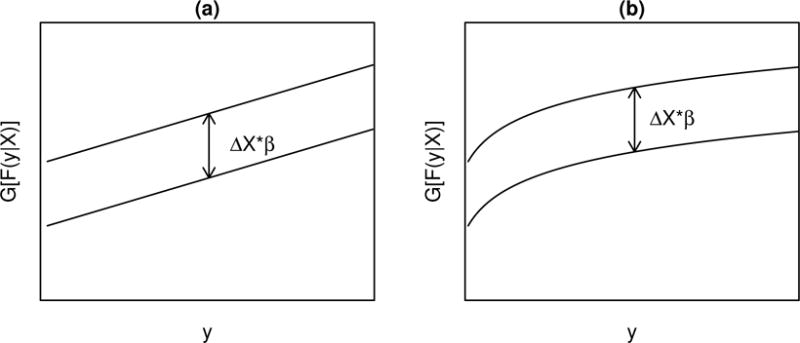
The parallelism assumptions in (a) the normal linear regression model Y = βX + ε with ε ~ N(0, 1) and (b) transformation models Y = H(βX + ε) with ε ~ F_ε, $G=F_{\epsilon }^{-1}$. Adapted from Harrell [2].

Table 1.

Commonly used link functions and their corresponding error distributions.

Name	Link Function	Error Distribution	CDF
logit	log [p/(1 − p)]	logistic	exp (y)/[1 + exp (y)]
probit	Φ−1(p)	normal	Φ(y)
loglog	−log [− log (p)]	extreme value type II (Gumbel Maximum)	exp [− exp (−y)]
cloglog	log [− log (1 − p)]	extreme value type I (Gumbel Minimum)	1 − exp [− exp (y)]

Φ(·) is the CDF of the standard normal distribution.

When expressed at the observed values {y_i}, the model (3) is very similar to the traditionally defined CPM for ordinal outcomes. In fact, the latter can be viewed as a special case of the linear transformation model. For an ordinal outcome Y with K categories (denoted as C₁, C₂, …, C_K in ascending order), a CPM is traditionally defined as

$$G\left[P\left(Y\le C_k|X\right)\right]={\alpha }_k-{\beta }^{T}X\left(k=1,\dots ,K-1\right),$$

where G is a link function [4, 10]. It is well known that this model is equivalent to having an underlying continuous variable Y^∗ from a linear model Y^∗ = β^T X + ε, where ε ~ F_ε = G⁻¹ and then generating the observed outcome Y^∗, i.e., Y = H (Y^*) = C_j when α_{j − 1} < Y^* ≤ α_j, where −∝ = α₀ < α₁ < … < α_{K − 1} < α_K = +∞. Here H(·) is a left-continuous non-decreasing step function.

2.2. Nonparametric Maximum Likelihood Estimation

We now describe an approximate nonparametric likelihood function for the CPM (3). The nonparametric likelihood for the outcome values is $L\left(\beta ,\alpha \right)={\displaystyle {\prod }_{i=1}^n[F(y_i|x_i)-F(y_i-|x_i)]},$ where $F\left(y-|x\right)={\lim }_{t\uparrow y}{F}^{\ast }\left(t|x\right)$. We approximate this likelihood by replacing F (y_i − |x_i) with F (y_i−1|x_i); this approximation is good when the outcome values are densely placed. Therefore, the nonparametric likelihood is approximately

$$L^{\ast }\left(\beta ,\alpha \right)={\displaystyle \prod _{i=1}^n\left[G^{-1}\left({\alpha }_i-{\beta }^T{x}_i\right)-G^{-1}\left({\alpha }_{i-1}-{\beta }^T{x}_i\right)\right].}$$

Here we added an auxiliary parameter α₀ (< α₁). The NPMLEs can be obtained by maximizing L^∗(β, α). Since α₀ and α_n are only present in the first and the last terms of L^∗, respectively, and also since G⁻¹ is a monotonic increasing function, L^∗ is maximized when ${\widehat{\alpha }}_0=-\infty$ and ${\widehat{\alpha }}_n=+\infty$. Plugging in ${\widehat{\alpha }}_0$ and ${\widehat{\alpha }}_n$, L^∗(β, α) can be simplified as

$$\left[G^{-1}\left({\alpha }_1-{\beta }^T{x}_1\right)\right]{\displaystyle \prod _{i=2}^{n-1}\left[G^{-1}\left({\alpha }_i-{\beta }^T{x}_i\right)-G^{-1}\left({\alpha }_{i-1}-{\beta }^T{x}_i\right)\right]}\cdot \left[1-G^{-1}\left({\alpha }_{n-1}-{\beta }^T{x}_n\right)\right].$$ (4)

We maximize (4) to obtain the NPMLE for β and (α₁, …, α_n−1).

Note that (4) has the same structure as the multinomial likelihood of the CPM for a discrete outcome variable with only one observation in each category. Therefore, maximizing (4) can be easily achieved by treating Y as a discrete variable and fitting the discrete CPM using standard statistical software. Although this is convenient in practice, computational challenges arise with large sample sizes because the Newton-Raphson algorithm typically used for maximization requires inverting the Hessian matrix whose dimensions ((n − 1 + p) × (n − 1 + p) when there are no ties) tend to increase with the sample size. However, as shown in Figure 2, due to the special – structure of the likelihood function (4), the portion of the Hessian matrix with respect to the intercepts is tridiagonal. This structure allows matrix inversion efficiently through Cholesky decomposition [1]. Taking advantage of these facts, Harrell implemented a computationally efficient algorithm to obtain the NPMLE with the orm() function in the rms package [11] in R software [13].

Figure 2.

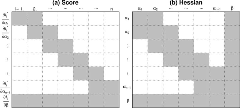
(a) Each observation’s contribution to the score function assuming observations are ordered by the value of y, i.e., y₁ < y₂ < ⋯ < y_n. White region indicates zero and grey region indicates non-zero values. (b) The bordered tridiagonal structure of Hessian matrix of log(L^∗) with respect to intercepts and slopes. Since α_i = α_j whenever y_i = y_j, the score function and Hessian matrix have similar forms when there are ties in the outcome.

We note that the orm() function assumes a slightly different model formulation, $G_1\left[1-F\left(y|X\right)\right]={\alpha }_{\mathit{orm}}\left(y\right)+{\beta }_{\mathit{orm}}X.$ This formulation is equivalent to (3) if we define G(t) = −G₁(1 − t), α = −α_orm and β = β_orm. Therefore, to fit model (3) using the orm() function, for symmetric error distributions such as normal and logistic distributions, since G(t) = −G(1 − t), the same link function can be used in orm() and the regression coefficients α_orm differ from α in (3) only by sign. For non-symmetric error distributions with a link function G (e.g., G is cloglog or loglog), we specify its complementary version G₁(t) = −G(1 − t) as the link function in orm() (e.g., G₁ is loglog or cloglog, respectively).

Once we have the NPMLE $\left(\widehat{\beta },\widehat{\alpha }\right)$_, the conditional CDF, F (y|X), can be estimated at {y₁, …, y_n}: $\widehat{F}(y_i|X)=G^{-1}({\widehat{\alpha }}_i-\widehat{\beta }X)$. The entire conditional CDF can be approximated using a step function connecting $\widehat{F}(y_i|X)$; corresponding distribution is discrete with probability at y_i being $\widehat{f}(y_i|X)=\widehat{F}(y_i|X)-\widehat{F}(y_{i-1}|X)$ when i > 1 and $\widehat{f}(y_1|X)=\widehat{F}(y_1|X)$. With the estimated CDF, some properties of the conditional distribution can be easily derived. For example, we can estimate the conditional mean as $\widehat{E}(Y|X)={\displaystyle {\sum }_{i=1}^n{y}_1\widehat{f}}(y_i|X)$. With the estimated variance-covariance matrix for $\left(\widehat{\beta },\widehat{\alpha }\right)$_, the standard errors for $\widehat{F}(y_i|X)$ and $\widehat{E}(Y|X)$ can be obtained by the delta method [14]. Figure 3(a) shows an example of an estimated conditional CDF and its pointwise 95% confidence interval. Also, as illustrated in Figure 3(b), the conditional quantiles and their confidence intervals can be obtained from linear interpolation of the inverse of the conditional CDF and its pointwise confidence intervals, respectively.

Figure 3.

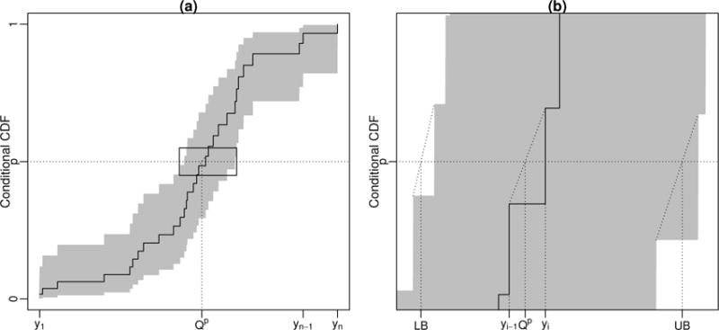
(a): An estimated conditional CDF and its pointwise confidence intervals. (b): An illustration for estimating the p-th quantile of the conditional distribution, denoted as Q^p, and its confidence interval (LB, UB) through linear interpolation between y_i−1 and y_i, where $y_{\mathrm{i}}=\inf \left\{y:\widehat{F}\left(y|X\right)\ge p\right\}$, based on the estimated conditional CDF and its pointwise confidence intervals.

It should be noted that there is no general theory for the asymptotic properties of NPMLEs. Zeng & Lin [12] studied these types of semiparametric transformation models. They only proved the consistency, asymptotic normality, and asymptotic efficiency for censored data and their proofs rely on the boundedness of the estimator of H(·). Based on personal communication, these authors have been working on establishing the asymptotic properties of NPMLEs for semiparametric transformation models with uncensored data [12]. However, for a general continuous response, both the true value of H(·) and its estimator can be unbounded. This imposes tremendous technical difficulties in the proofs. In this manuscript we do not attempt to fill this gap in the theory. Instead, we rely on the facts that this approach is fully likelihood-based and that the effective degrees of freedom of the intercepts are small due to order constraints. We bolster this by performing extensive simulations (Section 3 and additional simulations in Supplemental Materials). Our simulations suggest that with proper model specification (i.e., correctly specifying the link function and the mean model, but leaving H(·) unspecified), the NPMLE procedure just described results in consistent, asymptotically normal estimators with well-approximated variance estimates.

2.3. An Illustration

We illustrate CPMs and compare them with nonparametric and parametric models in the following simple example. Consider a single binary covariate X ~ Bernoulli(0.5), the latent response Y^∗ = βX + ε, where β = 1 and ε ~ N(0, 1), and the observable response Y = H(Y^∗). For simplicity, we set H(y) = y, that is, no transformation is needed. We order the observations so that y₁ < y₂ < … < y_n. In this setting, since the covariate is binary, both nonparametric and parametric models can be easily applied to estimate the conditional CDF. Nonparametrically, we can compute the empirical CDFs for the subgroup X = 0 and the subgroup X = 1, respectively. Parametrically, we can fit a linear regression model to estimate the conditional mean and variance, and then calculate the conditional CDF using the cumulative probability function of the normal distribution. The CPM is semiparametric: we use a probit link function, which assumes the data are normally distributed after some monotonic transformation, but leaves this transformation unspecified. Figure 4 shows the estimation of conditional CDFs with these three approaches when the sample size is 10, 100 and 1000, respectively.

Figure 4.

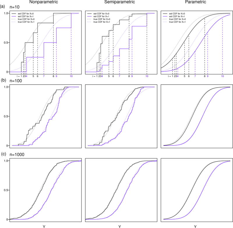
Estimation of conditional CDF from CPMs compared with parametric and nonparametric models in a simple example: (a) with a sample size of 10, (b) with a sample size of 100, and (c) with a sample size of 1000.

The nonparametric approach only uses information from each subgroup to estimate its conditional CDF, i.e., the empirical CDF is a step function with jumps only at the observed values within each subgroup, e.g., 6 jumps for X = 0 and 4 jumps for X = 1 in the specific example with the sample size of 10 in Figure 4 (a). The parametric approach (the normal linear regression model) pools information from all observations and also uses the assumption of a normal error distribution to provide smooth estimates for the conditional CDFs. The CPM (semiparametric) provides something in between, i.e., the estimates are step functions but with jumps at observed values from both subgroups, e.g., 10 jumps for both X = 0 and X = 1 as shown in the middle panel of Figure 4 (a). The nonparametric approach does not make any assumptions about the conditional distributions; therefore, it is the most robust estimation procedure. But it is not efficient because it only uses information within each subgroup and it is not easily extended to continuous or multivariate X. The parametric approach assumes normality for the conditional distribution. It is most efficient if the assumption is correct, but not robust to model misspecification. The CPM does not make full parametric assumptions about the conditional distributions (i.e., it only assumes that after some unspecified transformation, the data are normal), but still pools information by assuming a shared shape for the conditional distributions. Therefore, the CPM provides a compromise between efficiency and robustness.

2.4. Model Diagnostics

As with discrete variables, the link function of CPMs for continuous responses should ideally be pre-specified based on preliminary scientific knowledge and convenience of interpretation. This may be challenging in application since it requires the specification of the error distribution on the unknown transformed scale. Therefore, model diagnostics, especially for the choice of link functions, are important. A goodness-of-link test has been developed by Genter & Farewell to discriminate the model fit between probit, cloglog, and loglog link functions for discrete variables [15]. The main idea is that these three link functions can be considered as special cases of a generalized log-gamma link function with an extra parameter. Then, a likelihood ratio test comparing the full model (using the log-gamma link) with the reduced model (using the probit, cloglog, or loglog link) could provide information about the goodness of fit. To avoid the computational burden of fitting the full model, Genter & Farewell proposed to compare the log-likelihoods of probit, cloglog, and loglog models directly as a conservative approximation to the formal likelihood ratio test [15]. Specifically, they claim that if twice the difference of two log-likelihoods exceeds the appropriate percentile of a chi-square distribution with 1 degree of freedom, one can infer that the link with the smaller likelihood is inappropriate. This approach is also applicable to continuous responses. However, an automated link function selection procedure based on the largest log-likelihood should be used with caution because it seems to share the problems of step-wise selection procedures [16, 17] according to our simulations (see Table S.1 in Supplemental Materials S.1), i.e., type I error rates are inflated, standard error estimates are too small, and the confidence intervals are too narrow.

The model fit of CPMs can also be examined graphically with residuals. As described in Section 2.1, the intercept function α(y) can be interpreted as the best transformation needed to fit a linear model. Therefore, we can transform the observed y_i to $\widehat{\alpha }(y_i)={\widehat{\alpha }}_i$ and explore the model fit with residuals, ${\widehat{\alpha }}_i-{\widehat{\beta }}^T{x}_i$, on the transformed scale. Alternatively, we can use probability-scale residuals, which were originally proposed for discrete ordinal variables [18, 19]. Probability-scale residuals are functions of fitted conditional CDFs. They are approximately uniformly distributed with proper model specification of continuous outcomes, and are therefore particularly useful in this setting. We illustrate the application of this new residual with details in Section 4.

3. Simulation Studies

3.1. With Proper Link Function Specification: Bias, Coverage, and Relative Efficiency

In this section, we first conduct simulations to evaluate the finite sample performance of CPMs for continuous response with proper link function specification. We generated data from Y = exp (β₁X₁ + β₂X₂ +ε), where X₁ ~ Bernoulli(0.5), X₂ ~ N(0, 1), β₁ = 1 and β₂ = −0.5, and with two error distributions: (i) ε ~ N(0, 1) and (ii) ε generated from the extreme value distribution (type I) as in Table 1. The corresponding properly specified link functions for these two error distributions are probit and cloglog, respectively. We conducted simulations for different sample sizes with n = 25, 50, 100, 200, 500, and 1000. For each sample size, simulations were replicated 10, 000 times. For the purpose of better visualization, we summarize the results with figures. More details of simulation results can be found in Supplemental Materials S.2.1.

As discussed in Section 2.1, when the link function is properly specified, the intercept function α(y) of CPMs corresponds to the proper transformation needed for the parametric linear model, which is log (y) in this case. With NPMLE, α(y) is estimated using a step function with jumps at observed values of Y. We plot $\widehat{\alpha }(y)$ versus the proper transformation log(y) from the first simulation replicate with n = 100 in Figure 5. The average of the step function estimates $\widehat{\alpha }(y)$ over all 10, 000 simulation replicates is also plotted. According to Figure 5, in our simulations with sample size of 100, the NPMLE $\widehat{\alpha }(y)$ shows little bias compared with the true transformation except in tail regions, where little information is observed. The range of near agreement between average $\widehat{\alpha }(y)$ and log(y) becomes wider as n increases.

Figure 5.

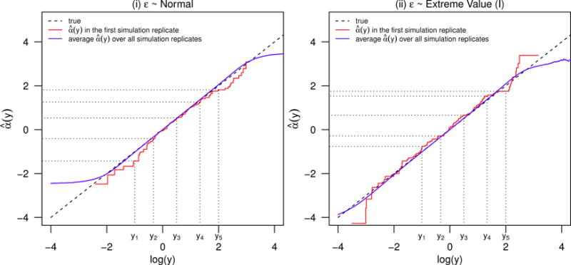
The performance of CPMs on estimating intercepts with n = 100: (i) ε ~ Normal and (ii) ε ~ Extreme Value (I).

Figure 6 summarizes the performance for estimating the regression coefficients, including slopes β₁, β₂, and a few intercept values α(y) evaluted at y₁ = e⁻¹ ≈ 0.368, y₂ = e^−0.33 ≈ 0.719, y₃ = e^0.5 ≈ 1.649, y₄ = e^1.33 ≈ 3.781, and y₅ = e² ≈ 7.389 (also shown in Figure 5 in logarithm). At those values, the marginal cumulative probabilities of Y with the error distribution (i) are close to 0.1, 0.25, 0.5, 0.75, 0.9, and are close to 0.23, 0.39, 0.63, 0.84, 0.95 with the error distribution (ii), respectively. Our simulations demonstrate that when the link function is properly specified, the NPMLE has good performance for estimating the regression coefficients with moderate to large sample sizes (e.g., n ≥ 50), i.e., bias is small and the standard error estimators agree well with the empirical standard errors. Although we do observe some bias (up to 20%) when the sample size is small (e.g., n = 25), the biases in estimating regression coefficients and their standard errors decrease quickly with increasing sample size. For example, in our two simulation settings, the bias for regression coefficient is < 8% when n = 50, < 5% when n = 100, and < 2% when n = 200. When the sample size gets to 1, 000, the average of estimates are almost identical to the true parameters.

Figure 6.

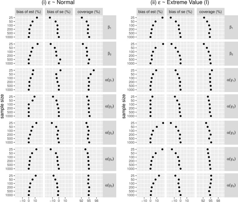
The performance of CPMs on estimating the slopes β₁, β₂, and α(y) at y₁ = e⁻¹ ≈ 0.368, y₂ = e^−0.33 ≈ 0.719, y₃ = e^0.5 ≈ 1.649, y₄ = e^1.33 ≈ 3.781, and y₅ = e² ≈ 7.389 with properly specified link functions: (i) ε ~ Normal and (ii) ε ~ Extreme Value (I).

We also investigated the relative efficiency of the properly specified CPMs compared with other commonly used parametric or semiparametric models. For error distribution (i), we compared the CPM with the linear regression model after a Box-Cox transformation [20]:

$$B(y;\mathrm{\lambda })=\{\begin{array}{ll}(y^{\mathrm{\lambda }}-1)/\mathrm{\lambda }\hfill & \text{if}\mathrm{\lambda }\ne 0;\hfill \\ \log (y)\hfill & \text{if}\mathrm{\lambda }=0.\hfill \end{array}$$

The usual practice of Box-Cox transformation is to first find the $\widehat{\mathrm{\lambda }}$ which gives the highest profile likelihood for the transformed linear regression model, and then to treat $\widehat{\mathrm{\lambda }}$ as known (which is potentially problematic because it ignores uncertainty in its estimation) and transform the response y to $y^{\ast }=B(y;\widehat{\mathrm{\lambda }})$, and finally, to fit linear regression with y^∗ as the outcome. In our simulations, we performed the Box-Cox transformation using the boxcox() function in the MASS R package [21]. We used its default option in which λ is estimated by a grid search algorithm searching in the range of −2 to 2 with increments of 0.1.

In our simulation setting, the proper transformation, log(y), is a special case of the Box-Cox transformation with parameter λ = 0. With the latent scale error ε ~ N(0, 1), the Box-Cox transformation model is a properly specified parametric transformation model. Figure 7 (i) shows the relative efficiency of the properly specified CPM compared with the Box-Cox transformation model on estimating the slopes β₁ and β₂. Since the estimates from the CPM show small bias when the sample size is small, we estimate the relative efficiency with the ratio of mean squared errors (MSE) instead of the ratio of variances. As expected, the properly specified CPM is generally less efficient than its parametric counterpart. However, the relative efficiency increases with the sample size. Specifically, in our simulation setting, the relative efficiency is over 80% when n = 100, and over 90% when n = 1, 000, indicating only a small efficiency loss when using properly specified CPMs with moderate or large sample sizes.

Figure 7.

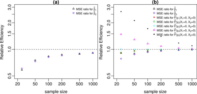
(i): The relative efficiency of properly specified CPM (using the probit link function) compared with properly specified Box-Cox transformation model; (ii): The relative efficiency of properly specified CPM (using the cloglog link function) compared with Cox proportional hazard model.

For error distribution (ii), we compared the properly specified CPM with the Cox proportional hazards model. In this scenario, both models assume proportional hazards and are properly specified semiparametric models. However, their estimation procedures are different. The Cox proportional hazards model maximizes the partial likelihood which is only a function of slopes, whereas the CPM maximizes the full likelihood L^∗ which is a function of both intercepts and slopes. The intercepts (i.e., baseline log-cumulative hazard) of the Cox model can be estimated post hoc with the Breslow estimator [22], from which one can compute the cumulative probabilities. Usually, the Cox proportional hazards model is applied to right censored data, but it can also be fitted to uncensored data with negative values. Figure 7 (ii) shows the relative efficiency (again, measured with MSE ratio) of the CPM and Cox proportional hazards model on estimating β₁ and β₂, and baseline cumulative probabilities (i.e., X₁ = X₂ = 0) at y₁,…, y₅. In our simulations, the CPM with the cloglog link function has similar performance with the Cox proportional hazards model when the sample size is moderate or large. With smaller sample sizes, however, the CPM is generally less efficient for estimating the slopes, but more efficient for estimating the cumulative probabilities.

As described in Section 2.2, the conditional CDF and other properties of the conditional distribution can be derived with the regression coefficients from CPMs. Figure 8 summarizes the performance for estimating conditional CDFs when the link function is properly specified. The performance of CPMs for estimating conditional means and conditional quantiles are summarized in Supplemental Materials Figure S.1 and Figure S.2, respectively. Similar patterns are observed as in estimating the regression coefficients. Generally, the CPMs have good performance for estimating different aspects of the conditional distribution with moderate or large sample sizes (e.g., n ≥ 50 in our simulation settings). But when the sample size is relatively small (e.g., n = 25), there may be substantial bias both in estimating the parameters and their standard errors. Presumably this is because the NPMLE approximation is more accurate with bigger sample sizes.

Figure 8.

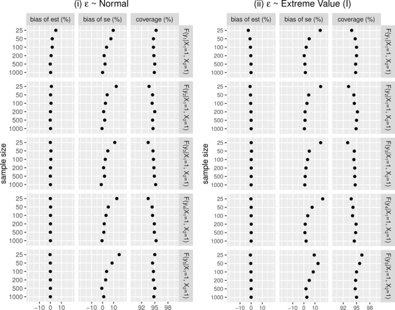
The performance of CPMs on estimating conditional CDF given X₁ = 1 and X₂ = 1, evaluated at y₁ = 0.368, y₂ = 0.719, y₃ = 1.649, y₄ = 3.781, and y₅ = 7.389 with properly specified link functions: (i) ε ~ Normal and (ii) ε ~ Extreme Value (I). The results are based on 10,000 simulation replicates for each sample size.

Although the CPM is usually less efficient than the properly specified parametric models, it may still have some advantage when estimating some properties that are easier to derive from the conditional CDF. For example, with the error distribution (i) where the Box-Cox transformation model is properly specified, although the CPM is generally less efficient for estimating the slope parameters, it has good performance for estimating the conditional mean with moderate to large sample sizes when the link function is properly specified. However, for the Box-Cox transformation model, we often only consistently estimate the conditional mean on the transformed scale, i.e., Ŷ ∗ → E[B(Y, λ)|X]. Performing a simple back transformation, $B^{-1}({\widehat{Y}}^{\ast },\widehat{\mathrm{\lambda }})$, usually does not yield a consistent estimator for the conditional mean on the original scale because $B^{-1}({\widehat{Y}}^{\ast },\widehat{\mathrm{\lambda }})\to B^{-1}\{E[B(Y,\mathrm{\lambda })|X],\mathrm{\lambda }\}$, which is well known from Jensen’s inequality to not equal E(Y|X) except when λ = 1.

3.2. Estimation with Link Function Misspecification

Although the commonly used link functions represent various types of error distributions, e.g., the probit and logit link functions correspond to bell-shaped and symmetric error distributions with different tail densities, whereas cloglog and loglog link functions represent error distributions skewed in opposite directions, in practice there is no guarantee that the latent error has exactly the same CDF as the inverse of the link function. Therefore, it is of interest to study the robustness of CPMs with link function misspecification, especially when the misspecification is only moderate, e.g., using the probit link function when the true latent error distribution is the t-distribution or using the cloglog/loglog link functions when the true error distribution is skewed in the same direction but does not have exactly the same shape as the specified link function. We generated data from Y = H(β₁X₁ + β₂X₂ + ε), where X₁ ~ Bernoulli(0.5), X₂ ~ N(0, 1), β₁ = 1 and β₂ = −0.5. For simplicity, we set H(y) = y, that is, no transformation is needed. The error term ε is generated from: (a) the standard normal distribution, (b) the standard logistic distribution, (c) the Type I extreme value distribution, (d) the Type II extreme value distribution, (e) t₅, the t distribution with 5 degrees of freedom, (f) the uniform distribution with range from −5 to 5, (g) the standardized beta distribution with parameters α = 5 and β = 2 (standardized by subtracting the mean and then dividing by the standard deviation), and (h) the standardized beta distribution with parameters α = 2 and β = 5. The probability density functions (PDFs) of these error distributions and the extent of violation to the parallelism assumption with probit, logit, cloglog, and loglog link functions are shown in Supplemental Materials S.2.2 (see Figures S.3 and S.4). The proper link functions for (a) – (d) are probit, logit, cloglog, and loglog, respectively, whereas, there are no proper link functions with existing software for (e) – (h), i.e., no perfect parallelism.

We fitted CPMs with probit, logit, cloglog, and loglog link functions for each scenario with sample sizes of 50, 100, and 200, respectively. With different link functions, the regression coefficients are not in the same scale, and therefore are not directly comparable. Instead, we compared the estimated conditional means and conditional medians for (X₁ = 0, X₂ = 0), (X₁ = 1, X₂ = 0), (X₁ = 0, X₂ = 1), and (X₁ = 1, X₂ = 1). For the purpose of comparison, we also obtained the estimates for these conditional means and medians from linear regression and median regression models. The efficiency of the CPM on estimating conditional means and medians is compared with the properly specified linear regression and median regression models, respectively.

Figures 9 and 10 summarize the performance for estimating conditional means and medians, respectively, for sample sizes of 100. More details of these simulation results, as well as those for sample sizes of 50 and 200 (which yielded similar results), are reported in Supplemental Materials S.2.2. In summary, we find with moderate or large sample size (e.g., n ≥ 50), the CPMs with properly specified link functions have good performance for estimating conditional means and medians, i.e., the bias is small and the coverage probability of 95% confidence intervals is close to 0.95. It is worth pointing out that CPMs with properly specified link functions seem to be more efficient than median regression, i.e., MSE ratios are generally greater than 1. CPMs with properly specified link functions may also be more efficient than linear regression when the error distribution is skewed, e.g., error distribution (c) (Type I extreme Value) with the cloglog link function and error distribution (d) (Type II extreme value) with the loglog link function. The CPMs seem to have reasonable performance under minor or moderate link function misspecification, e.g., error distribution (a) (Normal) with the logit link function, (b) (Logistic) with the probit link function, (e) (t₅) with the logit or probit link function, (g) (standardized Beta(5, 2)) with the cloglog link function, and (h) (standardized Beta(2, 5)) with the loglog link function. However, with severe link function misspecification, i.e., the error distributions have totally different shapes or are skewed in opposite directions, the CPMs may have poor performance, e.g., error distributions (a) (Normal) and (b) (Logistic) with the cloglog or loglog link functions, error distributions (c) (Type I extreme value) and (g) (standardized Beta(5, 2)) with the loglog link function, and error distributions (d) (Type II extreme value) and (h) (standardized Beta(2, 5)) with the cloglog link function.

Figure 9.

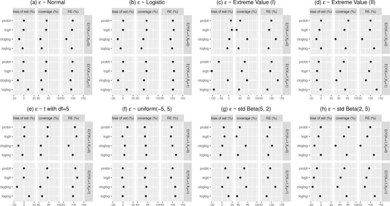
The performance of CPMs on estimating conditional means with commonly used link functions. We summarize the percent bias (%) of the point estimate, the coverage probability of 95% confidence intervals, and the relative efficiency (RE) for (X₁ = 1, X₂ = 0) and (X₁ = 1, X₂ = 1) with sample size of 100 in this plot. The percent bias of the point estimate is calculated as the mean of point estimates in 10,000 simulation replicates minus the true value and then divided by the true value. The RE is compared with properly specified linear regression measured with MSE ratio. Numerical summary of these results are provided in Supplemental Materials S.2.2.

Figure 10.

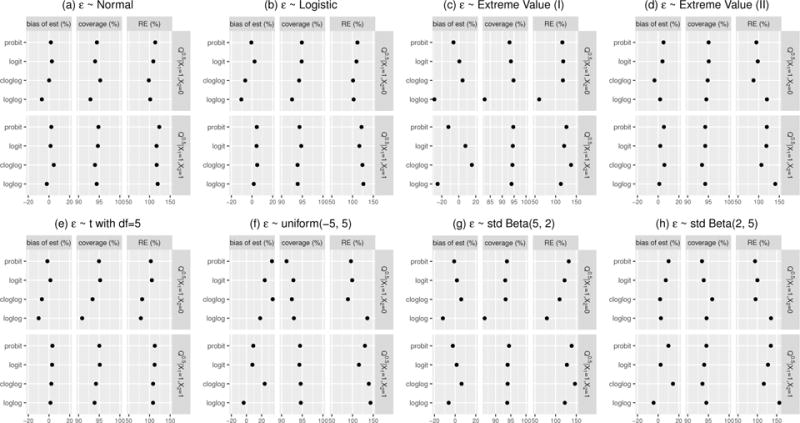
The performance of CPMs on estimating medians with commonly used link functions. The description is similar as that for Figure 9 except that the RE is compared with properly specified median regression.

As one of the reviewers suggested, we also conducted simulations to explore the performance of CPMs with more extreme covariate distributions, with the inclusion of an interaction term between X₁ and X₂, and with different choices of β. The results were generally similar with those already reported, except that larger sample sizes were needed to obtain stable and unbiased estimates in these more complicated settings. Details of these simulation results can be found in Supplemental Materials S.2.3.

3.3. Computation Time

Because estimation requires inverting a Hessian matrix whose dimensions increase with the sample size, computation time of CPMs with continuous outcomes substantially increases with n, even when taking advantage of the block tridiagonal nature of the Hessian (see Section 2.2). For example, generating data as described in Section 3.1 with normal errors, the average computation times based on 100 replications with the properly specified model using the orm () function in R software were 1.3, 21, 82, and 338 seconds for sample sizes of 1000, 5000, 10000, and 20000, respectively. (These and all other simulations in this subsection were performed using a 2012 iMac with 3.4 GHz Intel Core i7 and 16 GB 1600 MHz DDR3.) In contrast, properly transforming the data and then fitting a linear model took an average of 0.013 seconds for n = 20000.

Computation time decreases as the number of unique outcomes decreases. We repeated the simulation described above, but reduced the number of unique outcomes by binning the continuous response variables evenly into a large number of bins, varying from 100 to 10000, based on quantiles of the simulated data. Figure 11 shows the length of time for estimation in these simulations as a function of the number of unique outcomes. For example, with n = 20000, average computation time went from 338 seconds with no binning to 1.2 seconds binning to 100 outcomes. Estimates using the binned data tended to be similar to those without binning, even when binning to as few as 100 unique categories, with bias remaining about the same and only minor increases in the MSE for most parameters (see Tables S.23 and S.24 in Supplemental Materials). After binning, we were able to fit cumulative probability models to data with very large n; with n = 10 million and binning to 200 unique outcomes based on quantiles, model fitting took approximately 25 minutes.

Figure 11.

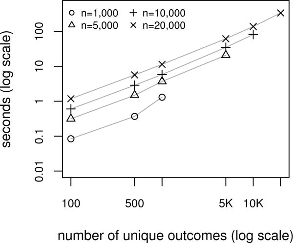
Average time to fit the cumulative probability model versus the average number of unique outcomes for different sample sizes, n. Results are based on 100 replications.

It should be noted that in practice continuous data are usually obtained in rounded forms. For example, time is often recorded in days, body-mass index rounded to one decimal, and so forth. Hence, in practice the number of unique outcomes typically does not equal the sample size as n gets very large, even with unbounded data. However, if data are truly continuous, these results suggest that with very large n, an analyst might consider binning the outcomes prior to fitting CPMs with little sacrifice in accuracy of estimation.

4. Application Examples

We illustrate the application of CPMs for continuous outcomes using a dataset of 4,776 persons living with HIV starting antiretroviral therapy (ART) in Latin America [23]. CD4 count and viral load are important measures of an HIV-positive patient’s immune system function and control of the virus. We are interested in modeling CD4 count and viral load 6 months after the initiation of ART using patients’ demographics and baseline covariates, summarized in Supplemental Materials Table S.25. Both variables’ distributions are typically skewed. When modeling them with linear regression models, transformations are often applied, e.g., square root transformation for CD4 count and log transformation for viral load, although other transformations are sometimes used and different transformations may yield conflicting results. With CPMs, the proper transformation can be estimated semiparametrically or ignored. In addition, measurements of viral load are often censored at assay detection limits, especially when patients are on ART. To deal with this issue, common practice is to categorize the viral load (e.g., “undetectable” versus “detectable”) or to impute particular values for those measurements below the detection limit (e.g., if the detection limit is 400 copies/mL, then to record all measurements below the detection limit as 399 copies/mL). However, these strategies either ignore the information of viral load above the detection limit or make assumptions for viral load below the detection limit. We believe that CPMs are particularly useful in these settings.

4.1. CD4 Count

We fit CPMs for CD4 count 6 months after ART initiation with the probit, logit, cloglog, and loglog link functions, including age, gender, treatment class, study site, probable infection route, year of ART initiation, baseline nadir CD4, baseline viral load, and baseline AIDS status as covariates. These CPMs have a total of 831 intercepts for 832 unique CD4 values. The baseline nadir CD4 was square-root transformed, and then modeled with restricted cubic splines using 5 knots. The baseline viral load was log transformed, and then modeled with restricted cubic splines using 5 knots. All other continuous predictors were transformed with restricted cubic splines using 5 knots directly. The CPM with the loglog link function did not converge after 12 iterations, suggesting poor model fit, and was not considered further.

Figure 12 (a) plots the estimated intercepts â(y) resulting from the CPMs, which can be interpreted as semiparametric estimates of the best transformation for the 6-month CD4 count. For purpose of comparison, we also plot the estimated Box-Cox transformation, which was estimated to be (y^0.421 − 1)/0.421, close to the commonly used square-root transformation.

Figure 12.

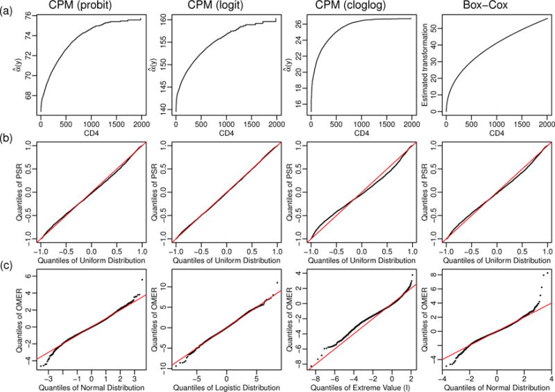
(a): the estimated intercepts â(y) from the CPMs using the probit, logit, and cloglog link functions, which can be interpreted as semiparametric estimates of the best transformation for the 6-month CD4 count. For purpose of comparison, we also plot the estimated Box-Cox transformation, (b): QQ-plots of probability-scale residuals (PSRs). (c): QQ-plots of observed-minus-expected residuals (OMERs), removing the residual for the observation with the largest value of 6-month CD4 count.

The log likelihoods for models using the probit, logit, and cloglog link functions were −28796.59, −28709.87, and −29185.60, respectively, suggesting better model fit using the symmetric probit and logit link functions. To further assess the goodness-of-fit with different link functions, we computed the probability-scale residuals (PSRs), defined as P (Y^* < y) − P (Y^* > y), where y is the observed value and Y^* is a random variable from the fitted distribution [18, 19]. PSRs of a continuous outcome under the properly specified model are approximately uniformly distributed with range from −1 to 1. Therefore, the QQ-plot of PSRs versus the uniform distribution can be used to assess the overall model fit (Figure 12 (b)). We can also assess the model fit using the observed-minus-expected residuals (OMERs) on the transformed scale. Specifically, since the CPM (3) can be interpreted as the semiparametric transformation model Y = H(βX + ε) and the intercept α(y) = H⁻¹(y), we can compute the OMERs on the transformed scale as ${\widehat{\epsilon }}_i=\widehat{\alpha }(y_i)-\widehat{\beta }{x}_i$. However, as discussed in Section 2.2, the NPMLE of α(y) is an unbounded step function with â(y_max) = +∞; therefore, the OMER for the observation with the largest value of y is also unbounded. Figure 12 (c) shows the QQ plot of OMERs versus the error distributions corresponding to the specific link functions, removing the residual for the observation with the largest CD4 count. Both (b) and (c) of Figure 12 suggest better model fit using the logit link function. This is consistent with the fact that the CPM with the logit link function has the highest log likelihood among all link functions considered. The QQ-plots of PSRs and OMERs from the linear regression model with Box-Cox transformation are also shown in Figure 12, suggesting after the Box-Cox transformation, the error distribution, although fairly symmetric, is not normally distributed, especially in the tail regions.

PSRs and OMERs can also be used in residual-by-predictor plots to detect the lack of fit for models. For example, in Figure 13, we compare the residual-by-predictor plots using both PSRs and OMERs from the CPMs including and not including the baseline nadir CD4 in the model. The smoothed curves show a clear pattern of a positive relationship between residuals and the baseline nadir CD4 when it is not included (left panel of Figure 13). The relationship disappears when the baseline nadir CD4 is included (right panel of Figure 13).

Figure 13.

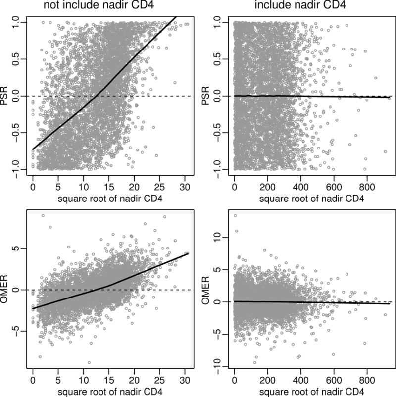
Residual-by-predictor plots using probability-scale residuals (PSRs) (top panel) and observed-minus-expected residuals (OMERs) on the transformed scale (bottom panel) from CPMs (using the logit link function) including and not including baseline nadir CD4 count in the models. Smoothed curves using Friedman’s super smoother are added.

As described in Section 2.2, one can easily obtain different aspects of conditional distributions using CPMs for continuous outcomes. This is particularly useful when modeling CD4 count. For example, we might want to summarize the central tendency of the conditional distribution with medians instead of means since the distribution is skewed. Besides the central tendency, we may also be interested in the probabilities of CD4 count below or above some commonly used thresholds. Figure 14 plots the estimated means, medians, and the probabilities of CD4 count being above 350 or 500 cells/μL as functions of age or treatment class fixing other predictors at their medians (for continuous variables) or modes (for categorical variables). For purpose of comparison, we also obtained the conditional means through a back transformation from the linear regression model with the Box-Cox transformation, the conditional medians from a median regression model, and the conditional probabilities of CD4 being above 350 or 500 cells/μL from corresponding binary logistic regression models using dichotomized CD4 count as outcomes. All models included the same predictor variables (and their transformations).

Figure 14.

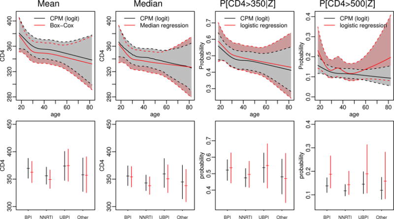
The estimated mean, median, and the probabilities of CD4 being greater than 350 cells/μL and CD4 being greater than 500 cells/μL as functions of age (top panel) or treatment class (bottom panel, BPI: boosted protease inhibitors, NNRTI: non-nucleoside reverse transcriptase inhibitors, and UBPI: unboosted protease inhibitors) from the CPM with the logit link function fixing other predictors at their medians (for continuous variables) or modes (for categorical variables). For purpose of comparison, we also plot the conditional means from linear regression models with Box-Cox transformation, the conditional medians from median regression models, and conditional probabilities from logistic regression models using the dichotomized CD4 count as outcomes. The shaded regions are point-wise 95% confidence intervals.

The estimated conditional means and medians from the different models were generally similar with comparable 95% confidence intervals except that some point estimates for conditional means from the back transformation of linear models were slightly lower than those from the CPM. This trend is generally consistent with the direction of Jensen’s inequality, i.e., E[g(Y|X)] ≤ g[E(Y|X)], where g(y) = (y^0.421 − 1)/0.421. The CPMs were more efficient at estimating the conditional probabilities of CD4 count being above 350 or 500 cells/μL than the corresponding logistic regression models as evidenced by their narrow 95% confidence intervals. It is interesting to note that the two models give similar point estimates for the probabilities of CD4 count being above 350 cells/μL but slightly different point estimates for the probabilities of CD4 count being above 500 cells/μL. The estimates from the logistic regression models tend to be larger, presumably due to the loss of information resulting from grouping the outcome into two categories.

In summary, rather than fitting three separate models, some of which require transforming the outcome, we were able to obtain similar and likely less biased and more efficient estimates by fitting a single CPM.

4.2. Viral Load

In this dataset, 85.5% of the patients had viral load (VL) below the detection limit (400 copies/mL) 6 months after ART initiation. For those measurements above the detection limit, their distribution was highly skewed, ranging from 400 to 7,800,000 copies/mL with a median of 1,300 copies/mL. Due to the large proportion of undetectable viral loads, common practice is to dichotomize the viral load into two categories (“undetectable” and “detectable”) and then fit logistic regression models, which ignores the numerical information in the detectable measurements. To make full use of ordinal information of viral load, we fit CPMs for the 6-month viral load measures using the probit, logit, cloglog, and loglog link functions. These CPMs have a total of 443 intercepts for 444 unique viral values. We included the same covariates with similar transformations as in the CD4 models except that we used 4 knots when transforming the continuous variables using restricted cubic splines because of concerns of over-fitting due to the large proportion of undetectable viral loads.

The log likelihoods for models using the probit, logit, cloglog, and loglog link functions were −5213.69, −5185.26, −5245.03, and −5162.70, respectively, suggesting better model fit with the skewed loglog link function, followed by the symmetric logit and probit link functions, then the cloglog link function which is skewed in the opposite direction as the loglog link function. The estimated transformations and the QQ-plots of PSRs and OMERs are provided in Figure S.8 and Figure S.9 in Supplemental Materials S.3. Note, since the distribution of 6-month viral load is a mixture of discrete and continuous distributions, PSRs are not uniformly distributed, even if the model is properly specified. OMERs on the transformed scale similarly suffer. Therefore QQ-plots, in this setting, are not useful for assessing model fit. In this example, although the model with the loglog link function had a slightly higher log likelihood, we also consider the logit probability model for purpose of convenient interpretation, particularly for comparisons with logistic regression models on the dichotomized viral load outcome. Although PSRs are generally not uniformly distributed for variables with mixed types of discrete and continuous distributions, they have expectation 0 under properly specified models, and therefore can still be used in residual-by-predictor plots [19], as is shown in Figure S.9 in Supplemental Materials S.3. The results using the loglog and the logit link functions are generally similar.

Figure 15 plots the estimated probabilities of 6-month viral load being detectable and being greater than 1,000 copies/mL as functions of age or treatment class fixing other predictors at their medians or modes using both the loglog and the logit link functions. The results using these two different link functions were very similar. For purpose of comparison, we also obtained the estimated probabilities from logistic regression models using dichotomized viral loads as the outcomes (VL detectable vs non-detectable, and VL>1,000 copies/mL vs VL ≤ 1,000 copies/mL). CPMs and logistic regression models gave very similar results when estimating the probabilities of 6-month viral load being detectable: similar point estimates and comparable 95% confidence intervals. Results were more different when estimating the probabilities of 6-month viral load being greater than 1,000 copies/mL: the point estimates from the CPMs were generally smaller with narrower 95% confidence intervals than those from logistic regression models, as the CPMs incorporated information from all levels of detectable viral loads.

Figure 15.

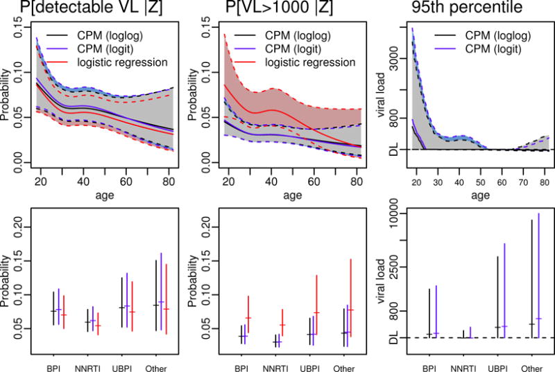
The probabilities of 6-month viral load (VL) being detectable (≥ 400 copies/mL) and being greater than 1000 copies/mL, and the 95^th percentiles as functions of age (top panel) or treatment class (bottom panel), estimated using the CPM with the loglog and logit link functions, fixing other predictors at their medians (for continuous variables) or modes (for categorical variables). The shaded regions are the point-wise 95% confidence intervals. For purpose of comparison, we also show the estimates of the conditional probabilities from logistic regression models using the dichotomized viral load as the outcome. We also estimated conditional percentiles from quantile regression models by imputing the measurements below the detection limit to be the detection limit or 0. However, since the estimates from quantile regression models were very unstable with very wide 95% confidence intervals crossing 0, we did not plot the results.

Figure 15 also contains the estimated 95^th percentiles using the two link functions. We also seeked to obtain estimates of the 95^th percentiles from two separate quantile regression models: one imputing values below the detection limit as the detection limit (i.e., 400 copies/mL) and the other imputing values below the detection limit as 0. The estimates from the quantile regression models were very unstable: the point estimates varied with values imputed for undetectable viral load and their 95% confidence intervals were very wide (with negative values for the lower bounds, results not shown). In contrast, CPMs did not require any imputation and they gave sensible point estimates and 95% confidence intervals.

We performed a limited simulation to compare the performance of CPMs, logistic regression models with dichotomized outcomes, and linear regression models with imputed values under various undetectable proportions (see Table S.26 in Supplemental Materials S.4). We found that CPMs with properly specified link functions were generally more efficient than the other two approaches. We also saw that gains in efficiency, particularly when compared with logistic regression models, were minimal when the proportion of undetectable measurements was large, e.g. ≥ 75%, as was the case in our actual data example.

5. Discussion

In this paper, we have studied CPMs for continuous outcomes. By relating them to semiparametric transformation models, we have shown that the intercepts from CPMs can be viewed as the estimated semiparametric transformation. Therefore, fitting ordinal regression models to continuous data can completely bypass the issue of guessing the proper transformation for response variables, which makes these models particularly useful when flexible transformations are needed. Another suitable application of these models is for measurements with detection limits, since they only require outcomes to be orderable, but do not require assigning specific values to those under the detection limit. Various aspects of the conditional distribution can be easily derived from the regression coefficients, giving a full picture of the conditional distribution. Of course, the flexibility and robustness of CPMs comes with costs in terms of statistical and computational efficiency. However, our simulations suggest that for moderate sample sizes the relative efficiency of CPMs versus properly specified parametric models is not bad, and although computation time is slower than traditional regression analyses, fitting CPMs with large n is feasible.

Manuguerra and Heller [24] also advocated fitting a type of ordinal regression model to continuous data, specifically data from visual analog scales. Rather than nonparametrically estimating the intercepts in CPMs, their approach fits a smooth curve to the intercepts, either using a parametric model or B-splines. Hence, their approach is likely more efficient but less robust than that considered in this manuscript. Their approach is also more difficult to implement as it differs from traditional CPMs typically used for the analysis of ordinal data. With that said, the premise of their method is promising, and certainly warrants consideration and further study.

Our simulation studies show that properly specified CPMs have good finite sample performance with moderate or relatively large sample sizes, but that some bias may occur when the sample size is small. In addition, CPMs seem to be fairly robust to minor or moderate link function misspecification. These results are comforting given that the asymptotic properties of the NPMLE of these models have not been formally developed and are quite challenging ([12]; personal communication with Zeng, Kosorok, & Lin). We have focused on the application side of these models and we hope our study provides additional motivation and insight to this challenging theoretical problem.

Using CPMs for continuous variables is motivated from a simple and intuitive idea: continuous variables are also ordinal and can be modeled ordinally. This idea can be naturally extended to other ordinal regression models, such as the continuation-ratio model and the adjacent-categories model, and to more complicated settings, such as longitudinal data in which the observations are not independent. We are studying extensions in these settings.

References

- 1.Sall J. A monotone regression smoother based on ordinal cumulative logistic regression. ASA Proceedings of Statistical Computing Section. 1991:276–281. [Google Scholar]
- 2.Harrell FE. Regression Modeling Strategies: With Applications to Linear Models, Logistic and Ordinal Regression, and Survival Analysis. Second. Springer; 2015. [Google Scholar]
- 3.Walker SH, Duncan DB. Estimation of the probability of an event as a function of several independent variables. Biometrika. 1967;54(1–2):167–179. [PubMed] [Google Scholar]
- 4.McCullagh P. Regression models for ordinal data. Journal of the Royal Statistical Society Series B (Methodological) 1980;42(2):109–142. [Google Scholar]
- 5.Fienberg SE. The Analysis of Cross-classified Categorical Data. Second. MIT Press; Cambridge, MA: 1980. (reprinted by Springer, New York, 2007) [Google Scholar]
- 6.Tutz G. Sequential item response models with an ordered response. British Journal of Mathematical and Statistical Psychology. 1990;43(1):39–55. [Google Scholar]
- 7.Simon G. Alternative analyses for the singly-ordered contingency table. Journal of the American Statistical Association. 1974;69(348):971–976. [Google Scholar]
- 8.Goodman LA. The analysis of dependence in cross-classifications having ordered categories, using log-linear models for frequencies and log-linear models for odds. Biometrics. 1983;39(1):149–160. [PubMed] [Google Scholar]
- 9.Anderson JA. Regression and ordered categorical variables. Journal of the Royal Statistical Society Series B (Methodological) 1984;46(1):1–30. [Google Scholar]
- 10.Agresti A. Analysis of Ordinal Categorical Data. Second. John Wiley & Sons; 2010. pp. 118–130. [Google Scholar]
- 11.Harrell FE. rms: Regression Modeling Strategies. 2016 URL http://CRAN.R-project.org/package=rms, R package version 4.5-0.
- 12.Zeng D, Lin D. Maximum likelihood estimation in semiparametric regression models with censored data. Journal of the Royal Statistical Society Series B (Methodological) 2007;69(4):507–564. [Google Scholar]
- 13.R Core Team. R: A Language and Environment for Statistical Computing. R Foundation for Statistical Computing; Vienna, Austria: p. 2016. URL https://www.R-project.org/ [Google Scholar]
- 14.Casella G, Berger RL. Statistical Inference. Second. Cengage Learning; 2002. [Google Scholar]
- 15.Genter FC, Farewell VT. Goodness-of-link testing in ordinal regression models. Canadian Journal of Statistics. 1985;13(1):37–44. [Google Scholar]
- 16.Huberty CJ. Problems with stepwise methods – better alternatives. Advances in Social Science Methodology. 1989;1:43–70. [Google Scholar]
- 17.Shepherd BE. The cost of checking proportional hazards. Statistics in Medicine. 2008;27(8):1248–1260. doi: 10.1002/sim.3020. [DOI] [PubMed] [Google Scholar]
- 18.Li C, Shepherd BE. A new residual for ordinal outcomes. Biometrika. 2012;99(2):473–480. doi: 10.1093/biomet/asr073. [DOI] [PMC free article] [PubMed] [Google Scholar]
- 19.Shepherd BE, Li C, Liu Q. Probability-scale residuals for continuous, discrete, and censored data. Canadian Journal of Statistics. 2016;44(4):463–479. doi: 10.1002/cjs.11302. [DOI] [PMC free article] [PubMed] [Google Scholar]
- 20.Box GEP, Cox DR. An analysis of transformations. Journal of the Royal Statistical Society Series B (Methodological) 1964;26(2):211–252. [Google Scholar]
- 21.Venables WN, Ripley BD. Modern Applied Statistics with S. Fourth. Springer; New York: 2002. URL http://www.stats.ox.ac.uk/pub/MASS4. [Google Scholar]
- 22.Breslow NE. Discussion of Professor Cox’s paper. J Royal Stat Soc B. 1972;34:216–217. [Google Scholar]
- 23.McGowan CC, Cahn P, Gotuzzo E, Padgett D, Pape JW, Wolff M, Schechter M, Masys DR. Cohort Profile: Caribbean, Central and South American Network for HIV research (CCASAnet) collaboration within the International Epidemiologic Databases to Evaluate AIDS (IeDEA) programme. International Journal of Epidemiology. 2007;36(5):969–976. doi: 10.1093/ije/dym073. [DOI] [PubMed] [Google Scholar]
- 24.Manuguerra M, Heller GZ. Ordinal regression models for continuous scales. The International Journal of Biostatistics. 2010;6(1) doi: 10.2202/1557-4679.1230. [DOI] [PubMed] [Google Scholar]
Associated Data
This section collects any data citations, data availability statements, or supplementary materials included in this article.