Significance
Humans have difficulty seeing small motions with amplitudes below a threshold. Although there are optical techniques to visualize small static physical features (e.g., microscopes), visualization of small dynamic motions is extremely difficult. Here, we introduce a visualization tool, the motion microscope, that makes it possible to see and understand important biological and physical modes of motion. The motion microscope amplifies motions in a captured video sequence by rerendering small motions to make them large enough to see and quantifies those motions for analysis. Amplification of these tiny motions involves careful noise analysis to avoid the amplification of spurious signals. In the representative examples presented in this study, the visualizations reveal important motions that are invisible to the naked eye.
Keywords: visualization, motion, image processing
Abstract
Although the human visual system is remarkable at perceiving and interpreting motions, it has limited sensitivity, and we cannot see motions that are smaller than some threshold. Although difficult to visualize, tiny motions below this threshold are important and can reveal physical mechanisms, or be precursors to large motions in the case of mechanical failure. Here, we present a “motion microscope,” a computational tool that quantifies tiny motions in videos and then visualizes them by producing a new video in which the motions are made large enough to see. Three scientific visualizations are shown, spanning macroscopic to nanoscopic length scales. They are the resonant vibrations of a bridge demonstrating simultaneous spatial and temporal modal analysis, micrometer vibrations of a metamaterial demonstrating wave propagation through an elastic matrix with embedded resonating units, and nanometer motions of an extracellular tissue found in the inner ear demonstrating a mechanism of frequency separation in hearing. In these instances, the motion microscope uncovers hidden dynamics over a variety of length scales, leading to the discovery of previously unknown phenomena.
Motion microscopy is a computational technique to visualize and analyze meaningful but small motions. The motion microscope enables the inspection of tiny motions as optical microscopy enables the inspection of tiny forms. We demonstrate its utility in three disparate problems from biology and engineering: visualizing motions used in mammalian hearing, showing vibration modes of structures, and verifying the effectiveness of designed metamaterials.
The motion microscope is based on video magnification (1–4), which processes videos to amplify small motions of any kind in a specified temporal frequency band. We extend the visualization produced by video magnification to scientific and engineering analysis. In addition to visualizing tiny motions, we quantify both the object’s subpixel motions and the errors introduced by camera sensor noise (5). Thus, the user can see the magnified motions and obtain their values, with variances, allowing for both qualitative and quantitative analyses.
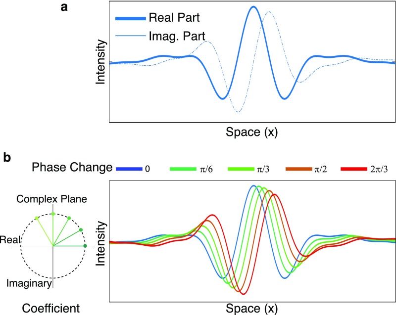
The motion microscope characterizes and amplifies tiny local displacements in a video by using spatial local phase. It does this by transforming the captured intensities of each frame’s pixels into a wavelet-like representation where displacements are represented by phase shifts of windowed complex sine waves. The representation is the complex steerable pyramid (6), an overcomplete linear wavelet transform, similar to a spatially localized Fourier transform. The transformed image is a sum of basis functions, approximated by windowed sinusoids (Fig. S1), that are simultaneously localized in spatial location (), scale , and orientation . Each basis function coefficient gives spatially local frequency information and has an amplitude and a phase .
Fig. S1.
Increasing the phase of complex steerable pyramid coefficients results in approximate local motion of the basis functions. (A) A 1D slice of a complex steerable pyramid basis function. (B) The basis function is multiplied by several complex coefficients of constant amplitude and increasing phase to produce the real part of a new basis function that is approximately translating. Copyright (2016) Association for Computing Machinery, Inc. Reprinted with permission from ref. 37.
To amplify motions, we compute the unwrapped phase difference of each coefficient of the transformed image at time from its corresponding value in the first frame,
| [1] |
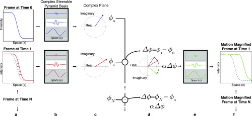
We isolate motions of interest and remove components due to noise by temporally and spatially filtering . We amplify the filtered phase shifts by the desired motion magnification factor to obtain modified phases for each basis function at each time . We then transform back each frame’s steerable pyramid to produce the motion-magnified output video (Fig. S2) (3).
Fig. S2.
A 1D example illustrating how the local phase of complex steerable pyramid coefficients is used to amplify the motion of a subtly translating step edge. (A) Frames (two shown) from the video. (B) Sample basis functions of the complex steerable pyramid. (C) Coefficients (one shown per frame) of the frames in the complex steerable pyramid representation. The phases of the resulting complex coefficients are computed. (D) The phase differences between corresponding coefficients are amplified. Only a coefficient corresponding to a single location and scale is shown; this processing is done to all coefficients. (E) The new coefficients are used to shift the basis functions. (F) A reconstructed video is produced by inverse transforming the complex steerable pyramid representation. The motion of the step edge is magnified. Copyright (2016) Association for Computing Machinery, Inc. Reprinted with permission from ref. 37.
We estimate motions under the assumption that there is a single, small motion at each spatial location. In this case, each coefficient’s phase difference, , is approximately equal to the dot product of the corresponding basis function’s orientation and the 2D motion (7) (Relation Between Local Phase Differences and Motions). The reliability of spatial local phase varies across scale and orientations, in direct proportion to the coefficient’s amplitude (e.g., coefficients for basis functions orthogonal to an edge are more reliable than those along it) (Fig. S3 and Low-Amplitude Coefficients Have Noisy Phase). We combine information about the motion from multiple orientations by solving a weighted least squares problem with weights equal to the amplitude squared. The result is a 2D motion field. This processing is accurate, and we provide comparisons to other algorithms and sensors (Fig. 1, Synthetic Validation, and Figs. S4 and S5).
Fig. S3.
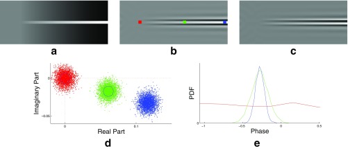
Noise model of local phase. (A) A frame from a synthetic video with noise. (B) The real part of a single level of the complex steerable pyramid representation of A. (C) The imaginary part of the same level of the complex steerable pyramid representation of A. (D) A point cloud over noisy values of the real and imaginary values of the complex steerable pyramid representation at the red, green, and blue points in B. (E) The corresponding histogram of phases.
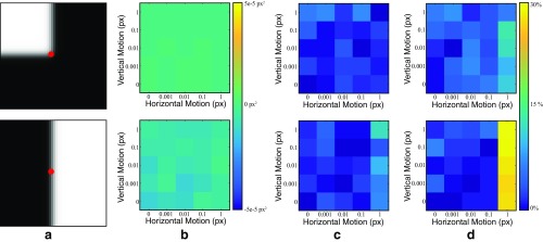
Fig. 1.
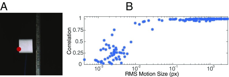
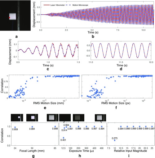
A comparison of our quantitative motion estimation vs. a laser vibrometer. Several videos of a cantilevered beam excited by a shaker were taken with varying focal length, exposure times, and excitation magnitude. The horizontal, lateral motion of the red point was also measured with a laser vibrometer. (A) A frame from one video. (B) The correlation between the two signals across the videos vs. root mean square (RMS) motion size in pixels (px). Only motions at the red point in A were used in our analysis. More results are in Fig. S4.
Fig. S4.
A comparison of our quantitative motion estimation vs. a laser vibrometer. Several videos of a cantilevered beam excited by a shaker were taken, with varying focal length, exposure times, and excitation magnitude. (A) A frame from one video. (B) Motions from the motion microscope at the red point are compared with the integrated velocities from a laser vibrometer. (C) B from 0.5 s to 1.5 s. (D) B from 11 s to 12 s. (E) The correlation between the two signals across the videos vs. the RMS motion size in pixels, measured by the laser vibrometer. (F) The correlation between the two signals across the videos vs. the RMS motion size in pixels measured by the laser vibrometer. (G) The correlation between the signals vs. focal length (exposure time, s; excitation magnitude, 15). (H) Correlation vs. exposure time (focal length, mm; excitation magnitude, 15). Cropped frames from the corresponding videos are shown above. (I) Correlation vs. relative excitation magnitude (focal length, mm; exposure time, s). Only motions at the red point in A were used in our analysis.
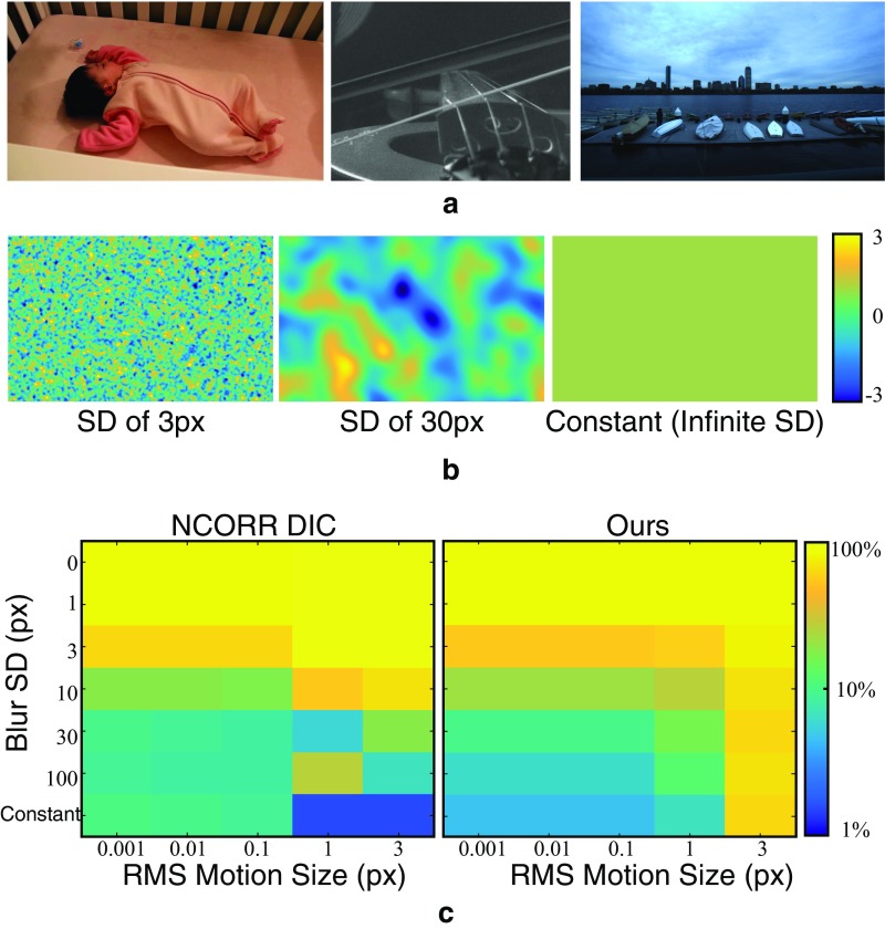
Fig. S5.
An evaluation of our motion estimation method and Ncorr (30) on a synthetic dataset of images. (A) Sample frames from real videos used to create the dataset. (B) Sample of synthetic motion fields of various motion size and spatial scale used to create the dataset. (C) The motion microscope and Ncorr are used to estimate the motion field, and the average relative error is displayed for both methods as a function of motion size and spatial scale. Both methods are only accurate for spatially smooth motion fields. Our method is twice as accurate for spatially smooth, subpixel motion fields. Ncorr is more accurate for larger motions.
For a still camera, the sensitivity of the motion microscope is mostly limited by local contrast and camera noise—fluctuations of pixel intensities present in all videos (5). When the video is motion-magnified, this noise can lead to spurious motions, especially at low-contrast edges and textures (Fig. S6). We measure motion noise level by computing the covariance matrix of each estimated motion vector. Estimating this directly from the input video is usually impossible, because it requires observing the motions without noise. We solve this by creating a simulated noisy video with zero motion, replicating a static frame of the input video and adding realistic, independent noise to each frame. We compute the sample covariance of the estimated motion vectors in this simulated video (Fig. S7 and Noise Model and Creating Synthetic Video). We show analytically, and via experiments in which the motions in a temporal band are known to be zero, that these covariance matrices are accurate for real videos (Analytic Justification of Noise Analysis and Figs. S8 and S9). We also analyze the limits of our technique by comparing to a laser vibrometer and show that, with a Phantom V-10 camera, at a high-contrast edge, the smallest motion we can detect is on the order of 1/100th of a pixel (Fig. 1 and Fig. S4).
Fig. S6.
Magnification of a spatial smooth and temporally filtered noise can look like a real signal. (A) Frames and time slices from a synthetic 300-frame video created by replicating a single frame 300 times and adding a different realistic noise pattern to each frame. (B) Corresponding frame and time slices from the synthetic video motion magnified 600 in a temporal band of 40 Hz to 60 Hz. Time slices from the same parts of each video are shown on the right for comparison.
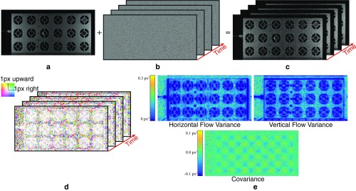
Fig. S7.
Using a probabilistic simulation to compute the noise covariance of the motion estimate. (A) A single frame from an input video, in this case, of an elastic metamaterial. (B) Simulated, but realistic noise (contrast enhanced 80). (C) Synthetic video with no motions, consisting of the input frame replicated plus simulated noise (noise contrast-enhanced 80). (D) Estimated motions of this video. (E) Sample variances and sample covariance of the vertical and horizontal components of the motion are computed to give an estimate of how much noise is in the motion estimate.
Fig. S8.
Synthetic experiments showing that our noise covariance estimation, which assumes that the motions are zero, is also accurate for small nonzero motions. (A) The motion between synthetic frames with noise and slightly translated versions (not shown) are computed over 4,000 runs at the marked point in red for several different translation amounts. Each time, different but independent noise is added to the frames. (B) The sample covariance vs. motion size. (C) Relative error of horizontal variance vs. motion size. (D) Relative error of vertical variance vs. motion size. C and D are on the same color scale.
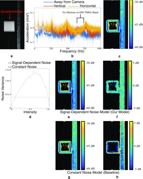
Fig. S9.
Validation of our noise estimation on real data. (A) A frame from a real video of an accelerometer attached to a beam. (B) The accelerometer shows there are no motions in the frequency band 600 Hz to 700 Hz. (C) The variance of our motion estimate in the 600- to 700-Hz band serves as a ground-truth measure of noise, as there are no motions. (D) The estimated noise level vs. intensity for a signal-dependent noise model and a constant noise model. (E) The noise estimate produced by our Monte Carlo simulation with a signal-dependent model. All variances are of the motions projected onto the direction of least variance. Textureless regions, where the motion estimation is not meaningful, have been masked out in black. (F) Difference in decibels between ground truth and E. (G) Noise estimate produced by the Monte Carlo simulation with a constant noise model. (H) Difference in decibels between ground truth and G.
Relation Between Local Phase Differences and Motions
Fleet and Jepson have shown that contours of constant phase in image subbands such as those in the complex steerable pyramid approximately track the motion of objects in a video (7). We make a similar phase constancy assumption, in which the following equation relates the phase of the frame at time to the phase of future frames:
| [S1] |
where is the motion we seek to compute. We Taylor-expand the right-hand side around to get
| [S2] |
where , arguments have been suppressed and represents higher order terms in the Taylor expansion. Because we assume the motions are small, higher order terms are negligible and the local phase variations are approximately equal to only the linear term,
| [S3] |
Fleet has shown that the spatial gradients of the local phase, , are roughly constant within a subband and that they are approximately equal to the peak tuning frequency of the corresponding subband’s filter (33). This frequency is a 2D vector oriented orthogonal to the direction the subband selects for, which means that the local phase changes only provide information about the motions perpendicular to this direction.
Noise Model and Creating Synthetic Video
We adopt a signal-dependent noise model, in which each pixel is contaminated with spatially independent Gaussian noise with variance , where is the pixel’s mean intensity (26, 34). Liu et al. (26) refer to this function as a “noise level function,” and we do the same. This reflects that sensor noise is well modeled by the sum of zero-mean Gaussian noise sources, some of which have variances that depend on intensity (5). We show that this noise model is an improvement over a constant variance noise model in Fig. S9.
The noise level function is estimated from temporal variations in the input video, with observed intensities . Assuming that is the sum of noiseless intensity and a zero-mean Gaussian noise term with variance , the temporal variations are given by the following Taylor expansion:
| [S17] |
| [S18] |
| [S19] |
The second equality is the brightness constancy assumption of optical flow (35, 36). We exclude pixels where the spatial gradient has high magnitude from our analysis. At the remaining pixel, temporal variations in are mostly due to noise,
| [S20] |
At these pixels, we take the temporal variance and mean of , which, in expectation, are and , respectively. To increase robustness, we divide the intensity range into 64 equally sized bins. For each bin, we take all those pixels with mean inside that bin and take the mean of the corresponding temporal variances of to estimate the noise level function .
With in hand, we can take frames from existing videos and use them to create simulated videos with realistic noise, but with known, zero motion. In Fig. S6A, we take a frame from a video of the metamaterial, filmed with a Phantom V-10, and add noise to it via the equation
| [S21] |
where now is Gaussian noise with unit variance. We motion-magnify the resulting video 600 times in a 20-Hz band centered at 50 Hz to show that motion-magnified noise can cause spurious motions (Fig. S6B).
We use the same simulation to create synthetic videos with which to estimate the covariance matrix of the motion vectors.
We quantify the noise in the motion vectors by estimating their covariance matrices . These matrices reflect variations in the motion caused by noise. It is not usually possible to directly estimate them from the input video, because both motions and noise vary across frames and the true motions are unknown. Therefore, we create a noisy, synthetic video with known zero true motion (Eq. S21 and Fig. S7 A–C).
We estimate the motions in (Fig. S7D) using our technique with spatial smoothing, but without temporal filtering, which we handle in a later step. This results in a set of 2D motion vectors , in which all temporal variations in are due to noise. The sample covariance matrix over the time dimension is
| [S22] |
where is the mean over of the motion vectors. is a symmetric matrix, defined at every pixel, with only three unique components. In Fig. S7E, we show these components, the variances of the horizontal and vertical components of the motion, and their covariance.
The motion projected onto a direction vector is and has variance . Of particular interest is the direction of least variance that minimizes . In the case of an edge in the image, the direction of least variance is usually normal to the edge.
Analytic Justification of Noise Analysis
We analyze only the case when the amplitudes at a pixel in all subbands are large (), because the local phases have a Gaussian distribution in this case. Such points intuitively correspond to places where there is image content in at least two directions. In this case, we show that the sample covariance matrix computed using a simulated video with no motions is accurate for videos with subpixel small motions.
We reproduce the linearization of phase constancy equation (Eq. S3) with noise terms added to the phase variations () and phase gradient (),
| [S23] |
The total noise term in this equation is . The noise terms , and are of the same order of magnitude. Since and are much less than pixel, the predominant source of noise is from , the effects of and are negligible, and we can ignore them, allowing us to write the noisy version of the equation as
| [S24] |
The motion estimate is the solution to a weighted least squares problem, . To simplify notation, let , the parts of the equation that don’t depend on time. Then, the flow estimate is
| [S25] |
where the elements of are the local phase variations over time. and contain the spatial gradients of phase and amplitude, respectively. We have demonstrated that is close to noiseless (Eq. S24), and our assumption about the amplitudes being large means is also approximately noiseless, which means that is noiseless.
We split into the sum of its mean and variance, a multivariate Gaussian random variable, denoted as , that has zero mean and variance that depends only on image noise and local image content. Then, the flow estimate is
| [S26] |
The noise term doesn’t depend on the value of the true flow . Therefore, the estimated covariance matrix is valid even when the motions are nonzero but small.
From Eq. S15, we know that is proportional to the amount of sensor noise. Therefore, an interesting consequence of Eq. S26 is that the motion covariance matrix will be linearly proportional to the variance of the sensor noise.
Results and Discussion
We applied the motion microscope to several problems in biology and engineering. First, we used it to reveal one component of the mechanics of hearing. The mammalian cochlea is a remarkable sensor that can perform high-quality spectral analysis to discriminate as many as 30 frequencies in the interval of a semitone (8). These extraordinary properties of the hearing organ depend on traveling waves of motion that propagate along the cochlear spiral. These wave motions are coupled to the extremely sensitive sensory receptor cells via the tectorial membrane, a gelatinous structure that is 97% water (9).
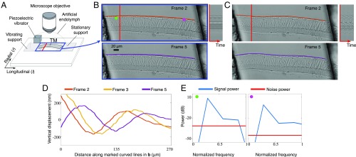
To better understand the functional role of the tectorial membrane in hearing, we excised segments of the tectorial membrane from a mouse cochlea and stimulated it with audio frequency vibrations (Movie S1 and Fig. 2A). Prior work suggested that motions of the tectorial membrane would rapidly decay with distance from the point of stimulation (10). The unprocessed video of the tectorial membrane appeared static, making it difficult to verify this. However, when the motions were amplified 20 times, waves that persisted over hundreds of micrometers were revealed (Movie S1 and Fig. 2 B–E).
Fig. 2.
Exploring the mechanical properties of a mammalian tectorial membrane with the motion microscope. (A) The experimental setup used to stroboscopically film a stimulated mammalian tectorial membrane (TectaY1870C/+). Subfigure Copyright (2007) National Academy of Sciences of the United States of America. Reproduced from ref. 12. (B) Two of the eight captured frames . (Movie S1, data previously published in ref. 13). (C) Corresponding frames from the motion-magnified video in which displacement from the mean was magnified 20. The orange and purple lines on top of the tectorial membrane in B are warped according to magnified motion vectors to produce the orange and purple lines in C. (D) The vertical displacement along the orange and purple lines in B is shown for three frames. (E) The power spectrum of the motion signal and noise power is shown in the direction of least variance at the magenta and green points in B.
Subpixel motion analysis suggests that these waves play a prominent role in determining the sensitivity and frequency selectivity of hearing (11–14). Magnifying motions has provided new insights into the underlying physical mechanisms of hearing. Ultimately, the motion microscope could be applied to see and interpret the nanoscale motions of a multitude of biological systems.
We also applied the motion microscope to the field of modal analysis, in which a structure’s resonant frequencies and mode shapes are measured to characterize its dynamic behavior (15). Common applications are to validate finite element models and to detect changes or damage in structures (16). Typically, this is done by measuring vibrations at many different locations on the structure in response to a known input excitation. However, approximate measurements can be made under operational conditions assuming broadband excitation (17). Contact accelerometers have been traditionally used for modal analysis, but densely instrumenting a structure can be difficult and tedious, and, for light structures, the accelerometers’ mass can affect the measurement.
The motion microscope offers many advantages over traditional sensors. The structure is unaltered by the measurement, the measurements are spatially dense, and the motion-magnified video allows for easy interpretation of the motions. While only structural motions in the image plane are visible, this can be mitigated by choosing the viewpoint carefully.
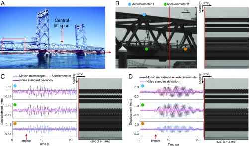
We applied the motion microscope to modal analysis by filming the left span of a suspension bridge from 80 m away (Fig. 3A). The central span was lowered and impacted the left span. Despite this, the left span looks completely still in the input video (Fig. 3B). Two of its modal shapes are revealed in Movie S2 when magnified 400 (1.6 Hz to 1.8 Hz) and 250 (2.4 Hz to 2.7 Hz). In Fig. 3 C and D, we show time slices from the motion-magnified videos, displacements versus time at three points, and the estimated noise standard deviations. We also used accelerometers to measure the motions of the bridge at two of those points (Fig. 3B). The motion microscope matches the accelerometers within error bars. In a second example, we show the modal shapes of a pipe after it is struck with a hammer (Modal Shapes of a Pipe, Fig. S10, and Movie S3).
Fig. 3.
The motion microscope reveals modal shapes of a lift bridge. (A) The outer spans of the bridge are fixed while the central span moves vertically. (B) The left span was filmed while the central span was lowered. A frame from the resulting video and a time slice at the red line are shown. (C) Displacement and noise SD from the motion microscope are shown for motions in a 1.6- to 1.8-Hz band at the cyan, green, and orange points in B. Doubly integrated data from accelerometers at the cyan and green points are also shown. A time slice from the motion-magnified video is shown (Movie S2). The time at which the central span is fully lowered is marked as “impact.” (D) Same as C, but for motions in a 2.4- to 2.7-Hz band.
Fig. S10.
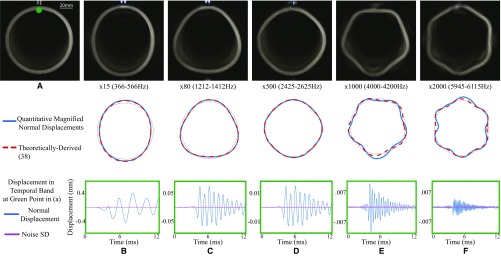
The motion microscope is applied to a pipe being struck by a hammer. (A) A frame from the input video, recorded at 24,096 FPS. (B–F) (Top) A frame is shown from five motion-magnified videos showing motions amplified in the specified frequency bands (Movie S3). (Middle) Modal shapes recovered from a quantitative analysis of the motions are shown in blue. The theoretically derived modal shapes, shown in dashed orange, are overlaid for comparison over a perfect circle in dotted black. (Bottom) Displacement vs. time and the estimated noise SD is shown at the green point marked in A.
In our final example, we used the motion microscope to verify the functioning of elastic metamaterials, artificially structured materials designed to manipulate and control the propagation of elastic waves. They have received much attention (18) because of both their rich physics and their potential applications, which include wave guiding (19), cloaking (20), acoustic imaging (21), and noise reduction (22). Several efforts have been made to experimentally characterize the elastic wave phenomena observed in these systems. However, as the small amplitude of the propagating waves makes it impossible to directly visualize them, the majority of the experimental investigations have focused on capturing the band gaps through the use of accelerometers, which only provide point measurements. Visualizing the mechanical motions everywhere in the metamaterials has only been possible using expensive and highly specialized setups like scanning laser vibrometers (23).
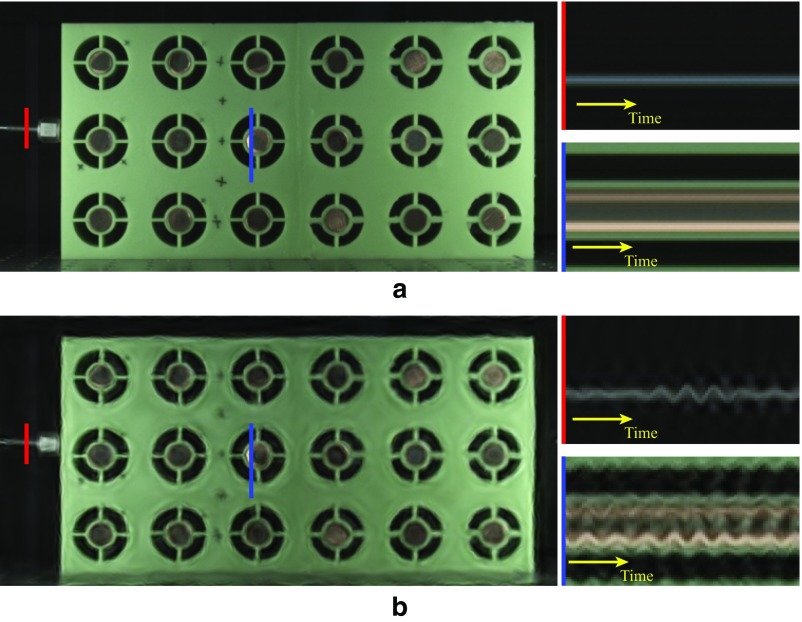
We focus on a metamaterial comprising an elastic matrix with embedded resonating units, which consists of copper cores connected to four elastic beams (24). Even when vibrated, this metamaterial appears stationary, making it difficult to determine if the metamaterial is functioning correctly (Movies S4 and S5). Previously, these miniscule vibrations were measured with two accelerometers (24). This method only provides point measurements, making it difficult to verify the successful attenuation of vibrations. We gain insight and understanding of the system by visually amplifying its motion.
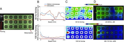
The elastic metamaterial was forced at two frequencies, 50 Hz and 100 Hz, and, in each case, it was filmed at 500 frames per second (FPS) (Fig. 4A). The motions in 20-Hz bands around the forcing frequencies were amplified, revealing that the metamaterial functions as expected (24), passing 50-Hz waves and rapidly attenuating 100-Hz waves (Movies S4 and S5). We also compared our results with predictions from a finite element analysis simulation (Fig. 4 B and C). In Fig. 4D, we show heatmaps of the estimated displacement amplitudes overlaid on the motion-magnified frames. We interpolated displacements into textureless regions, which had noisy motion estimates. The agreement between the simulation (Fig. 4C) and the motion microscope (Fig. 4D) demonstrates the motion microscope’s usefulness in verifying the correct function of the metamaterial.
Fig. 4.
The motion microscope is used to investigate properties of a designed metamaterial. (A) The metamaterial is forced at 50 Hz and 100 Hz in two experiments, and a frame from the 50-Hz video is shown. (B) One-dimensional slices of the displacement amplitude along the red line in A are shown for both a finite element analysis simulation and the motion microscope. (C) A finite element analysis simulation of the displacement of the metamaterial. Color corresponds to displacement amplitude, and the material is warped according to magnified simulated displacement vectors. (D) Results from the motion microscope are shown. Displacement magnitudes are shown in color at every point on the metamaterial, overlayed on frames from the motion-magnified videos (Movies S4 and S5).
Modal Shapes of a Pipe
We made a measurement of a pipe being struck by a hammer, viewed end on by a camera, to capture its radial–circumferential vibration modes. A standard schedule 40 PVC pipe was recorded with a high-speed camera at 24,000 FPS, at a resolution of 192 192 (Fig. S10A). Fig. S10 B–F shows frames from the motion-magnified videos for different resonant frequencies showing the mode shapes, a comparison of the quantitatively measured mode shapes with the theoretically derived mode shapes, and the displacement vs. time of the specific frequency band and the estimated noise SD. The tiny modal motions are seen clearly. Obtaining vibration data with traditional sensors with the same spatial density would be extremely difficult, and accelerometers placed on the pipe would alter its resonant frequencies.
This sequence also demonstrates the accuracy of our noise analysis. The noise standard deviations show that the detected motions before impact, when the pipe is stationary, are likely spurious.
Synthetic Validation
We validate the accuracy of our motion estimation on a synthetic dataset and compare its accuracy to Ncorr, a digital image correlation technique (30) used by mechanical engineers (31). In this experiment, we did not use temporal filtering.
We created a synthetic dataset of frame pairs with known ground-truth motions between them. We took natural images from the frames of real videos (Fig. S5A) and warped them according to known motion fields using cubic b-spline interpolation (32). Sample motions fields, shown in Fig. S5B, were produced by Gaussian-blurring IID Gaussian random variables. We used Gaussian blurs with SDs, ranging from zero (no filtering) to infinite (a constant motion field). We also varied the RMS amplitude of the motion fields from 0.001 pixels to three pixels. For each set of motion field parameters, we sampled five different motion fields to produce a total of 155 motion fields with different amplitudes and spatial coherence. To test the accuracy of the algorithms rather than their sensitivity to noise, no noise was added to the image pairs.
We ran our motion estimation technique and Ncorr on each image pair. We then computed the mean absolute difference between the estimated and ground-truth motion fields. Then, for each set of motion field parameters, we averaged the mean absolute differences across image pairs and divided the result by the RMS motion amplitude to make the errors comparable over motion sizes. The result is the average relative error as a percentage of RMS motion amplitude (Fig. S5C).
Both Ncorr and our method perform best when the motions are spatially coherent (filter standard deviations greater than 10 pixels) with relative errors under 10%. This reflects the fact that both methods assume the motion field is spatially smooth. Across motion sizes, our method performs best for subpixel motions (5% relative error). This is probably because we assume that the motions are small when we linearize the phase constancy equation (Eq. S3). Ncorr has twice the relative error (10%) for the same motion fields.
The relative errors reported in Fig. S5C are computed over all pixels, including those that are in smooth, textureless regions where it is difficult to estimate the motions. If we restrict the error metric to only take into account pixels at edges and corners, the average relative errors for small ( pixel RMS), spatially coherent (filter SD pixels) motions drops by a factor of 2.5 for both methods.
We generated synthetic images that are slight translations of each other and added Gaussian noise to the frames (Fig. S8A). For each translation amount, we compute the motion between the two frames over 4,000 runs. We compute the sample covariance matrix over the runs as a measure of the ground-truth noise level. We also used our noise analysis to estimate the covariance matrix at the points denoted in red.
The off-diagonal term of the covariance matrix should be zero for the synthetic frames in Fig. S8A. For both examples, it is within square pixels of zero for all translation amounts (Fig. S8B).
The relative errors of the horizontal and vertical variances vs. translation (Fig. S8 C and D) are less than for subpixel motions. This is likely due to the random nature of the simulation. For motions greater than one pixel, the covariance matrix has a relative error of less than .
Low-Amplitude Coefficients Have Noisy Phase
Each frame of the input video is transformed to the complex steerable pyramid representation by being spatially band-passed by a bank of quadrature pairs of filters and , where corresponds to different spatial scales of the pyramid and corresponds to different orientations. We use the filters of Portilla and Simoncelli, which are specified and applied in the frequency domain (25). For one such filter pair, the result is a set of complex coefficients whose real and imaginary part are given by
| [S4] |
where the convolution is applied spatially at each time instant . This filter pair is converted to amplitude and phase by the operations
| [S5] |
Filters and are in quadrature relationship, which means that they select for the same frequencies, but are 90 degrees out of phase like and . A consequence is that they are uncorrelated and have equal RMS values. Complex coefficients at antipodal orientations are conjugate symmetric and contain redundant information. Therefore, we only use a half-circle of orientations.
Suppose the observed video is contaminated with IID noise of variance ,
| [S6] |
where is the underlying noiseless video. This noise causes the complex steerable pyramid coefficients to be noisy, which causes the local phase to be noisy. We show that the local phase at a point has an approximate Gaussian distribution when the amplitude is high and is approximately uniformly distributed when the amplitude is low.
The transformed representation has response
| [S7] |
The first term in each expression is the noiseless filter response, which we denote for the real part and for the imaginary part. The second term in each expression is filtered noise, which we denote as and . At a single point, and are Gaussian random variables with covariance matrix equal to
| [S8] |
where is the identity matrix and equality follows from the fact that and are quadrature pairs.
We suppress the indices in this section for readability. From Eq. S5, the noiseless and noisy phases are given by
| [S9] |
Their difference linearized around is
| [S10] |
The terms and are expected to be equal to their variance . Therefore, if , higher order terms are negligible. In this case, we see that the phase is approximately a linear combination of Gaussian random variables and is therefore Gaussian. This is illustrated empirically by local phase histograms of the green and blue points in Fig. S3 A–E.
For these high-amplitude points, we compute the variance of the phase of a coefficient,
| [S11] |
| [S12] |
| [S13] |
| [S14] |
| [S15] |
The first approximation follows from the linearization of Eq. S10.
When the amplitude is low compared with the noise level (), the linearization of Eq. S10 is not accurate. In this case, and , and phase is given by
| [S16] |
and are uncorrelated Gaussian random variables with equal variance, which means that the phase is a uniformly random number. The phase at such points contains no information and intuitively corresponds to places where there is no image content in a given pyramid level (Fig. S3E, red point).
Conclusion
Small motions can reveal important dynamics in a system under study, or can foreshadow large-scale motions to come. Motion microscopy facilitates their visualization, and has been demonstrated here for motion amplification factors from 20 to 400 across length scales ranging from 100 nm to 0.3 mm.
Materials and Methods
Quantitative Motion Estimation.
For every pixel at location and time , we combine spatial local phase information in different subbands of the frames of the input video using the least squares objective function,
| [2] |
Arguments have been suppressed for readability; and are the spatial local amplitude and phase of a steerable pyramid representation of the image, and and are the horizontal and vertical motions, respectively, at every pixel. The solution () is our motion estimate and is equal to
| [3] |
where is with th row , is with th row , and is a diagonal matrix with th diagonal element .
To increase the signal-to-noise ratio, we assume the motion field is constant in a small window around each pixel. This gives additional constraints from neighboring pixels, weighted by both their amplitude squared and the corresponding value in a smoothing kernel , to the objective described in Eq. 3. To handle temporal filtering, we replace the local phase variations with temporally filtered local phase variations.
We use a four-orientation complex steerable pyramid specified by Portilla and Simoncelli (25). We use only the two highest-frequency scales of the complex steerable pyramid, for a total of eight subbands. We use a Gaussian spatial smoothing kernel with a SD of 3 pixels and a support of pixels. The temporal filter depends on the application.
Noise Model and Creating Synthetic Video.
We estimate the noise level function (26) of a video. We apply derivative of Gaussian filters to the image in the and directions and use them to compute the gradient magnitude. We exclude pixels where the gradient magnitude is above on a to intensity scale. At the remaining pixels, we take the temporal variance and mean of the image. We divide the intensity range into 64 equally sized bins. For each bin, we take all pixels with mean inside that bin and take the mean of the corresponding temporal variances of to form 64 points that are linearly interpolated to estimate the noise level function .
Estimating Covariance Matrices of Motion Vectors.
For an input video , we use the noise level function to create a synthetic video
| [4] |
that is frames long. We estimate the covariance matrices of the motion vectors by taking the temporal sample covariance of ,
| [5] |
where is the mean over of the motion vectors.
The temporal filter reduces noise and decreases the covariance matrix. Oppenheim and Schafer (27) show that a signal with independent and identically distributed (IID) noise of variance , when filtered with a filter with impulse response , has variance . Therefore, when a temporal filter is used, we multiply the covariance matrix by .
Comparison of Our Motion Estimation to a Laser Vibrometer.
We compare the results of our motion estimation algorithm to that of a laser vibrometer, which measures velocity using Doppler shift (28). In the first experiment, a cantilevered beam was shaken by a mechanical shaker at Hz, Hz, Hz, and Hz, the measured modal frequencies of the beam. The relative amplitude of the shaking signal was varied between a factor of and in increments. We simultaneously recorded a 2,000 FPS video of the beam with a high-speed camera (VisionResearch Phantom V-10) and measured its horizontal velocity with a laser vibrometer (Polytec PDV100). We repeated this experiment for nine different excitation magnitudes, three focal lengths ( mm, mm, mm) and eight exposure times ( s, s, s, s, s, s, s, s), for a total of 20 high-speed videos. The beam had an accelerometer mounted on it (white object in Fig. 1A), but we did not use it in this experiment.
We used our motion estimation method to compute the horizontal displacement of the marked, red point on the left side of the accelerometer from the video (Fig. 1A). We applied a temporal band-stop filter to remove motions between 67 Hz and 80 Hz that corresponded to camera motions caused by its cooling fan’s rotation. The laser vibrometer signal was integrated using discrete, trapezoidal integration. Before integration, both signals were high-passed above 2.5 Hz to reduce low-frequency noise in the integrated vibrometer signal. The motion signals from each video were manually aligned. For one video (exposure, s; excitation, ; and focal length, mm), we plot the two motion signals (Fig. S4 B–D). They agree remarkably well, with higher modes well aligned and a correlation of .
To show the sensitivity of the motion microscope, we plot the correlation of our motion estimate and the integrated velocities from the laser vibrometer vs. motion size (RMS displacement). Because the motion’s average size varies over time, we divide each video’s motion signal into eight equal pieces and plot the correlations of each piece in each video in Fig. S4 E and F. For RMS displacements on the order of th of a pixel, the correlation between the two signals varies between and . For motions larger than th of a pixel, the correlation is between and . Possible sources of discrepancy are noise in the motion microscope signal, integrated low-frequency noise in the vibrometer signal, and slight misalignment between the signals. Displacements with RMS smaller than th of a pixel were noisier and had lower correlations, indicating that noise in the video prevents the two signals from matching.
As expected, correlation increases with focal length and excitation magnitude, two things that positively correlate with motion size (in pixels) (Fig. S4 G and H). The correlation also increases with exposure, because videos with lower exposure times are noisier (Fig. S4I).
Filming Bridge Sequence.
The bridge was filmed with a monochrome Point Gray Grasshopper3 camera (model GS3-U3-23S6M-C) at 30 FPS with a resolution of 800 600. The central span of the bridge lifted to accommodate marine traffic. Filming was started about 5 s before the central span was lowered to its lowest point.
The accelerometer data were doubly integrated using trapezoidal integration to displacement. In Fig. 3 C and D, both the motion microscope displacement and the doubly integrated acceleration were band-passed with a first-order band-pass Butterworth filter with the specified parameters.
Motion Field Interpolation.
In textureless regions, it may not be possible to estimate the motion at all, and, at one-dimensional structures like edges, the motion field will only be accurate in the direction perpendicular to the edge. These inaccuracies are reflected in the motion covariance matrix. We show how to interpolate the motion field from accurate regions to inaccurate regions, assuming that adjacent pixels have similar motions.
We minimize the following objective function:
| [6] |
where is the desired interpolated field, is the estimated motion field, is its covariance, is the four-pixel neighborhood of , and is a user-specified constant that specifies the relative importance of matching the estimated motion field vs. making adjacent pixels have similar motion fields. The first term seeks to ensure that is close to , weighted by the expected amount of noise at each pixel. The second term seeks to ensure that adjacent pixels have similar motion fields.
In Fig. 4D, we produce the color overlays by applying the above processing to the estimated motion field with and then taking the amplitude of each motion vector. We also set components of the covariance matrix that were larger than square pixels to be an arbitrarily large number (we used square pixels).
Finite Element Analysis of Acoustic Metamaterial.
We use Abaqus/Standard (29), a commercial finite-element analyzer, to simulate the metamaterial’s response to forcing. We constructed a 2D model with 37,660 nodes and 11,809 eight-node plane strain quadrilateral elements (Abaqus element type CPE8H). We modeled the rubber as Neo-Hookean, with shear modulus kPa, bulk modulus kPa, and density (Abaqus parameters kPa, ). We modeled the copper core with shear modulus , bulk modulus , and density (Abaqus parameters , . Geometry and material properties are specified in Wang et al. (24). The bottom of the metamaterial was given a zero-displacement boundary condition. A sinusoidal displacement loading condition at the forcing frequency was applied to a node located halfway between the top and bottom of the metamaterial.
Validation of Noise Analysis with Real Video Data.
We took a video of an accelerometer attached to a beam (Fig. S9A). We used the accelerometer to verify that the beam had no motions between 600 Hz and 700 Hz (Fig. S9B). We then estimated the in-band motions from a video of the beam. Because the beam is stationary in this band, these motions are entirely due to noise, and their temporal sample covariance gives us a ground-truth measure of the noise level (Fig. S9C). We used our simulation with a signal-dependent noise model to estimate the covariance matrix from the first frame of the video, the specific parameters of which are shown in Fig. S9D. The resulting covariance matrices closely match the ground truth (Fig. S9 E and F), showing that our simulation can accurately estimate noise level and error bars.
We also verify that the signal-dependent noise model performs better than the simpler constant variance noise model, in which noise is IID. The result of the constant noise model simulation produced results that are much less accurate than the signal-dependent noise model (Fig. S9 G and H).
In Fig. S9, we only show the component of the covariance matrix corresponding to the direction of least variance, and only at points corresponding to edges or corners.
Using the Motion Microscope and Limitations
The motion microscope works best when the camera is stable, such as when mounted on a tripod. If the camera is handheld or the tripod is not sturdy, the motion microscope may only detect camera motions instead of subject motions. The easiest way to solve this problem is to stabilize the camera. If the camera motions are caused by some periodic source, such as camera fans, that occur at a temporal frequency that the subject is not moving at, they can be removed with a band-stop filter.
If adjacent individual pixels have different motions, it is unlikely that the motion microscope will be able to discern or differentiate them. The motion microscope assumes motions are locally constant, and it won’t be able to properly process videos with high spatial frequency motions. The best way to solve this problem is to increase the resolving power or optical zoom of the imaging system. If noise is not a concern, reducing the width of the spatial Gaussian used to smooth the motions may also help.
It is not possible for the motion microscope to quantify the movement of textureless regions or the full 2D movement of 1D edges. However, the motion covariance matrices produced by the motion microscope will alert the user as to when this is happening. The visualization will still be reasonable, as it is not possible to tell if a textureless region was motion-amplified in the wrong way.
Saturated, pure white pixels may pose a problem for the motion microscope. Slight color changes are the underlying signal used to detect tiny motions. For pixels with clipped intensities, this signal will be missing, and it may not be possible to detect motion. The best ways to mitigate this problem are to reduce the exposure time, change the position of lights, or use a camera with a higher dynamic range.
The motion microscope only quantifies lateral, 2D motions in the imaging plane. Motions of the subject toward or away from the camera will not be properly reported. For a reasonable camera, these 2D motions can be multiplied by a constant to convert from pixels to millimeters or other units of interest. However, if the lens has severe distortion, the constant will vary across the scene. If quantification of the motions is important, the images will need to be lens distortion-corrected before the motion microscope is applied.
The motion microscope visualization is unable to push pixels beyond the support of the basis functions of the steerable pyramid. In practice, this results in a maximum amplified motion of around four pixels. If the amplification is high enough to push an image feature past this, ringing artifacts may occur.
Supplementary Material
Acknowledgments
We thank Professor Erin Bell and Travis Adams at University of New Hampshire and New Hampshire Department of Transportation for their assistance with filming the Portsmouth lift bridge. This work was supported, in part, by Shell Research, Quanta Computer, National Science Foundation Grants CGV-1111415 and CGV-1122374, and National Institutes of Health Grant R01-DC00238.
Footnotes
The authors declare no conflict of interest.
This article is a PNAS Direct Submission.
This article contains supporting information online at www.pnas.org/lookup/suppl/doi:10.1073/pnas.1703715114/-/DCSupplemental.
References
- 1.Liu C, Torralba A, Freeman WT, Durand F, Adelson EH. Motion magnification. ACM Trans Graph. 2005;24:519–526. [Google Scholar]
- 2.Wu HY, et al. Eulerian video magnification for revealing subtle changes in the world. ACM Trans Graph. 2012;31:1–8. [Google Scholar]
- 3.Wadhwa N, Rubinstein M, Durand F, Freeman WT. Phase-based video motion processing. ACM Trans Graph. 2013;32:80. [Google Scholar]
- 4.Wadhwa N, Rubinstein M, Durand F, Freeman WT. IEEE International Conference on Computational Photography. Inst Electr Electron Eng; New York: 2014. Riesz pyramid for fast phase-based video magnification; pp. 1–10. [Google Scholar]
- 5.Nakamura J. Image Sensors and Signal Processing for Digital Still Cameras. CRC; Boca Raton, FL: 2005. [Google Scholar]
- 6.Simoncelli EP, Freeman WT. The steerable pyramid: A flexible architecture for multi-scale derivative computation. Int J Image Proc. 1995;3:444–447. [Google Scholar]
- 7.Fleet DJ, Jepson AD. Computation of component image velocity from local phase information. Int J Comput Vis. 1990;5:77–104. [Google Scholar]
- 8.Dallos P, Fay RR. 2012. The Cochlea, Springer Handbook of Auditory Research (Springer Science, New York), Vol 8.
- 9.Thalmann I. Collagen of accessory structures of organ of Corti. Connect Tissue Res. 1993;29:191–201. doi: 10.3109/03008209309016826. [DOI] [PubMed] [Google Scholar]
- 10.Zwislocki JJ. Five decades of research on cochlear mechanics. J Acoust Soc Am. 1980;67:1679–1685. doi: 10.1121/1.384294. [DOI] [PubMed] [Google Scholar]
- 11.Sellon JB, Farrahi S, Ghaffari R, Freeman DM. Longitudinal spread of mechanical excitation through tectorial membrane traveling waves. Proc Natl Acad Sci USA. 2015;112:12968–12973. doi: 10.1073/pnas.1511620112. [DOI] [PMC free article] [PubMed] [Google Scholar]
- 12.Ghaffari R, Aranyosi AJ, Freeman DM. Longitudinally propagating traveling waves of the mammalian tectorial membrane. Proc Natl Acad Sci USA. 2007;104:16510–16515. doi: 10.1073/pnas.0703665104. [DOI] [PMC free article] [PubMed] [Google Scholar]
- 13.Sellon JB, Ghaffari R, Farrahi S, Richardson GP, Freeman DM. Porosity controls spread of excitation in tectorial membrane traveling waves. J Biophys. 2014;106:1406–1413. doi: 10.1016/j.bpj.2014.02.012. [DOI] [PMC free article] [PubMed] [Google Scholar]
- 14.Ghaffari R, Aranyosi AJ, Richardson GP, Freeman DM. Tectorial membrane traveling waves underlie abnormal hearing in tectb mutants. Nat Commun. 2010;1:96. doi: 10.1038/ncomms1094. [DOI] [PMC free article] [PubMed] [Google Scholar]
- 15.Ewins DJ. 1995. Modal Testing: Theory and Practice, Engineering Dynamics Series (Res Stud, Baldock, UK) Vol 6.
- 16.Salawu O. Detection of structural damage through changes in frequency: A review. Eng Struct. 1997;19:718–723. [Google Scholar]
- 17.Hermans L, van der Auweraer H. Modal testing and analysis of structures under operational conditions: Industrial applications. Mech Sys Signal Process. 1999;13:193–216. [Google Scholar]
- 18.Hussein MI, Leamy MJ, Ruzzene M. Dynamics of phononic materials and structures: Historical origins, recent progress, and future outlook. Appl Mech Rev. 2014;66:040802. [Google Scholar]
- 19.Khelif A, Choujaa A, Benchabane S, Djafari-Rouhani B, Laude V. Guiding and bending of acoustic waves in highly confined phononic crystal waveguides. Appl Phys Lett. 2004;84:4400–4402. [Google Scholar]
- 20.Cummer S, Schurig D. One path to acoustic cloaking. New J Phy. 2007;9:45. [Google Scholar]
- 21.Spadoni A, Daraio C. Generation and control of sound bullets with a nonlinear acoustic lens. Proc Natl Acad Sci USA. 2010;107:7230–7234. doi: 10.1073/pnas.1001514107. [DOI] [PMC free article] [PubMed] [Google Scholar]
- 22.Elser D, et al. Reduction of guided acoustic wave Brillouin scattering in photonic crystal fibers. Phys Rev Lett. 2006;97:133901. doi: 10.1103/PhysRevLett.97.133901. [DOI] [PubMed] [Google Scholar]
- 23.Jeong S, Ruzzene M. Experimental analysis of wave propagation in periodic grid-like structures. Proc SPIE. 2005;5760:518–525. [Google Scholar]
- 24.Wang P, Casadei F, Shan S, Weaver JC, Bertoldi K. Harnessing buckling to design tunable locally resonant acoustic metamaterials. Phys Rev Lett. 2014;113:014301. doi: 10.1103/PhysRevLett.113.014301. [DOI] [PubMed] [Google Scholar]
- 25.Portilla J, Simoncelli EP. A parametric texture model based on joint statistics of complex wavelet coefficients. Int J Comput Vis. 2000;40:49–70. [Google Scholar]
- 26.Liu C, Freeman WT, Szeliski R, Kang SB. 2006 IEEE Computer Society Conference on Computer Vision and Pattern Recognition. Inst Electr Electron Eng; New York: 2006. Noise estimation from a single image; pp. 901–908. [Google Scholar]
- 27.Oppenheim AV, Schafer RW. Discrete-Time Signal Processing. Prentice Hall; New York: 2010. [Google Scholar]
- 28.Durst F, Melling A, Whitelaw JH. 1976. Principles and Practice of Laser-Doppler Anemometry. NASA STI/Recon Technical Report A (NASA, Washington, DC), vol 76.
- 29. Hibbett, Karlsson, Sorensen (1998) ABAQUS/Standard: User’s Manual (Hibbitt, Karlsson & Sorensen, Pawtucket, RI) Vol 1.
- 30.Blaber J, Adair B, Antoniou A. Ncorr: Open-source 2D digital image correlation MATLAB software. Exp Mech. 2015;55:1105–1122. [Google Scholar]
- 31.Xu J, Moussawi A, Gras R, Lubineau G. Using image gradients to improve robustness of digital image correlation to non-uniform illumination: Effects of weighting and normalization choices. Exp Mech. 2015;55:963–979. [Google Scholar]
- 32.Unser M. Splines: A perfect fit for signal and image processing. Signal Process Mag. 1999;16:22–38. [Google Scholar]
- 33.Fleet DJ. Measurement of Image Velocity. Kluwer Acad; Norwell, MA: 1992. [Google Scholar]
- 34.Hasinoff SW, Durand F, Freeman WT. 2010 IEEE Computer Society Conference on Computer Vision and Pattern Recognition. Inst Electr Electron Eng; New York: 2010. Noise-optimal capture for high dynamic range photography; pp. 553–560. [Google Scholar]
- 35.Lucas BD, Kanade T. An iterative image registration technique with an application to stereo vision. Int Joint Conf Artif Intell. 1981;81:674–679. [Google Scholar]
- 36.Horn B, Schunck B. Determining optical flow. Artif Intell. 1981;17:185–203. [Google Scholar]
- 37.Wadhwa N, et al. Eulerian video magnification and analysis. Commun ACM. 2016;60:87–95. [Google Scholar]
- 38.Wachel JC, Morton SJ. Proceedings of the 19th Turbomachinery Symposium. Atkins KE (1990) Piping vibration analysis. pp. 119–134. [Google Scholar]
Associated Data
This section collects any data citations, data availability statements, or supplementary materials included in this article.


