Coupled dynamics of body mass and population growth in response to environmental change

Abstract

Environmental change has altered the phenology, morphological traits and population dynamics of many species^1,2. However, the links underlying these joint responses remain largely unknown due to a paucity of long-term data and the lack of an appropriate analytical framework³. Here, we investigate the link between phenotypic and demographic responses to environmental change using a novel methodology and an exceptional long-term (1976–2008) dataset from a hibernating mammal (the yellow-bellied marmot) inhabiting a dynamic subalpine habitat. We demonstrate how earlier emergence from hibernation and earlier weaning of young has led to a longer growing season and larger body masses prior to hibernation. The resulting shift in both the phenotype and the relationship between phenotype and fitness components led to a decline in adult mortality, which in turn triggered an abrupt increase in population size in recent years. Direct and trait-mediated effects of environmental change had comparable contributions to the observed dramatic increase in population growth. Our results help explain how a shift in phenology can cause simultaneous phenotypic and demographic changes, and highlight the need for a theory integrating ecological and evolutionary dynamics in stochastic environments^4,5.

Rapid environmental change, largely attributed to anthropogenic influences, is occurring at an unprecedented rate^6,7. Concurrent with environmental change, there have been changes in the phenology⁸, geographic distribution⁹, phenotypic trait distributions and population dynamics¹⁰ of wildlife species, particularly those living in extreme environments including high altitude or latitude ecosystems^2,11. However, the proximate causes that generate such change are rarely identified, and most analyses are phenomenological². Population-level responses to environmental change can be of several types: genetic changes occur as a result of directional selection on heritable traits or drift^12,13; life-history and quantitative traits can shift as a result of both a plastic response to environmental change^14,15 and changing selection pressures^16–18; and population size can change with changing demographic rates^19,20. Each of these processes depend on the association between phenotypic traits and survival, reproduction, trait development among survivors and the distribution of traits among newborns²¹. Understanding the effects of environmental change on populations consequently requires insight into how phenotype-demography relationships are altered and how these changes affect the distribution of phenotypic traits, life-history and population growth^22,23.

In this study, we use a long-term dataset from a hibernating sciurid rodent inhabiting a subalpine habitat to investigate how environmental change has affected phenotypic traits and population dynamics (Fig. S1). We used 33 years (1976–2008) of individual-based life-history and body mass data collected from a yellow-bellied marmot (Marmota flaviventris) population located in the Upper East River Valley, Colorado, USA. We used data only from the female segment of the population because maternity, unlike paternity, is known with confidence for each pup and most males disperse by the end of their second year. We focus on body mass as the focal phenotypic trait, because marmot life-history, particularly survival during hibernation and reproduction upon emergence, is heavily dependent on this trait^24,25.

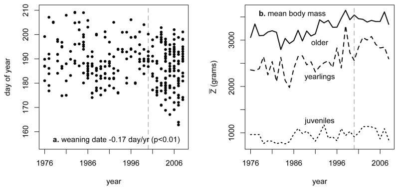
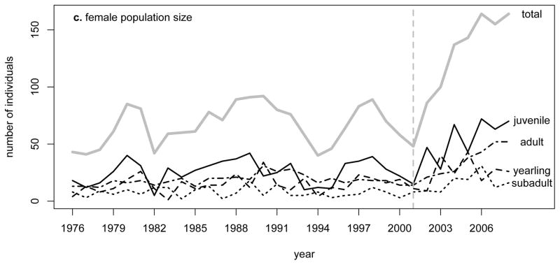
Climate change has influenced several aspects of marmot phenology⁸. Marmots have been emerging earlier from hibernation⁸ and giving birth earlier in the season (Fig. 1A), which allowed individuals more time to grow until immergence into hibernation. Using body mass measurements from repeated captures during each summer and mixed-effects models, we estimated August 1^st body mass for each individual in the population in each year (Fig. S2). Despite annual fluctuations, there has been a shift in the mean body mass in older age classes; for example, the mean body mass for 2 year-old and older adults has increased from 3094.4 g (SE = 28.9) during the first half of the study to 3433.0 g (SE = 28.0) during the second half (Fig. 1B). Meanwhile, population size has fluctuated around a stable equilibrium until 2001, followed by a steady increase during the last seven years (Fig. 1C). A non-linear (weighted) least-squares analysis indicated a break-point in population dynamics at year 2000.9 (SE = 1.12, p < 0.001). The regression slopes from this analysis reveal that the population size increased on average by 0.56 (SE = 0.45, p = 0.22) marmots/year between 1976 and 2001 and by 14.2 marmots/year subsequently (SE = 3.17, p < 0.01), indicating a major shift in the population dynamics. To examine these demographic and phenotypic changes, we compared body mass – demography associations between pre-2000 and post-2000 years. We included a one-year lag because body condition is expected to influence population size (through survival and reproduction) one year later. It is notable that the change in population growth rate occurred more suddenly than change in mean body mass (Fig. 1B–C). Nonetheless, the majority of the highest mean body masses were observed during the last decade, particularly for adults, suggesting that gradual changes in the environment may have passed a threshold leading to a gradual shift in the body mass and an abrupt shift in the demographic regime. Interestingly, other aspects of marmot habitat, including flowering rates of Tall Bluebell (Mertensia ciliata), also changed around 2000 (Fig. S3).

Figure 1.

Trends in (A) the time of weaning, (B) mean August 1^st mass (Z̄) and (C) abundance in each age class for the female segment of the population. The four age-classes are juvenile (< 1 yr), yearling (1 yr-old), subadult (2 yrs-old) and adult (≥3 yrs-old). Subadult and adult masses are combined. Vertical dotted lines delineate different phases of population dynamics.

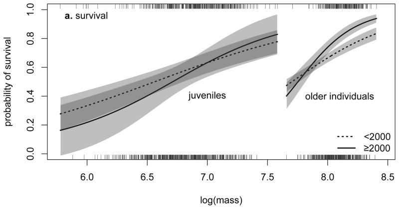
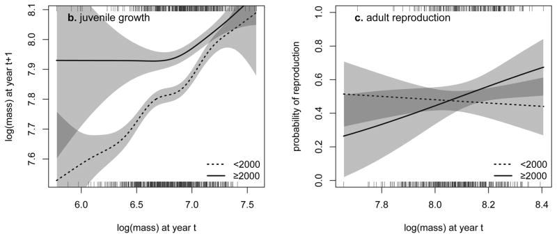
Our next objective was to understand why these joint changes have been observed. We used mark-recapture methods²⁶ and generalized linear and additive models²⁷ to identify the most parsimonious functions describing associations between body mass and demographic (survival, reproduction probability and litter size) and trait transition (growth and offspring body mass) rates. We also tested for the effects of age-class and study period on these rates. Body mass had a significant positive influence on most rates in both periods (Figs. S4–S7). Moreover, the form of some of the body mass-rate functions has also changed over time. Heavier marmots, particularly adults, survived better in later years (Fig. 2A). Both mean juvenile growth (from first to second August of life) and the dependence of growth on mass have increased in later years (Fig 2B); the resulting increase in growth was much greater among smaller juveniles. In addition, heavier females had a higher chance of reproducing in later years (Fig. 2C).

Figure 2.

The relationship between body mass and (A) survival, (B) juvenile growth, and (C) adult reproduction for <2000 and ≥2000 years. Shaded areas indicate the 95% confidence intervals, and rugs below and above the graph represent the distribution of the body mass data for <2000 and ≥2000 years, respectively.

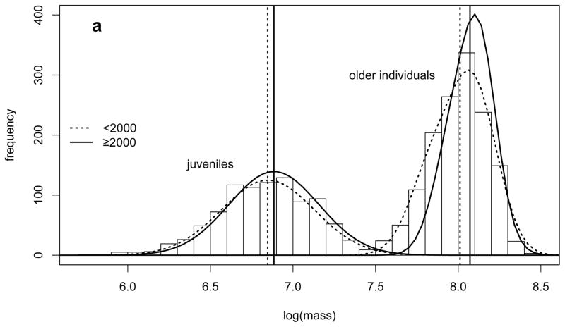
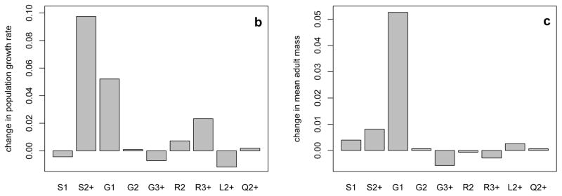
To understand the population dynamic and phenotypic consequences of these changes, we used a recently developed method, an integral projection model (IPM)^28,29, which projects the distribution of a continuous trait based on demographic and trait transition functions. Using the fitted functions relating body mass to each rate, we parameterized two IPMs, one for the pre-2000 period and one for post-2000. Eigen-analysis of the two IPMs captured the observed change in the dynamics: the asymptotic population growth increased from an approximately stable λ = 1.02 in the earlier period to a rapidly increasing λ = 1.18 in the later period (Fig. 1C). The stable mass distributions for each of the periods captured the observed increase in body mass in both juveniles (+38.2 g, 4.2%) and older age classes (+166.7 g, 5.8%) (Fig. 3A). To identify which demographic or trait transition function had contributed most to the observed increase in population growth rate, we performed a retrospective perturbation analysis of the two IPMs. The observed increase in population growth rate was predominantly due to changes in the adult survival and juvenile growth functions (Fig. 3B).

Figure 3.

(A) Stable August log-body mass distributions (lines) for juveniles and older individuals for <2000 and ≥2000 years. Vertical lines show the mean body masses. Bars indicate the actual observed distribution over the entire study period. Retrospective perturbation analysis of the integral projection model gives the relative contribution of each function to (B) population growth and to (C) change in mean adult body mass from <2000 to ≥2000 period (S: survival, G: growth, R: reproduction probability, L: litter size, Q: offspring mass, subscripts indicate the age classes).

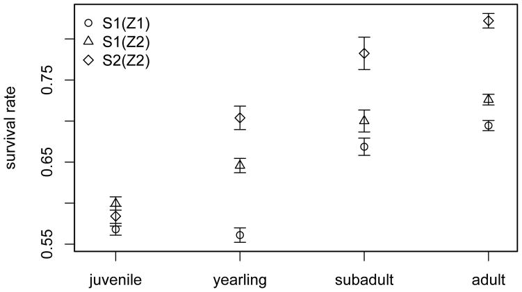
The increase in mean adult survival was the key demographic factor underlying the observed shift in population dynamics between the two periods. It could have been caused by two non-mutually exclusive processes: (1) a change in the relationship between August mass and survival, and (2) a change in mean August mass in each age class. To understand the relative contributions of these two processes, we estimated three mean survival rates for each age-class using (1) the earlier period’s survival curve and trait distribution, S₁(Z₁), (2) the earlier period’s survival curve and the later period’s trait distribution, S₁(Z₂), and finally (3) the later period’s survival curve and trait distribution, S₂(Z₂). The difference between (2) and (1) versus the difference between (3) and (2) indicates the contributions of the change in mean mass versus the change in survival curve. The juvenile survival did not change substantially, yet the observed small increase was caused by a change in the mass distribution. For older marmots, both processes had comparable contributions to the increase in survival (Fig. 4). The change in the mass distribution contributed slightly more to the increase in yearling survival, whereas the change in the survival curve contributed more to the increase in subadult and adult survival. As the increase in the survival of older individuals is the prominent cause of the observed population increase, both the faster growth of marmots and the change in the relationship between survival and August mass must have played an important role in the observed shift in population dynamics.

Figure 4.

The relative contributions of the change in mean August mass (Z1 to Z2) and the change in survival curve (S1 to S2) to the increase in mean survival in each age class from <2000 to ≥2000 years. The proximity of the triangle [S1(Z2)] to the circle [S1(Z1)] versus to the diamond [S2(Z2)] indicates the contributions of the change in mean mass versus the change in survival curve. Confidence intervals indicate the process variation estimated using the particular mass distribution and survival function.

Finally, to understand the processes underlying the observed phenotypic change, we decomposed the change in mean body mass ΔZ̄ into contributions from selection and other processes using the recently developed age-structured Price equation²¹ (Fig. S8A). The mean annual growth of juveniles has increased from 1523.7 (SE=45.1) g/year for pre-2000 to 1847.4 (78.1) g/year for post-2000 years (p < 0.01). This faster growth from first to second August of life has resulted in higher mean body masses in the older age classes as also demonstrated by the retrospective perturbation analysis of the IPMs (Fig. 3C). The temporal change in mean body mass for the whole population over the 33 years was predominantly explained by changes in the mean growth rate contributions (52%), with selection-related terms contributing only 3% (Fig. S8B), suggesting that the change in body mass is not the result of a change in selection operating on the trait.

How can we interpret these results? The population-level response to environmental change was mediated to a large extent through environmental influences on body mass. The increase in the length of the growing season has altered the phenology; marmots are now born earlier than they once were and they have more time to grow until the next hibernation. This increase in juvenile growth has caused an increase in body mass in all age-classes. Yet, most of this change was an ecological (plastic) rather than an evolutionary response to environmental change as also seen in Soay sheep on St Kilda²². This increase in body mass and the length of the growing season has additionally altered the functional dependence of vital rates on body mass. Heavier marmots now survive and reproduce better than they once did, and this has led to a rapid increase in population size in recent years.

A simultaneous response to environmental change in phenology, phenotypic traits and population dynamics appears to be common-place in nature². We have demonstrated, for the first time, how such joint dynamics can be investigated, and have shown how changes in phenotypic traits and population dynamics can be intimately linked. If we are to understand the biological consequences of environmental change it will prove necessary to gain further insight into these linkages. Despite this, we do not completely understand why the body mass - demography associations changed as dramatically as we observe. This means predicting future change will prove more challenging than characterising past change. We suspect that the observed increase in marmot survival is likely to be a short-term response to the lengthening growing season. Longer-term consequences may hinge on whether long, dry summers become more frequent, as this would decrease growth rates and increase mortality rates. Characterising observed interactions between environment, phenotypic traits and demography is challenging; accurately predicting how they may change in the future will almost certainly require a mechanistic understanding of how environmental change impacts resource availability as well as individual energy budgets³⁰.

Methods

The study system

The yellow-bellied marmot is a large, diurnal, burrow-dwelling rodent, occupying montane regions of western North America ^25,31. The species hibernates from September or October to April or May, during which time individuals lose approximately 40% of their body mass²⁵. The need to mobilize energy for reproduction and then prepare for hibernation in a short time period accounts for the energy conservative physiology of this species^32,33. The critical factor determining winter survival and subsequent reproductive success is the amount of fat accumulated prior to hibernation^34,35. Upon emergence all age classes start gaining mass at the rate of about 12 to 14 g/day. The annual cycle is a major constraint on population dynamics. The need to satisfy the energy requirements for hibernation limits reproduction to a single annual event occurring immediately after emergence. The short active season combined with large body size delays reproductive maturity until two years of age³⁶.

This study was conducted in the Upper East River Valley near the Rocky Mountain Biological Laboratory, Gothic, Colorado (38° 57′ N, 106° 59′ W). Data were collected from 17 distinct sites within the study area^37,38. From 1962 to 2008, yellow-bellied marmots were live-trapped at each site throughout the active season (May–September) and individually marked using numbered ear tags³⁹. Animal identification number, sex, mass and reproductive condition were recorded at each capture. Ages for females that were captured as juveniles were known, whereas ages for other females were estimated based on body mass (≤ 2 kg = yearling, > 2 kg = adult)²⁴. In this study, we omitted the <1976 years due to lower sampling effort.

Survival and reproduction are affected by the length of the active season, which varies from year to year as a consequence of variation in the onset and/or termination of snow cover^40,41. The length of the growing season also varies among marmot sites over a distance of 4.8 km in the Upper East River Valley where the greatest difference in elevation between colonies is 165 m. The biology of yellow-bellied marmots in Colorado is described in further detail elsewhere ^25,39.

Estimation of August 1^st body mass

Marmot life-history is tightly related to the circannual rhythm ²⁵. As marmots loose ca. 40% of their body mass during hibernation²⁵ and females give birth in late-May, the mean body mass changes substantially over the active season and among age classes. Furthermore, the study area includes multiple sites with different elevations and aspects and the environmental conditions vary among years, causing variation in mean body mass among sites and years at a given date. In this study, we focus on the estimated August 1^st body mass as it provides the best trade-off between data availability and biological significance. The trapping data until mid-August is sufficient to provide a good estimate of body mass, from which point on the data becomes sparse in most years (Fig. S2). August mass is biologically significant for several reasons: (1) It is beyond the influence of the previous hibernation, particularly for non-reproductive stages. (2) Marmots are weaned no later than mid-July and there is no reproductive activity until the following spring. Therefore, August 1^st mass is not confounded by pregnancy. (3) As the plant mass growth peaks in mid-July ^33,42, growth plateaus in early August for non-reproductive adults, mid-August for young and late August for reproductive females ^25,43,44. Therefore, it covers most of the critical period for individual growth.

The body mass data were collected from each individual at multiple captures throughout the active season. Individuals were captured at an average of 3.12 times in a given year with a maximum of 7.45 captures in 2003. We grouped individuals into four age classes: juvenile (a=1: year 0–1), yearling (a=2: year 1–2), subadult (a=3: year 2–3), and adult (a=4: year >3). To estimate the August 1^st body mass for each individual/year, we constructed a general linear mixed model including the fixed effect of day-of-year on body mass, and the random effects of year, site and individual ID. Models were fitted with the lme4 package ⁴⁵. A separate model was fitted to each age class and random deviations were incorporated in both the intercept and the (linear) day-of-year term for all three random effects. Because it includes multiple age classes (≥3 yrs old), the adult model also incorporates a random “observation age” term (nested within individual) to accommodate individual level variation in size among successive observation years. We did not attempt to determine whether specific variance components were significantly different from zero. This is unnecessary when the goal of modelling is prediction; negligible sources of variation are simply estimated to be near zero and thus contribute little to predicted values. For all four age classes, we compared a set of nested models for the fixed effects structure which incorporated up to third order polynomial terms for day-of-year. The set of models constructed for adults also considered models with a fixed effect of age and the interaction of age with day-of-year. Fixed effect structures were compared using likelihood ratio tests ⁴⁶. Some caution is required when applying likelihood ratio tests to examine the significance of fixed effects as these are known to be anticonservative. Fortunately all of the results we report were highly significant.

The most parsimonious models included second order polynomial terms for day-of-year in juveniles and yearlings, and only the linear effect in subadults and adults (Fig. S2). The most parsimonious adult model also included an age effect but not the interaction term with day-of-year. For example, in juveniles and yearlings the expected mass of an individual at observation is given by,

$$E\left[{\mu }_i\right]=\left({\beta }_0+u_{fm(i),0}+v_{yr(i),0}+w_{st(i),0}\right)+\left({\beta }_1+u_{fm(i),1}+v_{yr(i),1}+w_{st(i),1}\right)D+{\beta }_2{D}^2$$

where D is the day-of-year; u, v and w reference the random female, year, and site effects, respectively; β₁ and β₂ are the linear and quadratic fixed effect terms for day-of-year, respectively; and β₀ is the global intercept. In the random terms, the first subscript (e.g. yr(i)) can be viewed as a mapping function referencing the appropriate random effect level for observation i, and the second subscript references the random intercept or slope term as appropriate. Using the fitted models, we predicted the August 1^st (214^th day-of-year) mass for each individual conditional on the predicted random effects given by the BLUPs (i.e. the Best Linear Unbiased Predictors). We used these estimated August 1^st masses for the rest of the analyses.

Relationship between body mass and demographic and trait transition rates

To understand the link between phenotypic dynamics and population dynamics, we examined the relationship between body mass and each of the five demographic and trait transition rates using the long-term individual-based data. The demographic rates are (1) the survival from one year to the next (0 or 1), (2) reproducing the following year conditional on survival (0 or 1), and (3) litter size conditional on reproduction (≥1), whereas the trait transition rates are (4) the ontogenic growth from one August to the next and (5) the average August 1^st body mass of the offspring (i.e., juvenile) produced to the next year. It is important to note that most of the juvenile growth (from its first to second August of life) occurs after individuals emerge from their first hibernation as yearlings; similarly, most of the yearling growth (from its second to third August of life) occurs after individuals emerge from their second hibernation as subadults.

For the analysis of survival rates, we used a multistate mark-recapture model²⁶ implemented using Program MARK⁴⁷ with the RMark interface⁴⁸ where we tested for the effect of body mass (as a time-varying individual covariate) on stage-specific survival rates. For the rest of the rates, the functions were characterized using generalized linear and additive models, GAMs²⁷, as the associations between quantitative traits and demographic rates could be non-linear^49,50. For each rate, the number of demographic classes were determined by comparing models with different stage structures using Akaike’s information criterion⁵¹.

We next tested for linear, non-linear, and two-way interaction effects of the current August body mass, age-class and study period. All rates, except for litter size and offspring mass, showed significant changes from the earlier to the later period (Table S1), and body mass had a significant influence on all rates during both periods. Moreover, the relationship between body mass and some of the demographic and trait transition rates significantly differed between the two periods (Figures S4–S7). The general models describing the demographic and trait transition rates are summarized in Table S1.

Construction of the integral projection models

The above analysis of demographic and trait transition rates showed that individual fates are influenced by their body mass and age class. To accommodate both factors in an efficient manner, we construct a stage- and mass-structured integral projection model (IPM). General IPMs project the distribution of discrete and continuous trait-structured population in discrete time. Their main advantage is that they allow parsimonious modelling of changes in both the phenotypic distribution and population growth rate based on easily estimated demographic and trait transition functions²⁸. Theory for general IPMs in a constant environment and an example application of an age- and size-structured model can be found in Ellner and Rees²⁹ and Childs et al.⁵², respectively. Using the most parsimonious functions relating body mass to each demographic and trait transition rate, we parameterized two IPMs, one for earlier (<2000) and one for later (≥2000) years.

The two main elements of an IPM are the projected trait distributions for each stage class and the projection kernel components. Our IPM tracks the distribution of body mass in juvenile (a = 1), yearling (a = 2), subadult (a = 3), and adult (a = 4) stages. For a general stage class a, the number of individuals in the mass range [x,x + dx]at time t is denoted by n_a(x,t). The dynamics of n_a(x,t) are governed by a set of coupled integral equations

$$\begin{gathered} n_1(y,t+1)=\sum _{a=2}^4\underset{\mathrm{\Omega }}{\int }{F}_a(y,x)n_a(x,t)dx \\ {n}_{a+1}(y,t+1)=\underset{\mathrm{\Omega }}{\int }{P}_a(y,x)n_a(x,t)dx(\text{for}a=1,2,3) \\ {n}_4(y,t+1)=\underset{\mathrm{\Omega }}{\int }{P}_3(y,x)n_3(x,t)dx+\underset{\mathrm{\Omega }}{\int }{P}_4(y,x)n_4(x,t)dx \end{gathered}$$

where Ω is a closed interval characterising the mass domain, F_a(y,x) are recruitment kernels that determine the contribution of juvenile, subadult and adult stages to the next generation, and P_a(y,x) are survival-growth kernels that determine the transitions among (or in the case of adults, within) the four life stages.

These kernels are implied directly by the statistical analysis of the data; the necessary functions are already parameterized for the two periods and summarized in Table S1. The survival-growth kernel for individuals of age a is given by

$$P_a(y,x)=S_a(x)G_a^{\prime }(y,x)$$

An individual that remains in the population must survive over winter and grow. The prime notation in the growth kernel is present to highlight that this function is not the same object as the corresponding demographic growth model in Table S1, but rather it is the conditional distribution of y given x (which is easily derived from the demographic growth model). The recruitment kernels are given by

$$F_a(y,x)=S_a(x)R_a(x)L_a(x)Q_a^{\prime }(y,x)$$

Reading from left to right, we see that in order to contribute a juvenile to the population in the following summer, a current individual with mass x must survive over winter and successfully reproduce in the following summer, giving rise to female recruits with mass y, the number and size of which depends on the reproducing adults size. The prime notation present in the identifier of the offspring mass kernel serves the same purpose as that in the adult growth kernel above. The model only accounts for females, thus L_a(x) is the number of female offspring. Having specified the survival-growth and fecundity kernels, the model is now complete.

Sequential iteration of the IPM entails repeated numerical integration. To achieve this, we used a simple method called the midpoint rule. This method constructs a discrete approximation of the IPM on a set of ‘mesh points’ and then uses matrix multiplication to iterate the model. Similarly, computation of the asymptotic growth rate and stable age × mass distribution is achieved by following the common procedures for a matrix projection model⁵³. A detailed explanation of the midpoint rule is given in Ellner and Rees²⁹. The accuracy of the method depends on the size of the mesh; increasing this improves the numerical accuracy of the approximation. We chose to divide the body mass interval into 50 mass classes, as this ensures the population growth rate calculations are accurate to at least 3 decimal places.

Retrospective perturbation analysis of the IPM

To identify which one of the nine demographic and trait transition functions (Table S1) had contributed the most to the observed increase in λ from earlier to later period, we performed a retrospective perturbation analysis of the two IPMs. We, first, created a design matrix with 9 columns representing all the functions (Table S1) and 2⁹ rows representing all possible combinations of change among these 9 functions. The entries of the design matrix are 0 or 1, indicating if the function is parameterized using <2000 or ≥2000 data, respectively. Next, for each combination, we created an IPM and estimated the corresponding λ. Using the dummy coding for each of the nine functions as binary explanatory variables and λ as the response variable, we tested for the main effects of and two-way interactions between each of the nine functions. The main-effects model explained a substantial amount of the variation in λ (R² = 98.7%); therefore, we ignored the two-way interactions. The resulting regression effect sizes denote the change in λ contributed by the change in each of the nine demographic and trait transition components. Similarly, we estimated the contribution of each functional change to the mean adult mass by estimating a mean adult mass from the stable size distribution (right eigenvector) for each combination and applying the same methodology outlined above.

The age-structured Price equation

Finally, to understand the processes underlying the observed phenotypic change, we decomposed the change in mean body mass ΔZ̄ into contributions from selection and other processes using the age-structured Price equation^21,22. The exact change in mean value of a trait over a time step ΔZ̄(t) = Z̄(t + 1) − Z̄(t) is decomposed into seven contributions. The mathematical details are provided in Coulson and Tuljapurkar²¹ and Ozgul et al.²². Here, we provide further details on the interpretation of terms in Figure S8A. The DCs term describes change in Z̄ resulting from changes in demographic composition due to ageing, whereas DCr term describes the change in Z̄ resulting from the addition of new individuals due to birth. The VS term is the viability selection differential on Z across all individuals; it describe how selective removal of individuals through mortality alters Z̄. The contribution to Z̄ from age-specific trait development (i.e., growth or reversion) among individuals that survive is captured in the GR term. The FS term is the reproductive selection differential, which describes how Z̄ differs between parents and the unselected population. The OMD term represents the contribution of differences between offspring and parental trait values to Z̄. The ODC term describes the contribution from any covariance between OMD and number of offspring produced by each individual. Each of these terms is weighted by demographic sensitivities, which describes how survival or reproduction in an age class contributes to population growth.

All analyses in this study were performed using the statistical and programming package, R⁵⁴.

References

- 1.Walther G, et al. Ecological responses to recent climate change. Nature. 2002;416:389–395. doi: 10.1038/416389a. [DOI] [PubMed] [Google Scholar]
- 2.Parmesan C. Ecological and evolutionary responses to recent climate change. Annual Review of Ecology Evolution and Systematics. 2006;37:637–669. [Google Scholar]
- 3.Stenseth N, Mysterud A. Climate, changing phenology, and other life history traits: Nonlinearity and matchñmismatch to the environment. Proceedings of the National Academy of Sciences. 2002;99:13379. doi: 10.1073/pnas.212519399. [DOI] [PMC free article] [PubMed] [Google Scholar]
- 4.Coulson T, Benton TG, Lundberg P, Dall SRX, Kendall BE. Putting evolutionary biology back in the ecological theatre: a demographic framework mapping genes to communities. Evolutionary Ecology Research. 2006;8:1155–1171. [Google Scholar]
- 5.Chevin LM, Lande R, Mace GM. Adaptation, plasticity and extinction in a changing environment: Towards a predictive theory. PLoS Biology. doi: 10.1371/journal.pbio.1000357. (submitted) [DOI] [PMC free article] [PubMed] [Google Scholar]
- 6.IPCC. The Physical Science Basis: Contribution of Working Group I to the Fourth Assessment Report of the IPCC. Cambridge; 2007. [Google Scholar]
- 7.Karl T, Trenberth K. Modern global climate change. Science. 2003;302:1719. doi: 10.1126/science.1090228. [DOI] [PubMed] [Google Scholar]
- 8.Inouye DW, Barr B, Armitage KB, Inouye BD. Climate change is affecting altitudinal migrants and hibernating species. Proceedings of the National Academy of Sciences. 2000;97:1630–1633. doi: 10.1073/pnas.97.4.1630. [DOI] [PMC free article] [PubMed] [Google Scholar]
- 9.Thomas C, Lennon J. Birds extend their ranges northwards. Nature. 1999;399:213. [Google Scholar]
- 10.Pounds J, et al. Widespread amphibian extinctions from epidemic disease driven by global warming. Nature. 2006;439:161–167. doi: 10.1038/nature04246. [DOI] [PubMed] [Google Scholar]
- 11.Jenouvrier S, et al. Demographic models and IPCC climate projections predict the decline of an emperor penguin population. Proceedings of the National Academy of Sciences. 2009;106:1844–1847. doi: 10.1073/pnas.0806638106. [DOI] [PMC free article] [PubMed] [Google Scholar]
- 12.Fisher RA. The genetical theory of natural selection. 1958 [Google Scholar]
- 13.Bradshaw W, Holzapfel C. Evolutionary response to rapid climate change. Science. 2006;312:1477–1478. doi: 10.1126/science.1127000. [DOI] [PubMed] [Google Scholar]
- 14.Via S, et al. Adaptive phenotypic plasticity: consensus and controversy. Trends in Ecology & Evolution. 1995;10:212–217. doi: 10.1016/s0169-5347(00)89061-8. [DOI] [PubMed] [Google Scholar]
- 15.Reale D, McAdam AG, Boutin S, Berteaux D. Genetic and plastic responses of a northern mammal to climate change. Proceedings of the Royal Society of London Series B-Biological Sciences. 2003;270:591–596. doi: 10.1098/rspb.2002.2224. [DOI] [PMC free article] [PubMed] [Google Scholar]
- 16.Lande R. Natural selection and random genetic drift in phenotypic evolution. Evolution. 1976;30:314–334. doi: 10.1111/j.1558-5646.1976.tb00911.x. [DOI] [PubMed] [Google Scholar]
- 17.Berthold P, Helbig AJ, Mohr G, Querner U. Rapid microevolution of migratory behavior in a wild bird species. Nature. 1992;360:668–670. [Google Scholar]
- 18.Gienapp P, Teplitsky C, Alho JS, Mills JA, Merila J. Climate change and evolution: disentangling environmental and genetic responses. Molecular Ecology. 2008;17:167–178. doi: 10.1111/j.1365-294X.2007.03413.x. [DOI] [PubMed] [Google Scholar]
- 19.Tuljapurkar S, Caswell H. Structured-population models in marine, terrestrial, and freshwater systems. Chapman & Hall; 1997. [Google Scholar]
- 20.Saether B, et al. Population dynamical consequences of climate change for a small temperate songbird. Science. 2000;287:854. doi: 10.1126/science.287.5454.854. [DOI] [PubMed] [Google Scholar]
- 21.Coulson T, Tuljapurkar S. The dynamics of a quantitative trait in an age-structured population living in a variable environment. American Naturalist. 2008;172 doi: 10.1086/591693. [DOI] [PMC free article] [PubMed] [Google Scholar]
- 22.Ozgul A, et al. The dynamics of phenotypic change and the shrinking sheep of St. Kilda. Science. 2009;325:464–467. doi: 10.1126/science.1173668. [DOI] [PMC free article] [PubMed] [Google Scholar]
- 23.Pelletier F, Clutton-Brock T, Pemberton J, Tuljapurkar S, Coulson T. The evolutionary demography of ecological change: Linking trait variation and population growth. Science. 2007;315:1571–1574. doi: 10.1126/science.1139024. [DOI] [PubMed] [Google Scholar]
- 24.Armitage KB, Downhower JF, Svendsen GE. Seasonal changes in weights of marmots. American Midland Naturalist. 1976;96:36–51. [Google Scholar]
- 25.Armitage KB. In: Wild Mammals of North America: Biology, Management, and Conservation. 2. Feldhamer GA, Thompson BC, Chapman JA, editors. Johns Hopkins University Press; 2003. pp. 188–210. [Google Scholar]
- 26.Brownie C, Hines JE, Nichols JD, Pollock KH, Hestbeck JB. Capture-recapture studies for multiple strata including non-Markovian transitions. Biometrics. 1993;49:1173–1187. [Google Scholar]
- 27.Wood SN. Generalized Additive Models: An Introduction with R. Chapman & Hall; 2006. [Google Scholar]
- 28.Easterling MR, Ellner SP, Dixon PM. Size-specific sensitivity: Applying a new structured population model. Ecology. 2000;81:694–708. [Google Scholar]
- 29.Ellner SP, Rees M. Integral projection models for species with complex demography. American Naturalist. 2006;167:410–428. doi: 10.1086/499438. [DOI] [PubMed] [Google Scholar]
- 30.Humphries M, Umbanhowar J, McCann K. Bioenergetic prediction of climate change impacts on northern mammals. Integrative and Comparative Biology. 2004;44:152. doi: 10.1093/icb/44.2.152. [DOI] [PubMed] [Google Scholar]
- 31.Frase BA, Hoffmann RS. Marmota flaviventris. Mammalian Species. 1980;135:1–8. [Google Scholar]
- 32.Armitage KB, Melcher JC, Ward JM. Oxygen consumption and body temperature in yellow-bellied marmot populations from montane-mesic and lowland-xeric environments. Journal of Comparative Physiology B. 1990;160:491–502. [Google Scholar]
- 33.Kilgore DL, Armitage KB. Energetics of yellow-bellied marmot populations. Ecology. 1978;59:78–88. [Google Scholar]
- 34.Andersen D, Armitage K, Hoffmann R. Socioecology of marmots: female reproductive strategies. Ecology. 1976;57:552–560. [Google Scholar]
- 35.Melcher J, Armitage K, Porter W. Energy allocation by yellow-bellied marmots. Physiological Zoology. 1989;62:429–448. [Google Scholar]
- 36.Armitage KB. Sociality as a life-history tactic of ground-squirrels. Oecologia. 1981;48:36–49. doi: 10.1007/BF00346986. [DOI] [PubMed] [Google Scholar]
- 37.Armitage KB. Reproductive strategies of yellow-bellied marmots: Energy conservation and differences between the sexes. J Mammal. 1998;79:385–393. [Google Scholar]
- 38.Ozgul A, Oli MK, Armitage KB, Blumstein DT, Van Vuren DH. Influence of local demography on asymptotic and transient dynamics of a yellow-bellied marmot metapopulation. American Naturalist. 2009;173:517–530. doi: 10.1086/597225. [DOI] [PubMed] [Google Scholar]
- 39.Armitage KB. Social and population dynamics of yellow-bellied marmots - results from long-term research. Annual Review of Ecology and Systematics. 1991;22:379–407. [Google Scholar]
- 40.Armitage KB, Downhower JF. Demography of yellow-bellied marmot populations. Ecology. 1974;55:1233–1245. [Google Scholar]
- 41.Schwartz OA, Armitage KB, Van Vuren D. A 32-year demography of yellow-bellied marmots (Marmota flaviventris) J Zool. 1998;246:337–346. [Google Scholar]
- 42.Frase BA, Armitage KB. Yellow-bellied marmots are generalist herbivores. Ethology Ecology & Evolution. 1989;1:353–366. [Google Scholar]
- 43.Woods BC, Armitage KB. Effect of food supplementation on juvenile growth and survival in Marmota flaviventris. J Mammal. 2003;84:903–914. [Google Scholar]
- 44.Armitage KB. In: Biodiversity in marmots. Le Berre M, Ramousse R, Le Guelte L, editors. International Marmot Network; 1996. pp. 223–226. [Google Scholar]
- 45.R package version 0.999375–32. 2009. lme4: Linear mixed-effects models using S4 classes v. [Google Scholar]
- 46.Pinheiro JC, Bates DM. Mixed Effects Models in S and S-PLUS. Springer-Verlag; 2000. [Google Scholar]
- 47.White GC, Burnham KP. Program MARK: survival estimation from populations of marked animals. Bird Stud. 1999;46:120–139. [Google Scholar]
- 48.Laake J, Rexstad E. Cooch E, White GC, editors. Program MARK: a gentle introduction. 2007 http://www.phidot.org/software/mark/docs/book/
- 49.Schluter D. Estimating the form of natural selection on a quantitative trait. Evolution. 1988;42:849–861. doi: 10.1111/j.1558-5646.1988.tb02507.x. [DOI] [PubMed] [Google Scholar]
- 50.Kingsolver JG, et al. The strength of phenotypic selection in natural populations. American Naturalist. 2001;157:245–261. doi: 10.1086/319193. [DOI] [PubMed] [Google Scholar]
- 51.Burnham KP, Anderson DR. Model selection and inference: a practical information-theoretic approach. 2. Springer-Verlag; 2002. [Google Scholar]
- 52.Childs D, Rees M, Rose K, Grubb P, Ellner S. Evolution of complex flowering strategies: an age-and size-structured integral projection model. Proceedings of the Royal Society B: Biological Sciences. 2003;270:1829. doi: 10.1098/rspb.2003.2399. [DOI] [PMC free article] [PubMed] [Google Scholar]
- 53.Caswell H. Matrix population models: construction, analysis, and interpretation. Sinauer; 2001. [Google Scholar]
- 54.R: A language and environment for statistical computing. R Foundation for Statistical Computing; Vienna, Austria: 2008. ( http://www.R-project.org) [Google Scholar]
Associated Data
This section collects any data citations, data availability statements, or supplementary materials included in this article.