A Bayesian Screening Approach for Hepatocellular Carcinoma using Multiple Longitudinal Biomarkers

Summary

Advanced hepatocellular carcinoma (HCC) has limited treatment options and poor survival, therefore early detection is critical to improving the survival of patients with HCC. Current guidelines for high-risk patients include ultrasound screenings every 6 months, but ultrasounds are operator dependent and not sensitive for early HCC. Serum α-Fetoprotein (AFP) is a widely used diagnostic biomarker but it has limited sensitivity and is not elevated in all HCC cases so we incorporate a second blood-based biomarker, des-γ carboxy-prothrombin (DCP), that has shown potential as a screening marker for HCC. The data from the Hepatitis C Antiviral Long-term Treatment against Cirrhosis (HALT-C) Trial is a valuable source of data to study biomarker screening for HCC. We assume the trajectories of AFP and DCP follow a joint hierarchical mixture model with random changepoints that allows for distinct changepoint times and subsequent trajectories of each biomarker. The changepoint indicators are jointly modeled with a Markov Random Field distribution to help detect borderline changepoints. Markov chain Monte Carlo methods are used to calculate posterior distributions, which are used in risk calculations among future patients and determine whether a patient has a positive screen. The screening algorithm was compared to alternatives in simulations studies under a range of possible scenarios and in the HALT-C Trial using cross-validation.

1. Introduction

In the United States, the incidence of hepatocellular carcinoma (HCC) has tripled over the last two decades, while the five-year survival of patients with HCC has remained largely unchanged at <12% (El-Serag, 2011). Patients with early stage HCC have multiple treatment options and the 5-year survival for treated patients exceeds 60% (Bruix and Sherman, 2005). Five-year survival for HCC cases that are diagnosed at a later (symptomatic) stage is between 0–10%. Early detection of HCC through surveillance is critical to reducing mortality.

The target population for HCC surveillance are those patients with cirrhosis, since 80–90% of HCC cases occur in patients with cirrhosis. Six-month ultrasonography is recommended (Bruix and Sherman, 2011); however, there is disagreement over the benefit of surveillance. In the United States, the majority of surveillance ultrasounds are performed at local hospitals with variable quality because ultrasonography is operator dependent, not sensitive in detecting early lesions and difficult to perform in obese patients. Serum α-Fetoprotein (AFP) is a diagnostic HCC biomarker widely used to complement ultrasonography. The reported sensitivity for AFP varies between 41–100% and specificity between 70–95% in both diagnostic and screening settings and across a range of study designs (Gebo et al., 2002). Des-γ carboxy-prothrombin (DCP) has shown potential as a complementary screening biomarker for HCC (Marrero et al., 2009). In many cancers, including HCC, a single biomarker is unlikely to identify all disease subtypes and screening with multiple biomarkers is necessary to produce a highly sensitive test. It is important to differentiate between risk models that predict the future development of disease and the focus of our paper— screening approaches to detect current asymptomatic disease.

To date, most studies evaluating AFP and DCP have compared current biomarker levels to a fixed threshold (Gebo et al., 2002; Marrero et al., 2009; Lok et al., 2010) but the longitudinal trajectory of biomarkers contains valuable information. In ovarian cancer, Drescher et al. (2013) demonstrated higher sensitivity of a univariate parametric empirical Bayes (PEB) screening algorithm— first proposed by McIntosh and Urban (2003)— applied to cancer antigen 125 (CA 125) compared to the standard threshold approach. Skates et al. (2001) proposed a fully Bayesian screening algorithm that also improved sensitivity of CA 125 for ovarian cancer. In HCC screening, Lee et al. (2013) found evidence that trends in AFP have prognostic value but their approach required at least five prior measurements. Tayob et al. (2016) implemented a univariate PEB screening algorithm for AFP that produced significant gains in sensitivity over the standard threshold approach.

In the Skates et al. (2001) fully Bayesian screening algorithm for a single longitudinal biomarker, the decision rule is based on the posterior risk of disease at the current screen, given all the screening values to date. An estimate of the posterior risk requires specifying a model for the biomarker trajectory. Skates et al. (2001) assume that in patients with no cancer the biomarker trajectory is stable but after the onset of cancer (early in the disease course) we may or may not observe a steady increase of the biomarker level and this longitudinal trajectory is modeled via a hierarchical change-point and mixture model. Norris et al. (2009) propose a longitudinal model for a single biomarker where in the absence of disease the biomarker trajectory is stable and in the presence of disease all patients will have an increase in their biomarker levels but there is a lag between disease onset and the changepoint time. The two models make different assumptions about the underlying disease mechanisms and the approach of Skates et al. (2001) is more in line with our application.

In addition to providing usable R codes to implement the methodology of Skates et al. (2001), which are currently not available, we extend their fully Bayesian univariate screening algorithm to screening with multiple correlated longitudinal biomarkers. This extension is not trivial. Our proposed joint model for the multiple biomarker trajectories assumes that each biomarker may or may not exhibit a characteristic change in their trajectory after the onset of cancer, but neither the existence of a changepoint, the timing of said changepoint nor the rate of change is assumed to be uniform across the biomarkers.

We propose a robust computationally efficient screening algorithm that exploits all the available biomarker information. Patients undergoing screening often miss scheduled visits and rarely follow the recommended surveillance interval. We may also have only a subset of the biomarkers are measured at any particular visit (e.g. a screening algorithm with standard serum markers measured more frequently and expensive assays less frequently). Our proposed methodology can accommodate both unevenly spaced screening visits and “missing data”.

An ideal HCC biomarker would change trajectory early in the disease course. A positive screen would trigger further imaging with more sensitive modalities, such as magnetic resonance imaging (MRI) or computed tomography (CT), and increase the likelihood of detecting early stage cancer where patients have multiple viable treatment options and simultaneously maintain affordable costs. The potential accuracy of a screening algorithm must be fully evaluated before being used in a prospective trial. The Hepatitis C Antiviral Long-term Treatment against Cirrhosis (HALT-C) Trial has provided valuable biomarker data to study HCC screening (Lok et al., 2010; Sterling et al., 2012; Lee et al., 2013; Tayob et al., 2016). The multi-center study had extensive follow-up in patients resulting in a rich source of data to better understand screening approaches with multiple longitudinal biomarkers in cirrhosis patients. We begin by describing the HALT-C trial data in Section 2. In Section 3 we outline each element of the proposed screening approach, including the joint model for multiple longitudinal biomarkers and the computational procedure used to obtain the posterior distributions needed in the posterior risk calculations. The operational characteristics of the screening algorithm are studied in simulations (Section 4). In Section 5 we present the results from applying the screening approach to the data from the HALT-C Trial. A discussion follows in Section 6.

2. HALT-C Trial

The HALT-C Trial evaluated an interferon-based therapy that aimed to prevent fibrosis progression and other clinical outcomes in patients with chronic hepatitis C virus (HCV) infection and either bridging fibrosis or cirrhosis. Patients underwent extensive follow-up and were monitored for the development of HCC. Visits were scheduled every three months for the first 42 months post-randomization and every six months thereafter. At each visit, patients were evaluated clinically and had local laboratory tests, including AFP. DCP was measured at a central laboratory in an ancillary study that used stored samples collected during the first 42 months post-randomization. Patients had an ultrasound of the liver at 6, 18, 30 and 42 months post-randomization and every six months thereafter. Patients with new lesions on ultrasound or elevated AFP were further evaluated with CT or MRI. HCC diagnosis was based on histology and in its absence, by imaging with or without AFP. We evaluated HCC screening in all patients, regardless of assigned treatment, since there was no evidence the incidence of HCC differed between the two treatment groups (Lok et al., 2011).

HCV-cirrhosis patients are at high-risk and recommended for HCC surveillance. The analysis cohort includes 48 confirmed HCC cases and 361 control patients with no HCC during a median follow-up period of 78 months (range 15–109 months) (Web Figure 1).

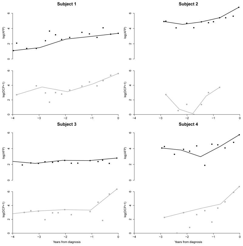
In Figure 1 we plot the trajectory of AFP and DCP prior to HCC diagnosis in 4 of the 48 HCC cases. Subject 1 had increasing AFP and DCP but the changepoint for AFP was less clearly defined compared to DCP. By jointly modeling the changepoints, we aim to borrow information across the markers and identify changepoints that are more subtle. In Subject 2, we observed a clear changepoint for AFP but the large variability in DCP makes it difficult to identify the changepoint without borrowing information from the AFP trajectory. Subject 3’s AFP levels did not increase but they have a clearly defined changepoint in DCP one-year prior to clinical diagnosis. This HCC case would not be detected with AFP screening alone. Subject 4 has clearly identifiable changepoints for both AFP and DCP but the timing of the changepoints and the rate of increase differed for both markers. Our goal is to develop a fully Bayesian methodology that is able to capture these wide ranges of trajectories and identify future HCC cases earlier.

Figure 1.

AFP and DCP trajectories in four example HCC cases from the HALT-C Trial. These patients depict the wide range of biomarker trajectories we aim to capture with our model. Linear splines have been added to the plots to guide the identification of patterns in the trajectory. Without loss of generality, we have shifted the time scales and set d_i = 0 for all patients to allow better visualization of biomarker trajectories across individuals prior to clinical diagnosis (d_i). See Web Figures 2 and 3 for AFP and DCP trajectories of all 48 HCC cases in the analysis cohort.

3. Methods

Cancer screening with multiple biomarkers is an area of active research. A general longitudinal screening algorithm is proposed that can be used beyond our setting of HCC screening.

3.1 Biomarker model

We propose a fully Bayesian hierarchical joint model for the trajectory of multiple biomarkers in patients with and without the disease that extends the work of Skates et al. (2001) beyond a single marker. For each biomarker we assume the marker levels randomly vary around a constant mean in the absence of disease. After disease onset, each biomarker may or may not change over time. Without loss of generality, we assume that an increase in the biomarker is indicative of latent disease but decreases after disease onset can easily be accommodated.

Let Y_ijk be the k^th marker level for the i^th patient at the j^th screening time, denoted by t_ij. Without loss of generality, we assume time is measured in years from entry into the cohort. The subscript i indexes the N patients in the study, j indexes the J_i screening times for the i^th patient, and k indexes the K biomarkers in the study. The disease status of the i^th individual is denoted by D_i, where D_i = 0 if the patient is disease-free at the last observation time d_i and D_i = 1 if the patient is clinically diagnosed at time d_i.

For control patients, with D_i = 0, the k^th marker level is assumed to randomly fluctuate around a constant mean θ_ik and follows the model Y_ijk = θ_ik + ε_ijk, where ${\epsilon }_{\mathit{ijk}}~N(0,{\sigma }_k^2)$. For cases, with D_i = 1, we define an unobserved indicator I_ik to distinguish between the two possible models for the k^th marker. If I_ik = 0, then we assume that the k^th marker level does not increase after disease onset and follows the same model as control patients, i.e Y_ijk = θ_ik +ε_ijk. If I_ik = 1, then we assume the k^th marker level randomly fluctuates around a constant mean θ_ik until an unobserved change-point time τ_ik, after which the k^th marker level increases linearly at a rate of γ_ik with model Y_ijk = θ_ik + γ_ik(t_ij – τ_ik)₊ + ε_ijk, where (.)⁺ indicates the positive part of the expression.

Without loss of generality, assume that i = 1, . . . , n₀ indexes the controls in the study and i = n₀ +1, . . . , N indexes the cases in the study. The likelihood under the assumed model is

$$\begin{array}{l}L(\mathbf{Y};\mathbf{t},·)=\prod _{i=1}^{n_0}\prod _{k=1}^K\prod _{j=1}^{J_i}\varphi \left(\frac{Y_{\mathit{ijk}}-{\theta }_{ik}}{{\sigma }_k}\right)\\ \times \prod _{i=n_0+1}^N\prod _{k=1}^K\prod _{j=1}^{J_i}\varphi {\left(\frac{Y_{\mathit{ijk}}-{\theta }_{ik}}{{\sigma }_k}\right)}^{1-I_{ik}}\varphi {\left(\frac{Y_{i{j}^{\prime }k}-{\theta }_{ik}-{\gamma }_{ik}{(t_{ij}-{\tau }_{ik})}^{+}}{{\sigma }_k}\right)}^{I_{ik}},\end{array}$$

where Y = {Y_ijk, i = 1, . . . , N, j = 1, . . . , J_i and k = 1, . . . , K}, t = {t_ij, i = 1, . . . , N and j = 1, . . . , J_i} and ϕ is the standard normal probability density function.

3.2 Priors for model parameters

Screening studies often have large numbers of control patients and hence we assume uninformative Jeffreys’ priors, $1/{\sigma }_k^2$ where k = 1, . . . , K, for the variability of each biomarker. The mean biomarker level θ_ik is assumed to be normally distributed, ${\theta }_{ik}~N({\mu }_{\theta k},{\sigma }_{\theta k}^2)$. The case-specific random effect for the rate γ_ik is assumed to be log-normally distributed, $log({\gamma }_{ik})~N({\mu }_{\gamma k},{\sigma }_{\gamma k}^2)$, reflecting our assumption that biomarker levels increase after disease onset. Appropriate transformations can be used for biomarkers that decrease after disease onset. The change-point time τ_ik is assumed to follow a truncated normal (TN) distribution with lower bound $d_i-{\tau }_k^{\ast }$, upper bound d_i, mean d_i – μ_τk and variance ${\sigma }_{\tau k}^2$. The parameter ${\tau }_k^{\ast }$ is fixed based on the known preclinical behavior of the disease. In the case of HCC, a fast growing cancer, the preclinical duration is assumed to be at most 2 years ( ${\tau }_k^{\ast }=2$).

It is difficult to anticipate the joint behavior of all subject-specific parameters. In exploratory data analysis, we observed minimal correlation between the mean AFP and DCP levels in control patients and between the trajectories of AFP and DCP in HCC cases (see Web Appendix A.2 for full details). Accordingly, we jointly model only the indicators I_ik, k = 1, . . . , K and reduce the model’s complexity, allowing us to focus on an important aspect of the model — namely the detection of changepoints. The binary indicators, I_i = (I_i1, . . . , I_iK) are assumed to follow a Markov Random Field (MRF) distribution

$$P({\mathbf{I}}_i)\propto exp\left\{{\mu }_I\left(\sum _{k=1}^K{I}_{ik}\right)+{\eta }_I({\mathbf{I}}_i^{T}R{\mathbf{I}}_i)\right\},$$

where R is a strictly upper triangular matrix (entries above the diagonal are 1, entries in and below the diagonal are 0) reflecting the assumption that all K markers are correlated. Not all biomarkers are expected to increase in all the cases and μ_I controls the sparsity of the model while η_I regulates the smoothness of the distribution of I_i. These properties are clearer upon examination of the conditional distribution of I_ik given all other elements of I_i:

$$P\{I_{ik}\mid (I_{i{k}^{\prime }}:k^{\prime }\ne k)\}=\frac{exp\{I_{ik}F(I_{ik})\}}{1+exp\{F(I_{ik})\}}\text{where}F(I_{ik})={\mu }_I+{\eta }_I\sum _{k^{\prime }\ne k}{I}_{i{k}^{\prime }}.$$

The probability of observing a change-point in the k^th marker of the i^th patient depends on both μ_I and the number of change-points observed in the other K –1 markers, where η_I moderates this dependency. The MRF defines a dependence structure helpful for detecting borderline change-points when there are only a moderate numbers of cases.

A Beta prior was specified for the logistic transformation of μ_I. This was a natural choice since in the absence of dependencies between biomarkers, the MRF model reduces to independent Bernoulli distributions with parameter exp(μ_I)/{1 + exp(μ_I)}. A Beta prior was also specified for η_I so that the support of this parameter can be restricted to reasonable values. For example, suppose K = 3, I_i1 = 1 and I_i2 = 1. Then the upper limit on the prior probability of selecting I_i3 = 1 is exp(0+1*2)/{1+exp(0+1*2)} = 0.88 when μ_I = 0. I.e. we set an acceptable upper bound for our prior belief on the likelihood that the third biomarker has a change-point given that the first and second biomarkers have a change-point.

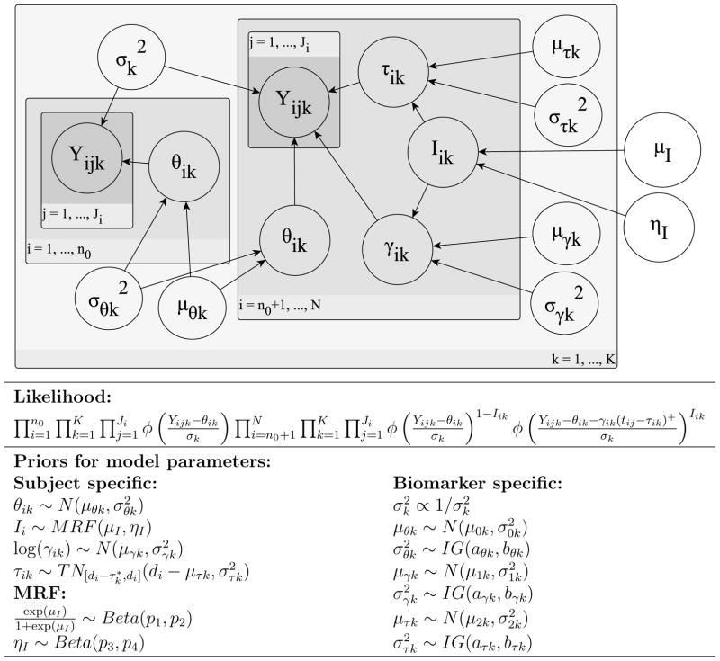
We complete the model assuming that the biomarker specific mean parameters (μ_θk, μ_γk and μ_τk) have normal priors and the variance parameters ( ${\sigma }_{\theta k}^2,{\sigma }_{\gamma k}^2$ and ${\sigma }_{\tau k}^2$) have inverse-gamma (IG) priors. In Figure 2, we provide a graphical representation of the assumed probabilistic model and a summary of the hierarchical structure.

Figure 2.

Graphical representation and hierarchical structure of probabilistic model.

3.3 Markov Chain Monte Carlo computational algorithm

The joint posterior distribution for all the parameters is not available in closed form hence we construct a Markov Chain Monte Carlo (MCMC) algorithm to sample from the posterior. We provide a brief outline of the MCMC procedure used here (see Web Appendix B.1 for full details). For most of the biomarker specific parameters ( ${\sigma }_k^2$, μ_θk, ${\sigma }_{\theta k}^2$, μ_γk, ${\sigma }_{\gamma k}^2$), the full conditional distributions are easily computed and we can employ a Gibbs sampler step. It is not straightforward to sample from the full conditional distributions of the biomarker specific parameters related to the change-point (μ_τk, ${\sigma }_{\tau k}^2$) or the MRF parameters (μ_I, η_I) thus we employ a Metropolis-Hastings step to obtain draws from the full conditional distribution.

For the subject-specific parameter θ_ik, we can use a Gibbs sampler since the full conditional distribution is easily computed. The posterior distributions for the subject-specific parameters I_ik, γ_ik and τ_ik are intrinsically connected and therefore we obtain draws from the full conditionals as detailed in the following strategy. If I_ik = 1, then we have three parameters θ_ik, γ_ik and τ_ik associated with the k^th biomarker of the i^th patient; but if I_ik = 0, then there is only one subject-specific parameter, θ_ik. Since the dimension of the parameter space depends on I_ik, a reversible-jump step (Green, 1995) is used to sample from the full conditional distribution of (I_ik, γ_ik, τ_ik).

3.4 Screening rule: Posterior risk calculation

The decision rule for a new (N + 1)^th patient at screening time t_ij is based on the posterior risk of disease, given the longitudinal history of each biomarker up to time t_ij, defined as

$$\frac{P(D_{N+1}=1\mid {\mathbf{Y}}_{N+1})}{P(D_{N+1}=0\mid {\mathbf{Y}}_{N+1})}=\frac{P({\mathbf{Y}}_{N+1}\mid D_{N+1}=1)}{P({\mathbf{Y}}_{N+1}\mid D_{N+1}=0)}\times \frac{P(D_{N+1}=1)}{1-P(D_{N+1}=1)},$$

where Y_N+1 = {Y_(N+1)j′k, j′ = 1, . . . , j and k = 1, . . . , K}.

The prior prevalence, P(D_N+1 = 1), could be estimated from training data or an external source when necessary. For example, we can more accurately estimate the prior prevalence from population registries when the surveillance program targets the general population. The components P(Y_N+1|D_N+1 = 1) and P(Y_N+1|D_N+1 = 0) are estimated via posterior predictive distributions for the (N + 1)^th patient’s marker levels given marker levels in the N training data patients. A Monte Carlo integration procedure is used to compute the probabilities. See Web Appendix B.2 for the full details.

If the posterior risk exceeds a pre-specified threshold then patient history indicates that the probability of being a case is sufficiently greater than the probability of being a control. The screening result is deemed positive and additional testing to detect the presence/absence of disease is recommended. In the case of HCC, a positive screen would result more sensitive imaging, such as CT or MRI. The appropriate threshold for the posterior risk depends on the disease context. If current practice results in all the patients undergoing additional testing, the screening goal is to “rule out” patients from additional testing and the threshold is chosen to maintain high sensitivity. In HCC screening, our goal is to “rule in” patients for additional testing and therefore the threshold is chosen to ensure a low false positive rate.

The standard measures to evaluate screening are based on a single test: sensitivity (proportion of cases with a positive test) and specificity (proportion of controls with a negative test). We extend these definitions to the longitudinal screening setting. Patient-level sensitivity is defined as the proportion of cases with at least one positive test during the screening period. Screening-level specificity is defined as the proportion of negative tests among all the screenings conducted in the control group. The specificity (1-false positive rate) is defined at the screening level because each false positive result leads to further testing that can be expensive and may lead to complications and anxiety.

4. Simulation Study

We compare our joint multivariate fully Bayesian screening algorithm (mFB-J) to existing univariate screening approaches: univariate fully Bayesian (uFB) screening (Skates et al., 2001), univariate parametric empirical Bayes (uEB) screening (McIntosh and Urban, 2003), and the standard threshold (ST) approach. The gains of jointly modeling are evaluated by including an independent multivariate fully Bayesian (mFB-I) screening algorithm that uses three biomarkers but assumes independent Bernoulli(π_k) priors for I_ik (k = 1, . . . , 3). See Web Appendix C for more details. The simulation study goal is to compare screening approaches, under a range of possible biomarker trajectories, and evaluate which has greater potential to increase early detection of HCC when used in clinical practice.

For each approach, we compare the full receiver operating characteristic (ROC) curve, ROC(0.1): patient-level sensitivity corresponding to 90% screening-level specificity (reported specificity for AFP in clinical practice (Marrero et al., 2009)) on the ROC curve, and the timing of the first positive screen. These measures quantify the potential of each screening algorithm to improve early detection of HCC from multiple perspectives.

We generate training data for model fitting (Section 3.3) and a validation dataset to implement screening (Section 3.4). The simulations were designed to mimic aspects of the HALT-C Trial data structure. Each dataset includes 400 patients (each a case with probability 50/400) followed longitudinally for up to 5 years. The screening visit time, t_ij, was every six months on average, with variability included to mimic patient behavior, and three biomarkers were measured at each visit. The length of follow-up was uniformly distributed between 0 to 5 years resulting in an unbalanced number of screening visits (J_i) for each patient.

The biomarker levels are simulated from the joint model (Section 3) for cases, with and without a changepoint, and controls. In scenario A (Table 1), we assume the first two markers have similar trajectories to AFP and DCP in the HALT-C study. The third biomarker had a slightly lower rate of increase after the change-point. In scenario B, we assume all three markers have lower rates of increase after their respective change-points. In scenario C, we assume that the first marker has the same trajectory used in scenario A while the other 2 markers have the flatter trajectory used in scenario B. These scenarios allow us to explore screening performance under a variety of trajectories for multiple markers. See Web Table 5 for parameter values for each scenario.

Table 1.

Summary of simulation results in 200 studies: empirical mean ROC(0.1) (empirical standard error of the mean). mFB-J: joint multivariate fully Bayesian, mFB-I: independent multivariate fully Bayesian, uFB: univariate fully Bayesian, uEB: parametric empirical Bayes and ST: single threshold. The mean biomarker trajectories assumed for each scenario are shown in column 1. Biomarker 1 (solid) and 2 (dashed) in scenario A were assumed to have trajectories similar to those observed for AFP and DCP respectively in the HALT-C study. Biomarker 3 (dotted) was assumed to lie between the two with a lower rate of increase after the changepoint. In scenario B and C, biomarkers 2 and 3 were assumed to have flatter slopes. Biomarker 1 was assumed to have a flatter slope in scenario B while in scenario C the assumed slope for biomarker 1 was the same as that used in scenario A.

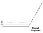
	Scenario A
	Biomarker	mFB-J	mFB-I	uFB	uEB	ST
	(1)			67.91 (0.49)	66.65 (0.49)	51.22 (0.56)
	(2)	81.58 (0.42)	81.44 (0.41)	63.78 (0.55)	62.70 (0.51)	55.23 (0.53)
	(3)			58.75 (0.51)	58.61 (0.48)	46.75 (0.50)
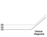
	Scenario B
	Biomarker	mFB-J	mFB-I	uFB	uEB	ST
	(1)			63.97 (0.48)	64.17 (0.46)	45.28 (0.51)
	(2)	72.12 (0.46)	71.83 (0.48)	54.34 (0.53)	54.18 (0.53)	44.87 (0.50)
	(3)			55.82 (0.57)	55.12 (0.50)	41.87 (0.54)
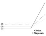
	Scenario C
	Biomarker	mFB-J	mFB-I	uFB	uEB	ST
	(1)			71.28 (0.45)	69.24 (0.47)	55.81 (0.50)
	(2)	77.68 (0.42)	77.45 (0.42)	54.63 (0.51)	54.79 (0.56)	45.23 (0.53)
	(3)			56.21 (0.53)	55.18 (0.45)	42.16 (0.49)

4.1 Results

In each of 200 simulation studies, the hyperparameters were kept consistent across each simulation scenario and are listed in Web Table 6. The draws from the posterior distributions were obtained from the MCMC algorithm applied in the training data. The parameters of the uEB screening algorithm were estimated from the training data (see Web Appendix C for more details). All screening algorithms were then implemented in the validation data.

The empirical mean ROC(0.1) and standard error of the mean are presented in Table 1. In all scenarios, we observe that the multivariate screening algorithms have significantly higher ROC(0.1) than the univariate approaches; the standard threshold performs worse than either uFB or uEB; and the uFB and uEB methods have comparable performance. Across scenarios we note (a) the performance of all methods decrease if the rate of increase after the changepoint is decreased (scenario A vs B); (b) increasing the slope of a single biomarker increases the performance of the corresponding univariate algorithms by a larger margin than the improvement in the multivariate algorithms (scenario B vs C) and; (c) introducing a 15% probability of a missed visit decreases the ROC(0.1) for all the methodologies (scenario A vs D in Web Table 7). If we fix the threshold in the training data, the conclusions remain the same (see Web Tables 8–9), which is expected since we are able to estimate the threshold for specificity with high precision with large numbers of controls.

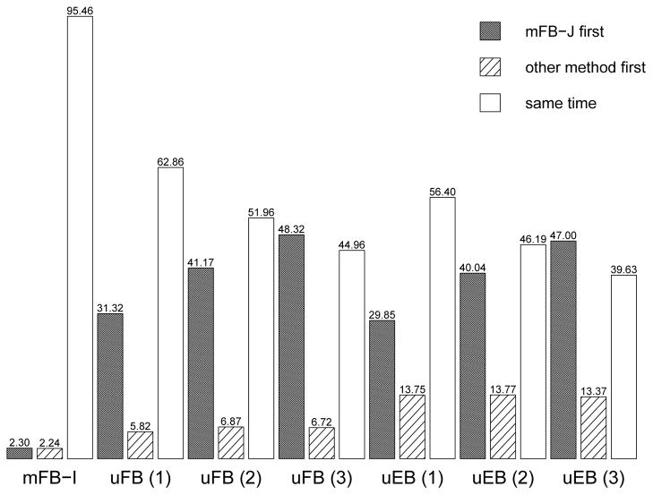
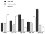
Next we compare which approach has a positive screen first to evaluate the likelihood of earlier detection in Scenario A. We define disease onset to be the earliest changepoint time and only consider patients whose disease is detectable using the biomarkers of interest, i.e at least one elevated marker measured after disease onset. A small subset of cases whose markers are not elevated are excluded. In Figure 3, we observe the mFB-J is more likely to have a positive screen first but there is little difference between the joint and independent approaches. In particular, the mFB-J approach has earlier positive screens (31.32% vs 5.82%) compared to uFB approach with marker (1), the “strongest” marker (highest sensitivity). When we compare the uEB and uFB approaches for marker (1), the uFB has a positive screen first 5.37% of the time while the uEB approach has a positive screen first 15.14% of the time (Web Table 10). Similar results were observed for markers (2) and (3).

Figure 3.

The bar height corresponds to the percentage of times: the proposed joint multivariate fully Bayesian (mFB-J) approach has a positive screen first, an alternative method has a positive screen first and the first positive screen for both methods is the same time after disease onset (Scenario A of the simulation study). mFB-I: independent multivariate fully Bayesian, uFB: univariate fully Bayesian and uEB: parametric empirical Bayes.

5. Results from the HALT-C Trial

The screening methods were evaluated in cirrhosis patients from the HALT-C Trial. Studies with serial AFP and DCP in cirrhosis patients are rare and we currently do not have an external validation dataset, hence 10-fold cross-validation is used to evaluate screening.

5.1 Joint model for log(AFP) and log(DCP+1)

The longitudinal trajectories of log(AFP) and log(DCP+1) are assumed to follow the joint model described in Section 3.1. The priors are outlined using general notation in Section 3.2. The hyperparameter values were chosen during exploratory analysis (Web Table 1).We chose relatively vague priors for parameters from the control model since there was substantial data on control patients. For parameters that were specific to the changepoint model for cases, we used more informative priors and examined the sensitivity of the results (Section 5.3).

We expect that AFP will increase after disease onset in about 50% of patients and similarly, DCP will increase after disease onset in about 50% of patients. Hence we specify the relatively informative prior exp(μ_I)/{1+exp(μ_I)} ~ Beta(30, 30). That is, the Beta prior of the logistic transformation of μ_I has mean 0.5 and standard deviation 0.064. The Beta prior of η_I had mean 0.1 and standard deviation 0.042 (η_I ~ Beta(5, 45)). The hyperparameters for both Beta priors are large enough to ensure stable MCMC chains but not too large given that the sum corresponds to the assumed sample size of prior information. When μ_I and η_I are set to their expected value, the prior probability that AFP has a changepoint is 0.65 if we observe a changepoint for DCP and 0.62 if we don’t observe a changepoint for DCP.

5.2 Model assessment

It is important to assess goodness of fit since the posterior distributions of the biomarker-specific parameters are needed for future posterior risk estimates. Each subject’s posterior predictive distribution was calculated by drawing from a Normal distribution with the mean functions described in Section 3.1 (using the subject-specific parameters θ_ik, I_ik, γ_ik and τ_ik) and variance ${\sigma }_k^2$. First we considered the model assumption that the trajectory of AFP and DCP in control patients is essentially flat (i.e slope is 0). In Web Figure 4, the first row displays the empirical distribution of the observed slopes for AFP and DCP that are tightly centered around 0 indicating a flat profile for AFP and DCP is appropriate. In the second row, we observe the average slope of AFP and DCP from the posterior predictive distributions are also tightly centered around 0 indicating the model slopes were also flat.

The mean profiles of the posterior predictive distribution and 95% intervals were used to examine model fit in HCC cases. The 95% intervals are calculated by computing the standard deviation (SD) of the posterior predictive draws at each time point and then adding and subtracting 1.96*SD from the mean profile. In Web Figure 12, we present the model fit for the HCC cases depicted in Figure 1 and note the model captures the changepoints.

A key model assumption is that the biomarker-specific variance ${\sigma }_k^2$ is constant. In Web Figure 13, we examine the residuals for the 48 cases (left column) and 361 controls (right column) in logarithmic scale. For both AFP and DCP, there is no evidence of trends over time and we conclude that the assumption of constant biomarker-specific variance is justified.

5.3 Prior sensitivity

The sensitivity to the prior distributions was assessed by evaluating how the posterior probability of an AFP and DCP changepoint varied in the 48 HCC cases under three different priors for η_I, μ_I, μ_γ and μ_τ (Web Figures 6–9). The posterior probability of a changepoint is an important component of the model fit that affects the performance of the screening.

As we increase the η_I prior’s mean (Web Figure 6), we increase the connection between the markers. For those with a high posterior probability of a changepoint for one marker, increasing η_I increases the posterior probability of a changepoint for the other marker. For borderline values (between 0.5–0.7), a higher prior mean pulls both posterior probabilities of changepoints upwards. In μ_I (Web Figure 7), we observe more sensitivity in the posterior probability of changepoints to changes in the prior’s mean but the rankings of patients are mostly preserved. Spearman’s rank correlation was ~ 0.99 and ~ 0.96 for AFP and DCP respectively, indicating the posterior inference is robust to moderate changes.

The posterior probability of changepoints are sensitive to the μ_γ prior (Web Figure 8). We observe an inverse relationship between μ_γ prior’s mean and the posterior probability of changepoints for AFP and DCP. The rankings of the posterior probabilities of a changepoint are preserved for AFP (Spearman’s rank correlation: > 0.99) but not always for DCP (Spearman’s rank correlation: 0.62–0.85). Since we have reduced follow-up for DCP, we expect the prior selection is crucial. For μ_τ (Web Figure 9), we observed minimal sensitivity of the posterior probabilities of changepoints to changes in the mean of the prior.

5.4 Cross-validated analysis

The proposed screening methodology performance was evaluated in the HALT-C Trial via 10-fold cross-validation. 361 control patients were randomly divided into nine subsets of 36 patients and one subset of 37 patients. 48 HCC cases were randomly divided into eight subsets of 5 patients and two subsets of 4 patients. At each iteration of the cross-validation, the validation data consists of one subset of HCC cases and one subset of controls. The remaining nine subsets of cases and controls form the training data. The MCMC procedure (Section 3.3) was applied to the training data to estimate the posterior distributions of parameters in a joint model of log(AFP) and log(DCP + 1). The MCMC algorithm was run for 50,000 updates after a burn-in period of 2000 iterations. For each analysis, we ran two separate chains. To reduce autocorrelation, each chain was thinned and only every 10 updates were retained. Convergence of the MCMC chains was assessed via traceplots (Web Figure 9–10) and Gelman-Rubin statistics. Posterior inference for screening (Section 3.4) was then applied in the validation data.

For the ST approach, we identify AFP and DCP thresholds corresponding to 90% screening-level specificity in the training subset, calculate the patient-level sensitivity and screening-level specificity in the validation subset and average the results across each iteration. We estimate the ST approach has patient-level sensitivity and screening-level specificity of 59% and 89.17% respectively for AFP and 54.66% and 89.06% respectively for DCP.

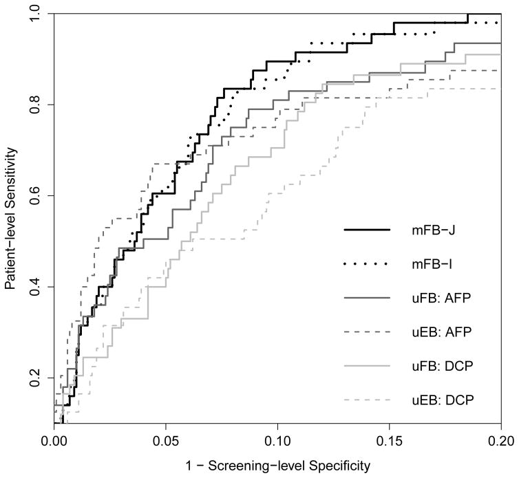
In Figure 4 we present the cross-validated ROC curves, calculated by averaging the patient-level sensitivity across each iteration at a fixed screening-level specificity based on the entire screening period. The ROC curves for the joint screening approaches lie above those for the univariate approaches within the range of potential targets for screening-level specificities (80–90%) used in HCC screening among high-risk cirrhosis patients.

Figure 4.

Cross-valiated ROC curve for mFB-J: joint multivariate fully Bayesian, mFB-I: independent multivariate fully Bayesian, uFB: univariate fully Bayesian and uEB: parametric empirical Bayes. The ROC curve for screening-level specificity between 0.8 and 1 is shown (See Web Figure 10 for full ROC curve).

We also consider the performance of the screening approaches within 1 or 2 years prior to clinical diagnosis. These are the periods during which a positive screen is more likely to lead to confirmation of HCC diagnosis using more sensitive imaging (CT or MRI). In Table 2 we highlight the patient-level sensitivity corresponding to 90% screening-level specificity for each longitudinal screening method during the three different time periods.

Table 2.

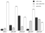
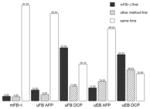
Cross-valiated ROC(0.1) for mFB-J: joint multivariate fully Bayesian, mFB-I: independent multivariate fully Bayesian, uFB: univariate fully Bayesian and uEB: parametric empirical Bayes in the three time periods. In each figure, the bar height corresponds to the percentage of times: the mFB-J approach has a positive screen first, an alternative method has a positive screen first and the first positive screen for both methods is the same time in the three time periods.

Time Period	Biomarker	mFB-J	mFB-I	uFB	uEB
Entire screening period	log(AFP) log(DCP+1)	89.50%	85.50%	81.00% 70.50%	7.00% 60.50%
2-year prior to clinical diagnosis	log(AFP) log(DCP+1)	60.50%	62.50%	56.00% 43.52%	60.00% 58.33%
1-year prior to clinical diagnosis	log(AFP) log(DCP+1)	59.50%	59.50%	53.00% 43.52%	57.00% 56.48%

At 90% screening-level specificity, we observe that the longitudinal screening approaches with AFP have higher sensitivity than DCP, but this is not a fair comparison. As described in Section 2, DCP was measured in an ancillary study to the HALT-C Trial and is only available up to 42 months post-randomization. For all those HCC cases diagnosed in the extended follow-up period of the study, we do not have DCP at screening times leading up to clinical diagnosis. While it is an advantage of our approach that we can still implement the joint screening algorithm, this study design reduces the chance of DCP “detecting” HCC.

We compare the first positive screen time across the different approaches. In Table 2, we observe that while the mFB are more likely to have a positive screen first compared to the uFB approaches in all three time periods, the uEB approach with AFP is more likely to have a positive screen first within one and two years of clinical diagnosis. In addition, the uEB approach with AFP has comparable patient-level sensitivity to the joint screening approaches in these time periods. This result indicates that the mFB-J method is potentially more useful for determining longer term risk of HCC, while the uEB with AFP is potentially more useful for shorter term risk prediction, although it is unknown how the two approaches will compare if DCP has the same extent of serial measurement and if elevated AFP was not used for triggering work-ups to diagnose HCC (see Web Tables 2–4 for all possible comparisons).

6. Discussion

A critical component towards reducing mortality associated with HCC is detecting the disease at an early stage when there are more treatment options available. Detecting HCC prior to any clinical symptoms requires surveillance programs in high-risk cirrhosis patients. Currently, all cirrhosis patients are recommended to undergo ultrasonography (that is operator dependent and therefore not reliable in detecting early lesions in practice) with or without measurement of AFP (that has limited sensitivity) every six months. Surveillance adherence is reported to be around one-third (Singal et al., 2011), which contributes to the high mortality associated with HCC. In addition to improving the performance of the surveillance tests, patient outcomes could also be improved by better identifying cirrhosis patients at higher risk of HCC and ensuring compliance among these patients.

The proposed fully Bayesian screening approach with longitudinal AFP and DCP had the highest detection rate with at-least one positive screen in 89.5% of the HCC cases, while maintaining a 10% false positive rate in all the screenings conducted in the control patients in the HALT-C Trial. The proposed method was also more likely to have a positive screen first during the entire screening period. In the 1–2 year prior to clinical diagnosis, we observed that the parametric empirical Bayes method with AFP had comparable levels of sensitivity to the proposed approach and was more likely to have a positive screen first. We conclude the two approaches could each have better performance in different but complementary areas: long term and short term risk identification, but with two caveats. First, evaluating the added value of DCP is limited due to the shorter serial follow-up; and second, elevated AFP triggered some of the work-ups to diagnose HCC which may put the the approach using both AFP and DCP at a disadvantage. Further studies in cohorts with blood collection to allow retrospective measurement of AFP and other biomarkers, where AFP is not used for surveillance, are needed to clarify this observation.

The methodology we have developed will be applied to data from multiple ongoing longitudinal studies of HCC screening in cirrhosis patients. In particular, The Texas Hepatocellular Carcinoma Consortium (THCCC) will assemble the largest prospective cohort study of cirrhosis patients to study early detection of HCC in the United States. They will be collecting longitudinal AFP, DCP and other novel biomarkers for HCC. The EDRN HEDS cohort has already recruited more than 1,400 cirrhosis patients and will include five-year follow-up during which AFP, DCP and other emerging biomarkers will be measured longitudinally. These two cohorts will provide a rich resource to further study HCC screening with multiple longitudinal biomarkers and have the potential to advocate for changes to the current HCC screening practice guidelines.

There are methodological challenges to jointly modeling the trajectories of multiple biomarkers. We have chosen to connect the biomarkers by jointly modeling the unobserved changepoint indicator (I_ik). In sensitivity analysis, we found that the posterior inference was robust to moderate changes in the hyperparameters of the MRF prior. This is a very desirable property of our approach because it implies that the performance of the screening will also be robust to the prior assumptions. In future work, we could develop models that also consider jointly modeling the rate of increase after the changepoint (γ_ik) or the changepoint time (τ_ik) that may be useful in other settings. In our current study we have not chosen to take this approach for two reasons: (1) we are limited by the data (48 HCC cases) and (2) we currently do not have any scientific reason to jointly model these parameters.

Additional future work will explore multiple extensions to our model. We will modify our model to incorporate covariates that can potentially affect biomarker levels, such as age, gender, race, and other liver function markers. In the more general populations of the THCCC and EDRN HEDS cohorts, where larger numbers of HCC cases are expected, the etiology of cirrhosis could be an important covariate to include in the biomarker models. We will also consider relaxing some of our model assumptions, such as constant biomarker-specific variance (σ_k) on logarithmic scale. In the HALT-C Trial, this assumption appears reasonable but we may need to consider time-varying variance or covariates that affect biomarker variability in future studies. A simulation study was conducted (Web Table 11) and we found that our proposed fully Bayesian screening methodology was robust to linear increases in biomarker variability after the changepoint. Future work will further examine the robustness of our proposed methodology when there are covariates that affect the biomarker-specific variance. We will also explore extending our methodology to accommodate more general trajectories, such as the approach taken by Chib (1998). This may be important area of future research when we want to include novel HCC markers whose trajectories during the pre-clinical phase are not well studied and likely to be unclear.

While it is methodologically challenging to develop screening methods for multiple longitudinal biomarkers, this is an important area of research that has practical implications for clinical practice in HCC. We have added to the field by proposing an approach that begins to tackle this problem. We have also provided R-code for the univariate fully Bayesian method (Skates et al., 2001), the parametric empirical Bayes method (McIntosh and Urban, 2003) and our proposed multiple biomarker method in order to promote the more widespread usage of these screening algorithms.

References

- Bruix J, Sherman M. Management of hepatocellular carcinoma. Hepatology. 2005;42:1208–1236. doi: 10.1002/hep.20933. [DOI] [PubMed] [Google Scholar]
- Bruix J, Sherman M. Management of hepatocellular carcinoma: An update. Hepatology. 2011;53:1020–1022. doi: 10.1002/hep.24199. [DOI] [PMC free article] [PubMed] [Google Scholar]
- Chib S. Estimation and comparison of multiple change-point models. Journal of Econometrics. 1998;86:221–241. [Google Scholar]
- Drescher CW, Shah C, Thorpe J, O’Briant K, Anderson GL, Berg CD, Urban N, McIntosh MW. Longitudinal screening algorithm that incorporates change over time in ca125 levels identifies ovarian cancer earlier than a single-threshold rule. J Clin Oncol. 2013;31:387–392. doi: 10.1200/JCO.2012.43.6691. [DOI] [PMC free article] [PubMed] [Google Scholar]
- El-Serag HB. Hepatocellular carcinoma. N Engl J Med. 2011;365:1118–1127. doi: 10.1056/NEJMra1001683. [DOI] [PubMed] [Google Scholar]
- Gebo KA, Chander G, Jenckes MW, Ghanem KG, Herlong HF, Torbenson MS, El-Kamary SS, Bass EB. Screening tests for hepatocellular carcinoma in patients with chronic hepatitis c: A systematic review. Hepatology. 2002;36:s84–s92. doi: 10.1053/jhep.2002.36817. [DOI] [PubMed] [Google Scholar]
- Green PJ. Reversible jump markov chain monte carlo computation and bayesian model determination. Biometrika. 1995;82:711–732. [Google Scholar]
- Lee E, Edward S, Singal AG, Lavieri MS, Volk M. Improving screening for hepatocellular carcinoma by incorporating data on levels of α-fetoprotein, over time. Clin Gastroenterol Hepatol. 2013;11:437–440. doi: 10.1016/j.cgh.2012.11.029. [DOI] [PubMed] [Google Scholar]
- Lok AS, Everhart JE, Wright EC, Di Bisceglie AM, Kim HY, Sterling RK, Everson GT, Lindsay KL, Lee WM, Bonkovsky HL, Dienstag JL, Ghany MG, Morishima C, Morgan TR. Maintenance peginterferon therapy and other factors associated with hepatocellular carcinoma in patients with advanced hepatitis C. Gastroenterology. 2011;140:840–849. doi: 10.1053/j.gastro.2010.11.050. [DOI] [PMC free article] [PubMed] [Google Scholar]
- Lok AS, Sterling RK, Everhart JE, Wright EC, Hoefs JC, Di Bisceglie AM, Morgan TR, Kim HY, Lee WM, Bonkovsky HL, Dienstag JL. Des-gamma-carboxy prothrombin and alpha-fetoprotein as biomarkers for the early detection of hepatocellular carcinoma. Gastroenterology. 2010;138:493–502. doi: 10.1053/j.gastro.2009.10.031. [DOI] [PMC free article] [PubMed] [Google Scholar]
- Marrero JA, Feng Z, Wang Y, Nguyen MH, Befeler AS, Roberts LR, Reddy KR, Harnois D, Llovet JM, Normolle D, Dalhgren J, Chia D, Lok AS, Wagner PD, Srivastava S, Schwartz M. α-fetoprotein, des-γ carboxyprothrombin, and lectin-bound α-fetoprotein in early hepatocellular carcinoma. Gastroenterology. 2009;137:110–118. doi: 10.1053/j.gastro.2009.04.005. [DOI] [PMC free article] [PubMed] [Google Scholar]
- McIntosh MW, Urban N. A parametric empirical bayes method for cancer screening using longitudinal observations of a biomarker. Biostatistics. 2003;4:27–40. doi: 10.1093/biostatistics/4.1.27. [DOI] [PubMed] [Google Scholar]
- Norris M, Johnson WO, Gardner IA. Modeling bivariate longitudinal diagnostic outcome data in the absence of a gold standard. Statistics and its Interface. 2009;2:171–185. [Google Scholar]
- Singal AG, Volk ML, Rakoski MO, Fu S, Su GL, McCurdy H, Marrero JA. Patient involvement in healthcare is associated with higher rates of surveillance for hepatocellular carcinoma. Journal of clinical gastroenterology. 2011;45:727–732. doi: 10.1097/MCG.0b013e31820989d3. [DOI] [PubMed] [Google Scholar]
- Skates SJ, Pauler DK, Jacobs IJ. Screening based on the risk of cancer calculation from bayesian hierarchical changepoint and mixture models of longitudinal markers. JASA. 2001;96:429–439. [Google Scholar]
- Sterling RK, Wright EC, Morgan TR, Seeff LB, Hoefs JC, Di Bisceglie AM, Dienstag JL, Lok AS. Frequency of elevated hepatocellular carcinoma (HCC) biomarkers in patients with advanced hepatitis C. Am J Gastroenterol. 2012;107:64–74. doi: 10.1038/ajg.2011.312. [DOI] [PMC free article] [PubMed] [Google Scholar]
- Tayob N, Lok AS, Do KA, Feng Z. Improved detection of hepatocellular carcinoma by using a longitudinal alpha-fetoprotein screening algorithm. Clinical Gastroenterology and Hepatology. 2016;14:469–475. doi: 10.1016/j.cgh.2015.07.049. [DOI] [PMC free article] [PubMed] [Google Scholar]
Associated Data
This section collects any data citations, data availability statements, or supplementary materials included in this article.