Abstract
Haptic feedback is a critical but a clinically missing component in robotic Minimally Invasive Surgeries. This paper proposes a Gaussian Process Regression(GPR) based scheme to address the gripping force estimation problem for clinically commonly used elongated cable-driven surgical instruments. Based on the cable-driven mechanism property studies and surgical robotic system properties, four different Gaussian Process Regression filters were designed and analyzed, including: one GPR filter with 2-dimensional inputs, one GPR filter with 3-dimensional inputs, one GPR Unscented Kalman Filter (UKF) with 2-dimensional inputs, and one GPR UKF with 3-dimensional inputs. The four proposed methods were compared with the dynamic model based UKF filter on a 10mm gripper on the Raven-II surgical robot platform. The experimental results demonstrated that the four proposed methods outperformed the dynamic model based method on precision and reliability without parameter tuning. And surprisingly, among the four methods, the simplest GPR Filter with 2-dimensional inputs has the best performance.
Index Terms: Sensorless Grip Force Estimation, Elongated Cable Driven Instrument, Gaussian Process Regression, Surgical Robot, Minimally Invasive Surgery
I. INTRODUCTION
SURGICAL robots extended applications of minimally invasive surgery(MIS) by providing surgeons with improved freedom of movement, decreased hand tremor, increased accessibility and advanced 3-dimensional imaging[1], [2]. Haptic perception is still a missing component clinically[3] in robotic MISs, because of the challenge of the problem. However, haptic perception is highly desirable, because surgeons rely on it to diagnose and to adapt their motion to prevent unintended tissue damage or task failure.
The most straightforward way to perceive haptic force is to use sensors to directly measure the force on instrument tips. For minimally invasive surgery instruments, the stringent size, cost, and environmental requirements prevented the application of these techniques. Although various sensors broke the size limitation [4], [5], [6], they are still not widely available due to the cost, sterilization requirements and other factors. It is also possible to “indirectly” measure tip force through novel mechanical designs. For example, Tholey et al. designed a novel laparoscopic tool with tri-directional force measurement capability at the grasping jaws[7], and the disturbance observer was applied to estimate the force [8]. Zhao et al. proposed and developed a novel 3-DoFs robotic surgical tool to estimate tool-tissue forces through force-sensitive resistors[9]. These new designs are very useful, but they also increased the complexity and the cost, and haven’t been widely adopted clinically. An in-depth discussion on the advantages and disadvantages of solutions to the force perception problem can be found in[3].
It is possible to achieve the active gripping force of a surgical instrument without adding sensors, since active gripping forces originate from motor output torques. For some deformable instruments, the interaction force can be estimated through measuring the instrument deformation. For example, Khoshnam et al. used the shape changes of the Steerable Ablation Catheters to estimate the contact forces between the catheter tip and cardiac tissue[10]. For rigid instruments, such as elongated grippers, motors drive cables and the output energy of motors is partially consumed by friction, converts to kinetic energy and forms the gripping force. Although it is clear that dynamic model describes the process of energy exchange and conversion, it is not trivial to apply this idea to the force estimation problem, as some of the factors mentioned above, such as friction and cable properties, are difficult to model. Friction is a phenomenon arising at the contact of surfaces, and experiments indicate a functional dependence upon a large variety of parameters, for example: sliding speed, acceleration, critical sliding distance, temperature, normal load, humidity, surface preparation, and material combination [11]. Anooshahpour et al. proposed a smart way to minimize the impact from the friction and from the movement by constructing the dynamic model of the da Vinci instrument under the quasi-static condition[12]. Research demonstrated that cable stretch and friction depend on cable properties[13], [14], [15]. Based on these studies, Li et al. applied the square root Unscented Kalman Filter to estimate the gripping force through incorporating cable properties, cable friction and cable-pulley friction into the dynamic model[16]. However, it has been found that as friction and cable properties have big weights in the model, the method is sensitive to the model parameters[16], which depend on both system configuration and environment. For example, model parameters change dramatically with instrument type and lubrication condition. Manually tuning these parameters for each instrument under various environmental conditions is very tedious and undesirable. Moreover, the effort[16] on on-line parameter estimation was not successful due to the fact that there are dozens of parameters and dozens of state variables and only 8 observations are generally available (4 motor torque outputs and 4 motor encoder readings for a wristed gripper).
In order to extend the application of the sensorless gripping force estimation to elongated cable driven surgical instrument, in this paper, we propose to simplify the estimation algorithm and to further improve estimation precision by learning the model from training data. Gaussian Process Regression was adopted in the paper because of its ability to deal with uncertainties and nonlinearity[17]. Four different designs of Gaussian Process Regression filters are proposed, and estimation precision will be compared on real surgical instruments and surgical robots. To sum up, the core contributions of the paper are:
We propose four Gaussian Process Regression filters, (which have no free parameters), for sensorless gripping force estimation, based on characteristics of elongated cable driven surgical instruments.
We implemented the proposed filters and applied them on a 10mm gripper with the Raven-II robot;
We compared the four proposed methods with the dynamic model based UKF estimator on dry lab experiments with the real robot, validated the precision and reliability of the proposed methods, and identified the method of the best performance.
The paper is organized as follows: Section II presents preliminaries for the proposed methods; Section III explains the methods used for sensor-less force estimation in detail; Section IV presents and discussed the experiment setup and the experimental results. Conclusions are summarized in Section V.
II. Preliminaries
A. Elongated Cable Driven Surgical Instruments
Before presenting the proposed algorithms, we briefly introduce elongated cable-driven surgical instruments, discuss their properties, and show the reasons that data driven learning algorithms were adopted in the paper.
Motorized surgical instruments adopted the cable driven mechanism because of the advantages of easy sterilization, small size and narrow aspect ratio[18]. An example 10mm diameter gripper can be seen in reference [16] Fig. 3. These cable-driven surgical instruments can be modeled as shown in Fig. 1.
Fig. 3.
Gaussian Process Regression for Elongated Cable-driven Surgical Instrument Sensorless Grip Force Estimation.
Fig. 1.
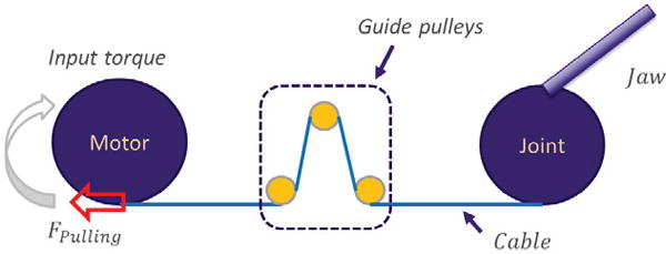
Elongated Cable Driven Surgical Instrument Model.
The dynamic model describes how a instrument exerts force on an object and exchanges energy. The dynamic model can be mathematically expressed as:
| (1) |
Where: A is the Inertia matrix of the manipulator; J is the Jacobian projecting external force into the reference coordinates; C(·) denotes the vector of Coriolis and centrifugal torques; G is the vector of gravitational force; q, , are the manipulator position, velocity and acceleration, respectively; Fv,Fc are viscous friction and coulomb friction parameters, respectively; and Γ,Fex are joint input torque and external torque (gripping force in our application) respectively.
Because of the cable driven mechanism, the relationship between the motor and the joint can be described as:
| (2) |
Where: qm, , : denote motor position, velocity and acceleration, respectively; ql, : denote link position and velocity; Am: denote the diagonal motor inertia matrix; Cm(·) denotes the vector of Coriolis and centrifugal torques in motor·coordinates; Fvm,Fcm are viscous friction and coulomb friction parameters, respectively; rm,rl: are capstan radius of motor and link, respectively; γ: is the cable tension. And fcs(·) and fcd(·) are the functions that describe the spring and damping effect, respectively. The explicit form of these two functions depend on cable properties[16], [14].
From Eqn. 1 and 2 we can easily see that the total number of parameters (6 friction related parameters plus 3 cable properties related parameters for each link) is bigger than the total number of state variables (6 state space variables for each link). And both of them are much bigger than the total number of available observations (2 observations for each link). Given the complexity of the dynamic model, it was not trivial to tune these parameters without extra sensors. More importantly, our previous research shown that the parameters depend on the system configuration and environmental conditions[16]. Therefore, this work was inspired by these difficulties and aimed to increase the adoption rate by simplifying the technique.
B. Gaussian Process Regression
Gaussian Process Regression(GPR) is a form of supervised learning[17]. GPR is similar to Bayesian Linear Regression(BLR) (see chapter 3.3 in [19]) in the sense that both of them aim at probabilistically estimating the expected output Y∗ given input X∗ with respect to the training set (X,Y) under the Bayesian framework as: p(Y∗|X*,X,Y) where we denote the relationship between the input X and output Y as . According to the Bayesian framework, we have p(Y∗|X∗,X,Y) = ∫p(Y∗|X∗, f)p(f|X,Y)df. If we assume the prior of the model was p(f), then the posterior of f given training data was , and the likelihood p(Y|X f) can be inferred from the training data. For example, in the Bayesian Linear Regression case, since the state space function f (X) was linear as f (X) = XT w, we have , where I was an identity matrix, X is a n × k design matrix and w is a k × 1 weight vector[19].
In contrast to BLR, Gaussian Process Regression uses kernels to represent the model, instead of explicitly adapting specific linear models. This kernel based scheme allows the data “speak” for themselves, which leads to the biggest difference between GPR and BLR. The power of GPR originates from the concept of Gaussian process and the kernel based learning scheme. A Gaussian process is a collection of random variables, any finite number of which follows a joint Gaussian distribution. A Gaussian process is completely specified by its mean function, m(X), and covariance function K, as f (X) ~ GP(m(X),K). Because of the definition of Gaussian Process, we have
. Therefore, the prediction Y∗ given the known data Y is , where
K∗ = (k(X∗,X1) ⋯k(X∗,Xn)), and K∗∗ = k(X∗,X∗) are all calculated according to the selected Gaussian Kernel. Kernel selection for the GPR will be discussed below. The kernel based learning scheme is another important reason that GPR suits nonlinear applications. In order to easily understand this difference, we can safely conclude that the advantage of GPR over BLR is similar to the advantage of Kernel based methods over the corresponding linear methods. However, this kernel based learning scheme limited the ability to “predict” if the prediction happens far away from seen data. Consequently, in GPR, it will produce high uncertainties with these predictions. In out applications, this can be seen as an advantage, because it is easy to achieve training data that covers the entire workspace, and if the prediction happens out of the range, it is better to let users know the prediction is not confident rather than being overconfident.
C. Unscented Kalman Filter
Unscented Kalman Filter addressed the linearization approximation problem of the Kalman Filter with the unscented transformation[20]. For the nonlinear state space function Y = f (X), assume X is L dimensional and had mean E(X) and covariance P, a L × (2L + 1)matrix composed of 2L + 1 sigma vectors χi formed with corresponding weights Wi:
| (3) |
| (4) |
, and λ = α2(L + κ) − L is a scaling parameter controlled by empirically determined parameter α and κ. The sigma points then are propagated through the nonlinear state space function to calculate the corresponding outputs γi = f (χi),i = 0, ⋯,2L, which are used to recover the posterior estimation.
The Gaussian Process Regression and the Unscented Kalman Filter were adopted in the paper because:
It is easy to get the training data for our application.
Gaussian Process Regression has outstanding ability to learn models for strongly nonlinear applications.
Gaussian Process Regression naturally estimates uncertainties, which is very important to increase the system ability of the teleoperation haptic feedback system.
It is not necessary to manually tune parameters of Gaussian Process Regression in our application.
Unscented Kalman Filter has outstanding ability to handle nonlinearity problem.
Unscented Kalman Filter does not require the derivatives of the model, only propagating sigma point is needed, therefore, it can be easily combined with GPR.
III. Gaussian Process Regression for Sensorless Grip Force Estimation
A. Gaussian Process Regression Force Estimation
Designing Gaussian Process Regression filters depends on the selection of the feature space. For motorized surgical instruments, motor encoder readings and motor output torques approximated by current sensing are always available. Therefore, naturally, encoder readings and output torque could be the inputs to the Gaussian Process Regression filter, and the gripping force should be the output. Mathematically, by following the denotations in Section II-B, we have X = {qm,Γ} as the training input data and Y = {Fex} as the output data. qm, Γ and Fex are explained in Eqn. 1 and 2. D = {X,Y} then is the training data.
The dynamic model of the elongated surgical instrument, which was mathematically explained in Eqn. 1 and 2, suggests that the gripping force not only depends on motor position and motor output torque, but also depends on motor velocity , joint position ql, and joint velocity . Therefore, the feature space formed by these variables should be better than the space formed only by qm and Γ. Consequently, the estimation precision should be improved[17], [21]. However, the joint position and velocity are not observed in the process due to the lack of external sensors, and their estimation depend on cable properties[14], [22]. As one of the goals of this work is to explore the possibility of avoiding manually tuning cable parameters, we consider ql and as unavailable. On the other hand, the motor velocity could be considered as available, because the motor encoders of our surgical robot produce high precision output, and with a simple filter, such as a Kalman Filter, the velocity can be easily estimated, as shown in Fig. 2. From the figure we can see that the raw observation and the integration of estimated velocity are almost identical (approximately delayed for one sampling period), which suggests we achieved desirable estimation precision. However, we know the velocity estimation directly depends on the position observations. Therefore, theoretically, the position observations have been used twice and may cause the overconfidence problem.
Fig. 2.
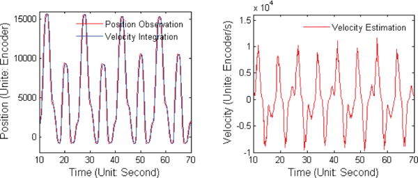
Motor Velocity Estimated with Kalman Filter based on Position Observation.
The next step of the proposed methods was to select the proper kernel function and the corresponding parameters. In the proposed methods, the popular widely used squared exponential kernel was adopted, because clear physical meanings for each parameter can be found in our application. The kernel is defined as: , where δ(X,X′) is the Dirac delta function defined as: . And M = l−2I, where l is a vector of positive values. In the model, l is the characteristic length-scale. In the proposed methods, l is small (l = 1.2 in the experiments) because it is easy to get training data and we have high resolution in the range of workspace. And σf and σn correspond to the process noise and the observation noise, respectively. In the proposed methods, σf and σn are selected bigger than the real dynamic model noises, (σf = 0.3, σn = 0.6 in the experiments) in order to safely “learn” from the training data. The process noise model depends on the system properties. For the gripper controlled by Raven II robot, from reference [14] we know 0.3×3 radian is far bigger than the true process noise. The observation noise model depends on the measurement sensor property, and the measurement noise of the sensor we adopted can be found in reference [16] Fig. 11. Please notice GPR does require normalizing features into similar ranges, just like other learning algorithms do, therefore, if the range of features change dramatically, these values should be changed accordingly. The experiments shown both the adopted kernel and the initial parameters worked well, mainly due to the good continuity.
Fig. 11.
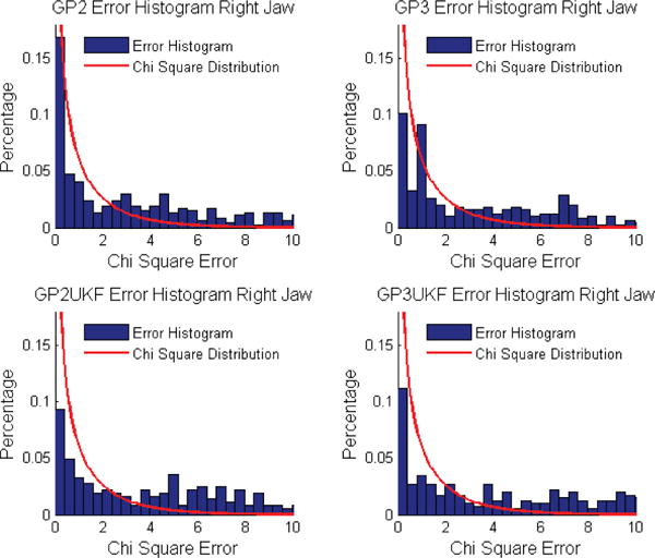
χ2 Error and Distribution Comparison for Right Jaw Force Estimation.
B. UKF and Gaussian Process Regression Force Estimation
In Section II-C we mentioned that UKF avoids explicitly linearizing the state space function through the introduction of the concept of sigma points. This new feature increases its robustness against strong nonlinearity and the poor priors. It has been reported that UKF can be combined with GPR, and the results outperformed the classical dynamic model based UKF in blimp tracking[23]. It was interesting to test if the combination of UKF and GPR can outperform GPR on precision for the gripping force estimation problem.
Applying GPR to UKF was simple. In the training phase, there is no difference between the GPR and the GPR based UKF, they share the same GPR and use the exactly same learning scheme. In the estimation phase, the GPR based UKF produce 2L+1 sigma points according to Eqn. 4. And 2L+1 estimations, denoted as γi, are generated through passing the sigma points through the trained GPR. The posterior of estimation can be recovered from γi as:
, where the weights Wm and Wc are calculated according to Eqn. 4, and the covariance P is calculated for generating sigma points at the next time point. The pseudocode of the GPR based UKF was listed in Algorithm.1.
Algorithm 1.
UKF&GPR for Grip Force Estimation
| Train GPR with training data (X,Y) | |
| Calculate sigma points χt−1 = {χt−1,i},i = 0, ⋯, 2L of X* according to Eqn. 4 | |
| Pt|t−1 = Pt−1 + Qt | |
| for i = 0, ⋯,2L do | |
| Calculate γt−1,i = GP(χt−1,i) | |
| end for | |
|
| |
|
|
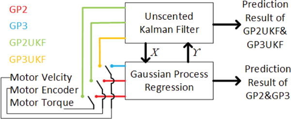
Through the discussion we know that because of the selection of different learning scheme and feature spaces, we have four GPR based filters for the sensorless gripping force estimation problem. Firstly, we can use two types of inputs. One is two dimensional and is composed of motor torque and motor encoder, and the other one is 3-dimensional and is composed of motor torque, motor encoder and motor velocity. Secondly, we have two types of estimator architectures. One is the classical GPR and the other one is the GPR based UKF. The difference between the two is the GPR based UKF uses GPR as the dynamic model. The combination of two input types and two architectures leads us to four estimators. For simplicity, we refer to the GPR with two dimensional inputs as GP2, the GPR with three dimensional inputs as GP3, and the GPR based UKF with two dimensional inputs as GP2UKF, the GPR based UKF with the three dimensional inputs as GP3UKF. For clarity, the differences among the four types of estimators are also visualized in Fig. 3.
IV. Experimental Result and Discussion
The four proposed methods were implemented and compared with the dynamic model based estimator on a 10mm diameter, cable-driven surgical gripper (can be seen in reference [16] Fig. 3) on the Raven-II surgical robot. The Raven-II robot was also fully driven by cables. This paper focused on the instrument gripping force estimation. Therefore, in the experiments reported here, the Raven manipulator held still and only the instrument moved. The experimental platform can be seen in Fig. 4
Fig. 4.
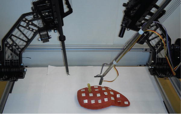
Sensorless Force Estimation Experiment Setup. A 10mm diameter, cable-driven surgical gripper was equipped with two force sensors (FSS015WNSB, Honeywell) on each of the two jaws. The gripper was driven by Raven II surgical robot and moved repeatedly and grasped a flexible latex rubber tube, which simulates blood vessel.
Two force sensors (FSS015WNSB, Honeywell) were mounted on the tip of the gripper to directly measure forces, as shown in reference [16] Fig. 3. Two aprons that rotated with respect to the jaw joint were added to the gripper in order to eliminate uncertainties from movable contact position. The gripper was statically calibrated with weights that range from 0N to 2N, and linear fit results were:
| (5) |
Detailed calibration information and usage can be found in [24], [16]. The gripping force was defined as the contact force between the object and the gripper jaw, which matches the sensor measurements. Given the definition, we know that the two forces on the left jaw and the right jaw are not equal, because of gravity, unsymmetrical contacting position and other factors.
A. Zero Grip Force Estimation Study
The proposed method was first verified with zero gripping force: the jaws repeatedly opened and closed, without touching each other or any other objects. Sensor measurements were compared with estimation results, while we know the true ground truth was nearly zero everywhere. The results are visualized in Fig. 5. The statistical results are compared in Table I. The results clearly show that estimations from both the four proposed methods and the dynamic model based method were smoother than sensor measurements, and the mean, the standard deviation, the threshold of 99% of data and the maximum error of the four proposed methods were very close to each other and outperformed the dynamic model based method. The results also shown the sensor measurements were noisy. A commercial force sensing unit, such as ATI Nano, are less noisy, but as we need to verify the proposed method in real movements, the instrument tips can be be fixed to a sensing unit. An alternative way is to estimate contacting position on-line, and convert torque to contact force. The current setup is chosen because: 1, the precision of estimating contacting point; 2, gripping a non-rigid object (rubber tube in our experiments) is preferable, as it better simulates real surgeries; 3, measurement error is high spikes and can be easily filtered out. An uncertainty based smoothing method was adopted to remove error spikes[25].
Fig. 5.
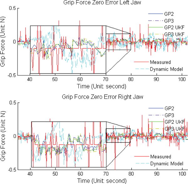
Non-gripping Sensor Measurement and Estimation Results Comparison. The jaws move without touching any objects, therefore, the gripping force should be very close to zero.
Table I.
Estimated and Measured Zero Grip Force Error Comparison.
| Averaged (Unit:N) |
SD (Unit:N) |
99%Value (Unit:N) |
Max (Unit:N) |
||
|---|---|---|---|---|---|
| Sensor | Left | 0.02 | 0.05 | 0.15 | 0.51 |
| Measured | Right | 0.02 | 0.05 | 0.16 | 0.60 |
|
| |||||
| Dynamic | Left | 0.05 | 0.03 | 0.12 | 0.15 |
| Model | Right | 0.04 | 0.03 | 0.09 | 0.16 |
|
| |||||
| GP2 | Left | 0.02 | 0.02 | 0.04 | 0.05 |
| Right | 0.02 | 0.02 | 0.04 | 0.05 | |
|
| |||||
| GP3 | Left | 0.02 | 0.02 | 0.04 | 0.05 |
| Right | 0.02 | 0.02 | 0.04 | 0.05 | |
|
| |||||
| GP2UKF | Left | 0.02 | 0.02 | 0.04 | 0.05 |
| Right | 0.02 | 0.02 | 0.04 | 0.05 | |
|
| |||||
| GP3UKF | Left | 0.02 | 0.02 | 0.04 | 0.05 |
| Right | 0.02 | 0.02 | 0.04 | 0.05 | |
Note: SD: Standard Deviation; 99%value: the threshold of 99% of data
B. Non-zero Grip Force Estimation Study
The proposed method was verified while the gripper actually grasped an object in the teleoperation mode, as shown in Fig. 4. The gripper repeatedly gripped a 10mm diameter flexible latex rubber tube, simulating the common blood vessel gripping operation. The entire gripping process runs at 10Hz and continuous 50 seconds of data was used to train the proposed methods. The proposed methods were verified with about 40,000 data points, in which the gripper jaws moved between −0.87 ~ 1.39 radian at angular speed up to 0.57 radian/sec, and the wrist moved between −0.87 ~ 0.87 radian at angular speed up to 0.75 radian/sec.
The comparison among the sensor measurements and the estimation results from the four proposed methods and the dynamic model based method was shown in Fig. 6. The results shown all four proposed methods outperformed the dynamic model based method on precision.
Fig. 6.
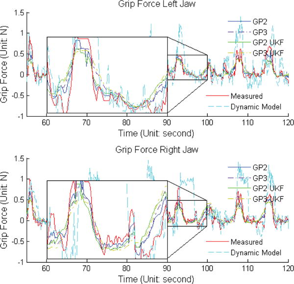
Comparison among Sensor Measured Force and estimation results from the four proposed method and the dynamic model based method.
The difference between the sensor measurements and the estimation results from the four proposed methods and the dynamic model based method were compared with measured gripping force (red line) in Fig. 7. This was to show if the proposed filters caused delay on estimation results and to visualize where the maximum estimation error occurred. Unlike the dynamic model based method, GPR based methods did not have clear delay, even when UKF was adopted. But GPR based UKF (GP2UKF and GP3UKF) were conservative on estimation in the sense that the maximum estimation errors were always around the peak of measured forces. Please notice as the sensor measurements were compared with estimation errors, the y-axis in Fig. 6 and Fig. 7 share the same order.
Fig. 7.
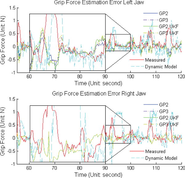
Sensor Measurement and Estimation Error Comparison. Ground truth (sensor measurements) is shown with force estimation errors. Vertical axis label for the red line is Grip Force and for rest of the lines, vertical axis is force error.
The statistical results, including averaged, 99th percentile, and maximum differences, as well as the standard deviation, are shown in Table II. These results shown that the proposed methods had good precision of gripping force estimation and outperformed the dynamic model based method[16], even though no extra sensor or equipment was used.
Table II.
Estimation Error Comparison.
| Averaged (Unit:N) |
SD (Unit:N) |
99%Value (Unit:N) |
Max (Unit:N) |
||
|---|---|---|---|---|---|
| Dynamic | Left | 0.19 | 0.20 | 0.66 | 1.06 |
| Model | Right | 0.28 | 0.30 | 0.86 | 1.15 |
|
| |||||
| GP2 | Left | 0.07 | 0.10 | 0.23 | 0.46 |
| Right | 0.07 | 0.11 | 0.22 | 0.56 | |
|
| |||||
| GP3 | Left | 0.10 | 0.14 | 0.32 | 0.53 |
| Right | 0.10 | 0.13 | 0.26 | 0.54 | |
|
| |||||
| GP2UKF | Left | 0.11 | 0.14 | 0.31 | 0.52 |
| Right | 0.11 | 0.15 | 0.29 | 0.56 | |
|
| |||||
| GP3UKF | Left | 0.12 | 0.17 | 0.38 | 0.63 |
| Right | 0.13 | 0.16 | 0.32 | 0.54 | |
Note: SD: Standard Deviation; 99%value: the threshold of 99% of data
One of the advantages of Gaussian Process Regression is it naturally generates uncertainty estimation. This is especially important to surgical force estimation since safety is the top priority in surgeries. All estimation results and uncertainties were compared with sensor measurements in Fig. 8 and Fig. 9. In the figures, the gray area shown the 99% confidence (3×standard deviation) and the green lines shown the estimation. The uncertainties estimated by the proposed methods are comparatively high, which suggested that in our experiments, the data repeatability is low. In another word, different gripping forces are associated with similar input torque, motor position and velocity. This indicates the selected feature spaces do not have enough resolution for pattern recognition. Fine tuning the robot to make sure its tension, friction condition and other factors may decrease the uncertainties, however, it is difficult.
Fig. 8.
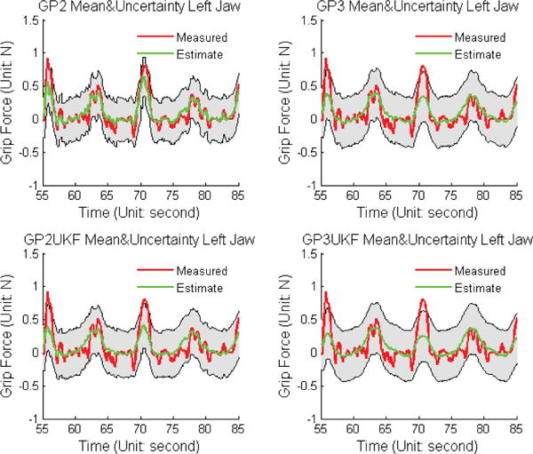
Sensor Measurement and GPR Mean and Uncertainty Comparison for Left Jaw.
Fig. 9.
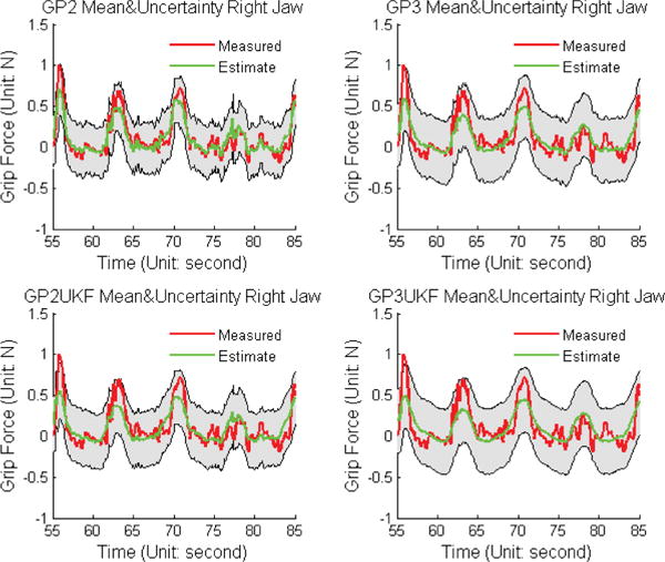
Sensor Measurement and GPR Mean and Uncertainty Comparison for Right Jaw.
The histograms of χ2 errors of the four proposed methods were compared with the χ2 distribution to show if the mean and uncertainty really follow the normal distribution or not, and also to show how the errors are distributed (Fig. 10 and 11). From these figure we can see the estimation results from the four proposed method follow the corresponding χ2, which is a sign indicating good robustness. The numerical difference between the χ2 errors and the corresponding χ2 distribution were compared in Table. III. From the table we can see, agreeing with the precision results, the GP2 has the best similarity between the histogram and the distribution.
Fig. 10.
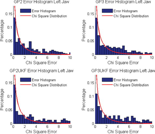
χ2 Error and Distribution Comparison for Left Jaw Force Estimation. The similarity between the histogram and the curve showd the precision of uncertainty estimation.
Table III.
χ2 ERROR AND DISTRIBUTION NUMERICAL COMPARISON.
| GP2 | GP3 | GP2UKF | GP3UKF | |
|---|---|---|---|---|
|
| ||||
| left | 0.02 | 0.02 | 0.02 | 0.02 |
| right | 0.02 | 0.02 | 0.02 | 0.03 |
C. Analysis and Discussion
The experimental results demonstrated that the Gaussian Process Regression estimators outperformed the dynamic model base UKF estimator on precision for the sensorless gripping force estimation problem, which suggests that GPR suits our application. The GPR estimators proposed in the paper also provided uncertainty estimation as a side product, which would be useful because we will fuse force estimation results from multiple sources to further improve estimation precision and stability in our future work.
Table II indicated that among all four estimators, GP2 had the best force and uncertainty estimation. If we take a closer look at Fig. 6, 7, 8 and 9 we can find that GPR based UKF estimators tended to be more “conservative” than the GPR estimators, as they generated smoother estimations, which also caused the force peak values to be far away from the sensor measurements. In teleoperated surgical systems, the smoothness may be preferable because it increases the systematic stability. However, Fig. 10 and 11 demonstrated that the smooth estimations from GP2UKF and GP3UKF have less similarity to the χ2 distribution, which indicated the inconsistency between the mean and uncertainty estimation.
Experimental results also shown that, although the precision difference between GP2 and GP3, and between GP2UKF and GP3UKF are not huge, GP2 and GP2UKF were still slightly better. It is possible that this is due to the fact that the velocity estimation from position observations not only probabilistically depended on the position observation, but also introduced extra delay since we adopted a causal low pass filter. However, it may also suggest that GPR had very strong power to overcome the nonlinearity.
The computational complexity of GPR was thoroughly analyzed in [17]. In the proposed methods, the estimators trained with hundreds of data points, which made the computational complexity trivial to modern computers. As for the proposed estimators, it was clear GP3UKF had highest computational complexity, and GP2UKF was higher than GP3, while GP2 had the lowest complexity.
V. Conclusion
GPR based estimators were proposed to address the sensorless gripping force estimation problem for elongated cable driven surgical instruments. Compared to explicitly modeling the system, GPR has the advantages that it learns from data, is simple, and naturally generates estimation uncertainties. The four estimators were proposed and designed based on our study of surgical instrument properties and cable characterization. The proposed methods were compared with the dynamic model based estimator on a 10mm gripper on the Raven II surgical robot. Experimental results demonstrated that the GPR estimators outperformed the dynamic model based estimator in the application, and among the four estimators, the simplest, GP2, had the best estimation precision and reliability. The results suggested that the proposed GPR with 2-dimensional inputs best fitted our application.
Next, the proposed method needs to be combined with teleoperation consoles to close the haptic feedback loop and to verify that the technique meets clinical needs. We also need to explore the usage of long-term learning[26] to improve the adaptiveness of the proposed method. Moreover, combining the GP2 estimator with other force estimation techniques, such as estimations of contacted tissue deformation, also attracts us. These extra information may be able to form a better feature space and achieve higher estimation precision and reliability. We also have the option to directly combine the GPR estimation results with those estimation techniques, through utilizing the uncertainty estimation of GPR and further improve estimation precision and reliability.
Acknowledgments
*This work was supported by NIH grant 5R21EB016122-02, NSF grant 1227406 and the Korean Institute of Science and Technology (KIST, Dr. Hujoon project).
Footnotes
This paper was recommended for publication by Editor Ken Masamune upon evaluation of the Associate Editor and Reviewers’ comments.
References
- 1.Mack MJ. Minimally invasive and robotic surgery. Jama. 2001;285(5):568–572. doi: 10.1001/jama.285.5.568. [DOI] [PubMed] [Google Scholar]
- 2.Gomes P. Surgical robotics: Reviewing the past, analysing the present, imagining the future. Robotics and Computer-Integrated Manufacturing. 2011;27(2):261–266. [Google Scholar]
- 3.Puangmali P, Althoefer K, Seneviratne LD, Murphy D, Das-gupta P. State-of-the-art in force and tactile sensing for minimally invasive surgery. Sensors Journal, IEEE. 2008;8(4):371–381. [Google Scholar]
- 4.Hammond FL, Kramer RK, Wan Q, Howe RD, Wood RJ. Soft tactile sensor arrays for force feedback in micromanipulation. Sensors Journal, IEEE. 2014;14(5):1443–1452. [Google Scholar]
- 5.Prasad SK, Kitagawa M, Fischer GS, Zand J, Talamini MA, Taylor RH, Okamura AM. A modular 2-dof force-sensing instrument for laparoscopic surgery. in Medical Image Computing and Computer-Assisted Intervention-MICCAI 2003 Springer. 2003:279–286. [Google Scholar]
- 6.Vatani M, Engeberg ED, Choi J-W. Force and slip detection with direct-write compliant tactile sensors using multi-walled carbon nanotube/polymer composites. Sensors and Actuators A: physical. 2013;195:90–97. [Google Scholar]
- 7.Tholey G, Pillarisetti A, Green W, Desai JP. Design, development, and testing of an automated laparoscopic grasper with 3-d force measurement capability. in Medical Simulation Springer. 2004:38–48. [Google Scholar]
- 8.Katsura S, Matsumoto Y, Ohnishi K. Modeling of force sensing and validation of disturbance observer for force control. Industrial Electronics, IEEE Transactions on. 2007;54(1):530–538. [Google Scholar]
- 9.Zhao B NC. Estimating tooltissue forces using a 3-degree-of-freedom robotic surgical tool. ASME J Mechanisms Robotics. 2016;8(5) doi: 10.1115/1.4032591. [DOI] [PMC free article] [PubMed] [Google Scholar]
- 10.Khoshnam M, Skanes AC, Patel RV. Modeling and estimation of tip contact force for steerable ablation catheters. IEEE Transactions on Biomedical Engineering. 2015;62(5):1404–1415. doi: 10.1109/TBME.2015.2389615. [DOI] [PubMed] [Google Scholar]
- 11.Berger E. Friction modeling for dynamic system simulation. Applied Mechanics Reviews. 2002;55(6):535–577. [Google Scholar]
- 12.Anooshahpour F, Polushin IG, Patel RV. Quasi-static modeling of the da vinci instrument. in Intelligent Robots and Systems (IROS 2014), 2014 IEEE/RSJ International Conference on IEEE. 2014:1308–1313. [Google Scholar]
- 13.Townsend WT. PhD dissertation. MIT; Cambridge, MA: 1988. The effect of transmission design on force-controlled manipulator performance. [Google Scholar]
- 14.Miyasaka M, Haghighipanah M, Li Y, Hannaford B. Hysteresis model of longitudinally loaded cable for cable drivenrobots and identification of the parameters. in Robotics and Automation, 2016 ICRA ’16 IEEE International Conference on. 2016 doi: 10.1109/icra.2016.7487605. [DOI] [PMC free article] [PubMed] [Google Scholar]
- 15.Muneaki Miyasaka AL, Matheson Joseph, Hannaford B. Int Conf on Intelligent Robots and Systems (IROS) Hamburg, German: Oct, 2015. Measurement of the cable-pulley coulomb and viscous friction for acable-driven surgical robotic system. [Google Scholar]
- 16.Li Y, Miyasaka M, Haghighipanah M, Cheng L, Hannaford B. Dynamic modeling of cable driven elongated surgical instruments forsensorless grip force estimation. Robotics and Automation, 2016 ICRA ’16 IEEE International Conference on. 2016 doi: 10.1109/icra.2016.7487605. [DOI] [PMC free article] [PubMed] [Google Scholar]
- 17.Rasmussen CE. Gaussian processes for machine learning. 2006 [Google Scholar]
- 18.Hannaford B, Rosen J, Friedman DW, King H, Roan P, Cheng L, Glozman D, Ma J, Kosari SN, White L. Raven-ii: an open platform for surgical robotics research. Biomedical Engineering, IEEE Transactions on. 2013;60(4):954–959. doi: 10.1109/TBME.2012.2228858. [DOI] [PubMed] [Google Scholar]
- 19.Bishop CM. Pattern recognition. Machine Learning. 2006;128 [Google Scholar]
- 20.Wan EA, Van Der Merwe R. Adaptive Systems for Signal Processing, Communications, and Control Symposium 2000 AS-SPCC The IEEE 2000. Ieee; 2000. The unscented kalman filter for nonlinear estimation; pp. 153–158. [Google Scholar]
- 21.Manchester IR, Slotine J-JE. in Control Conference (AUCC), 2014 4th Australian. IEEE; 2014. Output-feedback control of nonlinear systems using control contraction metrics and convex optimization; pp. 215–220. [Google Scholar]
- 22.Haghighipanah M, Miyasaka M, Li Y, Hannaford B. 2016 IEEE International Conference on Robotics and Automation (ICRA) IEEE; 2016. Unscented kalman filter and 3d vision to improve cable driven surgical robot joint angle estimation; pp. 4135–4142. [DOI] [PMC free article] [PubMed] [Google Scholar]
- 23.Ko J, Klein DJ, Fox D, Haehnel D. Gp-ukf: Unscented kalman filters with gaussian process prediction and observation models. Intelligent Robots and Systems, 2007 IROS 2007 IEEE/RSJ International Conference on IEEE. 2007:1901–1907. [Google Scholar]
- 24.Cheng L. Ph D dissertation. 2015. Computation and measurement of force and tissue damage for the grasper-tissue interface in robot-assisted minimal invasive surgery. [Google Scholar]
- 25.Li Y, Olson EB. Extracting general-purpose features from lidar data. in Robotics and Automation (ICRA), 2010 IEEE International Conference on IEEE. 2010:1388–1393. [Google Scholar]
- 26.Deisenroth MP, Fox D, Rasmussen CE. Gaussian processes for data-efficient learning in robotics and control. Pattern Analysis and Machine Intelligence, IEEE Transactions on. 2015;37(2):408–423. doi: 10.1109/TPAMI.2013.218. [DOI] [PubMed] [Google Scholar]


