Abstract
Computed tomography laser mammography (Eid et al. Egyp J Radiol Nucl Med, 37(1): p. 633–643, 1) is a non-invasive imaging modality for breast cancer diagnosis, which is time-consuming and challenging for the radiologist to interpret the images. Some issues have increased the missed diagnosis of radiologists in visual manner assessment in CTLM images, such as technical reasons which are related to imaging quality and human error due to the structural complexity in appearance. The purpose of this study is to develop a computer-aided diagnosis framework to enhance the performance of radiologist in the interpretation of CTLM images. The proposed CAD system contains three main stages including segmentation of volume of interest (VOI), feature extraction and classification. A 3D Fuzzy segmentation technique has been implemented to extract the VOI. The shape and texture of angiogenesis in CTLM images are significant characteristics to differentiate malignancy or benign lesions. The 3D compactness features and 3D Grey Level Co-occurrence matrix (GLCM) have been extracted from VOIs. Multilayer perceptron neural network (MLPNN) pattern recognition has developed for classification of the normal and abnormal lesion in CTLM images. The performance of the proposed CAD system has been measured with different metrics including accuracy, sensitivity, and specificity and area under receiver operative characteristics (AROC), which are 95.2, 92.4, 98.1, and 0.98%, respectively.
Keywords: Breast cancer, Computed tomography laser mammography (CTLM), Computer-aided diagnosis systems (CADs), 3D shape features, 3D GLCM features, Multi-layer perceptron neural network (MLPNN)
Introduction
Breast cancer is the most prevalent cancer that affects women all over the world. Early detection and diagnosis of breast cancer play a significant role to reduce the mortality rate as well as to increase the prognosis of patients. Mammography is the golden standard for breast imaging. Breast screening with mammography involves passing radiation (X-ray) through the breast. Evidence indicates the growth of risk of breast cancer with exposure to multiple mammographies, especially in women with genetic predisposition due to impaired deoxyribonucleic acid (DNA) repair mechanisms [2]. The results show that the sensitivity in women with fatty breast is roughly 88% but drastically decreased in women with dense breast which is 62% [3]. On top of that, the risk of developing breast cancer in dense breasts is four to six times higher than in non-dense breasts [4].
In recent years, several studies have been conducted to find alternative methods to adjunct mammography in order to enhance sensitivity and specificity. Computed tomography laser mammography (CTLM) is an optical imaging technique which is presented for breast screening, particularly in women under the age of 40 and who have dense breasts. CTLM is a non-invasive and cost-effective modality that uses near-infrared light propagation through the tissue to assess its optical properties. Different tissue components have unique scattering and absorption characteristics for each wavelength. In new forming tumours, the blood flow increases and the CTLM then looks for high haemoglobin concentration (angiogenesis) in the breast to detect neovascularization, which may be hidden in mammography images, especially in dense breast [1, 5, 6]. Malignant lesions will be detected based on their higher optical attenuation compared to the surrounding tissue, which is mainly related to the increase in light absorption by their higher haemoglobin content [7].
CTLM image interpretation is not an easy task due to the shape diversity of angiogenesis [6]; thus, a radiologist is required to have specific skills to interpret and distinguish between normal veins and abnormal angiogenesis. Analysis of CTLM image is based on the absorption pattern of haemoglobin in vessels. Bright areas indicate the aggressiveness of cancer, while angiogenesis can appear in any shade of green. The detection of angiogenesis in CTLM images does not only rely on the brightness but also on the various abnormality shapes and volumes [8]. The radiologist needs to explore in a 2D plane to find any bright green areas that show distortion or deviation and investigates the irregular shape of angiogenesis in 3D view [8].
Generally, in clinical imaging assessment, some issues affect the interpretation of radiologists such as technical reasons which are related to imaging quality [9] and human error [10] due to the structural complexity in appearance. Computer-aided detection/diagnosis (CAD) systems have been developed for automatic detection and classification of the suspicious area on different modality. CAD systems help the radiologist in the interpretation of medical images to detect and differentiate between benign and malignant lesions. CAD systems are used as a double reader for accuracy enhancement and final decision which is made by the physician.
The fact that diagnosis in CTLM images for a radiologist is time-consuming and complicated due to a variety of angiogenesis shape [6]; thus, an automatic system to detect and classify abnormality is desirable. It is expected that the efficiency and effectiveness of diagnosis can be increased by CTLM-CAD system. The purpose of this study is to develop a computer-aided detection/diagnosis (CAD) system in CTLM that would act as the radiologist assistant in order to reduce misdiagnosis as well as to differentiate between normal and abnormal tissue within the breast.
Related Works
Computed tomography laser mammography is a new optical imaging modality for breast cancer detection [8, 11]. Major advantages of optical imaging techniques do not include the use of any ionising as mammography or any radioactive components as positron emission tomography (PET), and it is relatively economical [12]. In the most modalities, breast density is a significant agent which has impacted the cancer diagnosis. As a striking feature, the CTLM’s laser is not impeded by dense breast [8, 11, 13]. CTLM use near infrared (NIR) laser light in a specific wavelength (808 nm) that can be absorbed by blood and able to visualise neovascularisation [14]. During the CTLM imaging procedure, the scanning mechanism transmits laser light by rotating 360° starting from the chest wall to the breast. Part of the light is absorbed by tumour or blood vessels, and the remaining part is registered by the detector. The area with high haemoglobin concentration (neo-angiogenesis) contains more absorption. After complete rotation, the scanning mechanism will automatically descend to a predetermined distance to register the next slice data [6]. The slice thickness is adjusted to 2–4 mm in accordance with the breast size. This process is repeated to the nipple area as well as to scanning the whole breast.
Optical imaging foundation is presented in Fig. 1, in which a tumour with high haemoglobin concentration is observed in Fig. 1a. The laser lights that pass through the breast are absorbed by the neo-angiogenesis area as shown in Fig. 1b, and the remaining lights will be recorded by the detector as shown in Fig. 1c.
Fig. 1.
Optical imaging foundation [15]
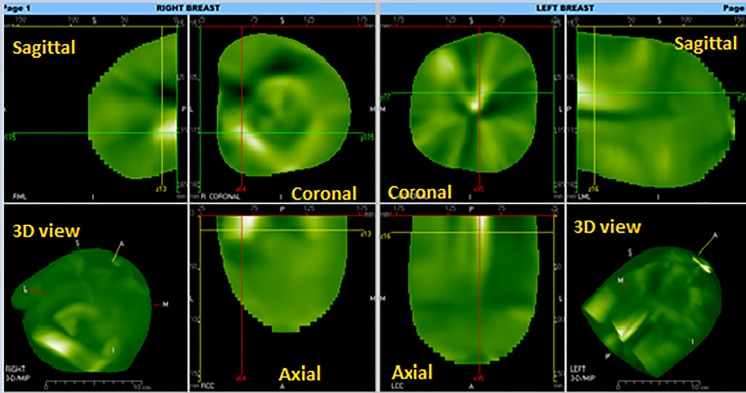
The diffusion approximation of transport (Eq. [16]) is used to reconstruct CTLM images slice by slice. The CTLM workstation is capable of displaying it in three planes, namely sagittal, axial and coronal (2D) as well as a 3D view of the whole breast as shown in Fig. 2. CTLM interpretation is based on the absorption pattern of haemoglobin in the vessels. The detection of angiogenesis in CTLM images does not only rely on the brightness but is also required to recognise various abnormality in shapes and volumes [8]. Bright areas indicate aggressiveness of cancer, while angiogenesis can appear in any shade of green. Normal vessels are tubular and ribbon shape, which gets bigger from the nipple to the chest wall. This ribbon can be seen in axial and sagittal views. Coronal images demonstrate lobular blood supply that is in wedge-shaped, which is also broad on the skin and the apex towards the centre. Any distortion and deviation in sagittal and coronal views can be considered an abnormality.
Fig. 2.
The 2D and 3D image in CTLM workstation
In 3D space, the images are analysed in two different projections, namely maximum intensity projection (MIP) and front to back projection (FTB) [17]. FTB mode improves the quality of the image and presents the significant parts of the image by applying surface rendering using window/level adjustment. Angiogenesis occurs only in deep veins and not in superficial vessels, and it can appear in irregular 3D shapes such as an oblate sphere, a dumbbell shape, diverticulum, circle and free standing [8].
The radiologist needs to explore in the 2D planes for any bright green areas that show distortion or deviation and investigate the irregular shape of angiogenesis in 3D view [8]. In the first step of conventional way CTLM image interpretation, radiologists look at the 2D views of sagittal and coronal views to find any distortion and deviation in different slices. If any abnormality is detected in coronal or sagittal views, the next step will be performed for more investigation in 3D space. The results of surface rendering are highly dependent on the amount of window and level values selected by a radiologist. The outcomes of surface rendering in FTB mode can be rotated to explore different shapes of angiogenesis. The radiologist performs localisation of abnormality based on clock face quadrant and lateral view for prior, mid-segment and posterior.
Materials and Methods
Experimental Dataset
In this study, the CTLM breast images of women have been acquired from clinical screening in Breast Wellness Centre, Malaysia, and two datasets of Medoc centre in Budapest, Hungary, and TATA Hospital in Mumbai, India. The distribution of breast density does not affect the sensitivity and specificity of the study [8, 11, 13]. This dataset includes CTLM images, also ultrasound and mammography images to correlate cancerous area in CTLM images with ultrasound and mammography images. The collected data have been released on the website (http://www.upm-ctlmimages.net/). A total of 180 patients have been examined with CTLM and ultrasound for patients under the age of 40, while CTLM, ultrasound and mammography were conducted for those above the age of 40. A total of 48 cases have been reported as malignant by two expert radiologists and correlation of ultrasound and mammography images. The study was approved by the local Ethics Committee (Universiti Putra Malaysia - Ethics reference number UPM/TNCPI/RMC/1.4.18.1 (JKEUPM)/F2), and written informed consent was obtained from all patients.
Analysis of CTLM Images with the CAD System
The development of an effective computer-aided diagnosis for breast cancer possesses significant clinical importance in raising the survival rate of the patients. CTLM is a non-invasive imaging modality for breast cancer diagnosis, which is time-consuming and challenging for the radiologist to interpret the image. Some studies have indicated that CTLM may provide additional information to characterise benign and malignant lesions when adjunct to other breast screening [8, 17]. The general objective of this study is to develop a computer-aided diagnosis framework in order to enhance the performance of radiologist in the interpretation of CTLM images.
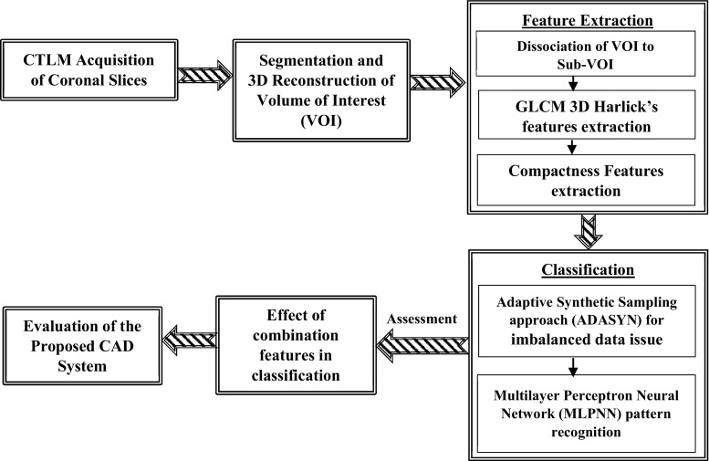
The foundation of the proposed CAD system has shown in Fig. 3 for detection of abnormality in the CTLM images. The first step of CAD system is to design a fully automatic 3D segmentation and reconstruction technique to elicit volume of interests (VOIs) from a background of CTLM image. A 3D Fuzzy segmentation technique has been implemented to extract the volume of interest (VOI). The extracted VOIs from CTLM image is a connected area which needs to split into sub-VOIs before feature extraction. The dissociation model has been proposed to split VOIs based on the centroid of 2D objects. The shape and texture of angiogenesis in CTLM images are significant characteristics to differentiate malignancy or benign lesions. The 3D compactness features and 3D grey level co-occurrence matrix (GLCM) have been extracted to achieve the second objective. Classification of imbalanced distributed data degrades the prediction accuracy of the most standard machine learning techniques. This study focuses on binary classification for breast cancer detection on the CTLM dataset which include 180 patients in which a total of 132 instances are labelled with normal and the remaining 48 are labelled abnormal, based on two expert radiologist reporting and correlation with their mammography and ultrasound images. After dissociated VOIs to sub-VOIs, the number of negative instance in our dataset is much higher than positive instances which reflect the imbalanced class distribution. To obviate the class imbalance problem, ADASYN oversampling techniques are used to balance the number of positive and negative instances. Multilayer perceptron neural network (MLPNN) pattern recognition has developed for classification of the normal and abnormal lesion in CTLM images. The effect of the different combination of 3D shape and GLCM features on the accuracy of classifier have been evaluated to achieve the best combination features to diagnosis abnormality in the CTLM images.
Fig. 3.
Proposed CAD system for breast cancer detection in CTLM images
3D Segmentation of Volume of Interests from CTLM Background
Segmentation is a critical step in CAD systems conducted by extracting substantial anatomical structures from a background of images. CTLM is a 3D imaging modality that serves to provide specific information in order to analyse vascular anatomy in the breast. The 3D shapes of neo-angiogenesis which represent the cancer growth are very important in the diagnosis of breast cancer in CTLM images. The 2D segmentation techniques are not capable of displaying different forms of angiogenesis in CTLM images; therefore, the 3D automatic segmentation techniques are of great interest in the segmentation of CTLM images. The three automatic segmentation techniques include Fuzzy C-means clustering (FCM), K-mean clustering and colour quantization method [18] and have been implemented in our previous study [19, 20] to extract volume of interest from CTLM images. In order to accept the segmentation results in clinical practice, the quantitative evaluation is crucially important. The challenging task in quantitative evaluation is finding the ground truth for the evaluation segmentation results. In the field of radiology, window width and window level are used to establish ground truth images to assess the accuracy of segmentation algorithm [21]. This feature is used by the radiologists to review CTLM images in conventional diagnosis. The windows/level values adjusted by radiologists in manual diagnosis are utilised to extract the ground truth in our work. The values can vary from one patient to another based on the structure preferred by the radiologist in the surface rendering of the CTLM image.
Due to the impact of segmentation in subsequent stage as classification, the evaluation of segmentation methods has special significance in the medical imaging field. To date, there are no desirable segmentation methods that can provide satisfactory results in all medical imaging modalities. To find the most appropriate segmentation method in a specific issue, it needs to be decided experimentally. In order to accept the segmentation results in clinical practice, the quantitative evaluation is crucially important. Among the number of the region-based coefficients, the Jaccard [22] and Dice [23] coefficients have been widely used for performance evaluation of the segmentation methods in clinical imaging. These coefficients’ measure is calculated with true positive, false positive and false negative values. If G is the set of voxels in ground truth image and S is the set of voxels in segmented image, TP is the number of voxels in the intersection of G and S, while FP is the number of voxels in G that does not belong to S, and FN is the number of voxel in S and does not belong in G.
| 1 |
| 2 |
The ratio of volumetric overlap error [24] can also be assessed by Eq. (3).
| 3 |
The value varies between 0 and 100 and zero value signifies perfect segmentation.
Dissociation Object Model on VOIs and Feature Extraction
Feature extraction is the next stage of the proposed CAD system to exploit the significant characteristics of VOIs. In CTLM image segmentation, the extracted volume may consist of normal blood vessels or neo-angiogenesis which is a sign of tumour growth. The extracted VOIs from CTLM image are connected areas that need to be split into sub-VOIs before feature extraction. A dissociation model has been proposed to split VOIs based on 2D region properties of image objects based on the centroid of 2D objects. Each object in the 2D images has many region properties such as area, bounding box, centroid, convex hull, eccentricity, extrema and many more features. Figure 4a, b shows the segmented objects in the 2D slice, and Fig. 4c shows the segmented objects in sequential slices which are highlighted with orange colour.
Fig. 4.
View of region properties in sequential slices. a Centroid of an object in a 2D slice. b Segmented objects in a 2D slice. c Centroid of objects in sequential slices
The 2D segmented CTLM image contains one or more objects. If X and Y show the centroid of objects in consecutive slices, the Euclidean distance of each object is calculated with all objects in the next slice. Since the irregular forms of angiogenesis are shown in the oblate sphere, diverticulum, dumbbell shaped [8], the displacement of object centroid can indicate diversion of blood vessels to the tumour. The displacement of centroid among two objects in sequential slices is obtained by Euclidian distance Eq. (4). At this point, a threshold value is required if the displacement of two centres is less than the threshold, which shows that the deviation of the object is less than the specified amount. Hence, two objects are connected to each other or otherwise further objects are examined. Since 1 mm = 3.779527559 pixels, the threshold value is considered to be related to the number of pixels in the image. In this work, an arbitrary value use for the threshold is between 15 and 30 pixels (displacement value ≈4–8 mm), and the trial and error method is applied to determine which threshold value performs the desirable dissociation of VOIs.
| 4 |
The probability of malignancy in CTLM image depends on the shape and texture of lesions; thus, the diagnosis tasks are designed to extract corresponding features based on these characteristics. These features can be categorised into texture features and morphological features [25]. With the development of 3D imaging modalities, demands have been increasing for 3D feature descriptors to raise the performance of the classifier. The texture is one of the most prevalent features that are used to analyse and interpret images, specifically in clinical imaging. The variation of the surface intensity and several attributes such as smoothness, coarseness and regularity have to be measured through the texture [26]. The texture of biomedical image can be used to describe the suspected regions by the training of existing samples to learn the distinctive patterns associated with normal and abnormal tissues [27]. In this study, textural features have been extracted to differentiate the characteristics of a normal and abnormal tissue in CTLM images.
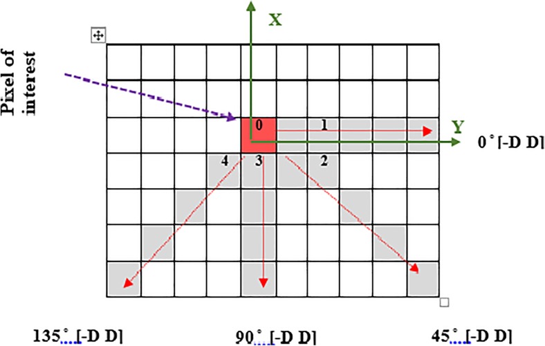
Among the various texture computation techniques presented, Halick [28] is the most prevalent method for textural feature extraction in a different application specifically in clinical imaging. The traditional 2D co-occurrence matrices are used to capture spatial dependence of the grey levels value of pixel pairs within certain angles and distances. The GLCM has used an array of offsets to determine pixels relationship in distinct direction and distance to the creation of GLCM matrices. Figure 5 shows the spatial relationship of pixels in four directions and distances which represent the input image by 16 GLCMs. The red pixel considers as coordinate (0, 0) and the offsets show the direction relative to the axis.
Fig. 5.
Spatial relationship of pixels and offset of neighbours (2D space). Offset 1 = (0 1), Offset 2 = (−1 1), Offset 3 = (−1 0) and Offset 4 = (−1 −1)
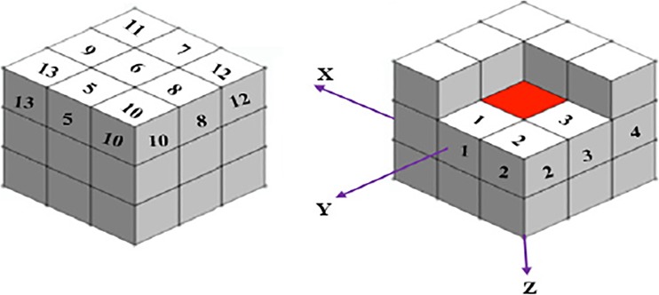
With recent advances in technology particularly in medicine, new types of data with volumetric properties have emerged. The 2D GLCM extraction techniques are not able to extract the 3D texture characteristics of the volumetric data. To address this issue, 2D GLCM extraction techniques are spread to the 3D GLCM texture features. Based on the theory of 2D GLCM, the concepts and structure of 3D GLCM are shown in Fig. 6. In a 3D matrix of pixels (3 × 3 × 3), assume that the centre point (red colour) is the intersection of the three axes X, Y and Z. The centroid pixel has 26 nearest neighbours leading to 26 different directions. Each direction and its opposite have the same co-occurrence matrix [29]; thus, we have considered only 13 directions as shown in Fig. 6. In this study, the values considered for the distances of voxel which included 1, 2, 4 and 8. Therefore, four different values of distance and 13 directions obtained by 52 GLCM matrices are used. A total of 12 Harlick’s feature [28] are calculated from 3D GLCM matrices which consist of energy, entropy, correlation, contrast, variance, sum means, inertia, cluster shade, cluster tendency, homogeneity, max probability and inverse variance. In order to reduce the dimension of extracted features, the mean value of Harlick’s features for the same distance has been calculated in different directions. Therefore, for each Harlick’s feature, four different values and a total of 48 GLCM texture features are obtained. The formulas and a brief description of the Harlick’s features with respect to the texture characterisation are presented in Table 1 [26, 30–33].
Fig. 6.
Spatial relationship of pixels and offset of neighbours (3D space) Offset 1 = (0 1 0), Offset 2 = (−1 1 0), Offset 3 = (−1 0 0), Offset 4 = (−1 −1 0), Offset 5 = (0 1 −1), Offset 6 = (0 0 −1), Offset 7 = (0 −1 −1), Offset 8 = (−1 0 −1), Offset 9 = (1 0 −1), Offset 10 = (−1 1 −1), Offset 11 = (1 −1 −1), Offset 12 = (−1 −1 −1) and Offset 13 = (1 1 −1)
Table 1.
The Harlick’s texture feature from GLCM
| Feature | Formula | Description |
|---|---|---|
| Energy (angular second moment) | Measure the local homogeneity and, therefore, show the opposite of the entropy. The energy value is high with the larger homogeneity of the texture. | |
| Entropy | Measure the randomness of a grey-level distribution. The Entropy is expected to be high if the grey-levels are distributed randomly through the image. | |
| Correlation | Measure the joint probability occurrence of the certain pixel pairs. The correlation is expected to be high if the grey levels of the pixel pairs are highly correlated. | |
| Contrast | Measure the local variations in the grey level co-occurrence matrix. The contrast is expected to be low if the grey levels of each pixel pair are similar. High contrast values are expected for heavy textures and low for smooth, soft textures | |
| Variance | Variance shows how is spread out the distribution of grey levels. The variance is expected to be large if grey levels of image are spread out greatly | |
| Sum mean (Mean) | Presents the mean of the grey levels in the image. The sum mean is expected to be large if the sum of the grey levels of the image is high. | |
| Inertia (second difference moment) | Inertia is very sensitive to large variation in GLCM. It is expected to be high in highly contrast regions and low for homogeneous regions. | |
| Cluster Shade | Measure the skewness of GLCM and represent the perceptual concepts of uniformity. It expected to be high in the asymmetric image. | |
| Cluster Tendency | Measure the grouping of pixels that have similar grey levels. | |
| Homogeneity | Measures the uniformity of non-zero entry and closeness of the distribution of elements in GLCM. The homogeneity is expected to be high if GLCM concentrates along the diagonal. | |
| Max Probability (MP) | Results the pixel pair that is most predominant in the image. The MP is expected to be high if the occurrence of the most predominant pixel pair is high. | |
| Inverse variance | Also called Inverse Difference Moment, similar to homogeneity. It is expected low for inhomogeneous and high for the homogeneous image. |
The shape of angiogenesis in CTLM images is a significant characteristic to determine malignancy or a benign lesion. As mentioned in “Dissociation Object Model on VOIs and Feature Extraction” section, the normal blood vessels are in tubular and ribbon shape which becomes narrower from the chest wall to the nipple. Haemoglobin concentration (angiogenesis) leads to the emergence of distortion and deviation in the direction of the blood vessels. The deformation of blood vessels in angiogenesis area appears in different shapes such as dumbbell-shaped, diverticulum, freestanding and polypoid [8]. The use of the shape descriptors can be effective in differentiating between the blood vessels and angiogenesis.
Compactness is the inherent properties of an object, which is one of the most common morphological descriptors for shape analysis. Several 3D shape compactness measures have been developed with extends of 2D compactness measure [34–37]. In this study, three different compactness measures are applied as shape descriptor which is presented in continue. The classical compactness of a 3D object is measured by which is dimensionless and minimised by a sphere [37]. Bribiesca [36] proposed a compactness measure by the relation among the area of surface enclosed to the volume and contact area. The proposed measure is invariant under translation, rotation and scaling. The measure of descript compactness C d for a 3D shape composed of n voxel is defined by Eq. (5).
| 5 |
where A C is the contact surface area and A is the area of the enclosing surface.
Another definition of compactness measure is presented by [35] with comparing a shape S with its fit sphere B fit. Assume that S is a shape and a sphere B fit that its centre coincides with the centroid of S with radius . The compactness k fit(S) is shown in Eq. (6).
| 6 |
The other compactness measure developed by [35] is based on the geometric moment [38]. The (p, q, r)-moment of a 3D shape S is defined by Eq. (7).
| 7 |
Assume that S is a sphere which its centroid coincides with the origin and C is a sphere with radius , where μ 0 , 0 , 0 shows the centralised moment. The compactness value based on presented method in [34, 35] is calculated by Eq. (8).
| 8 |
Feature selection is a significant phase in many bioinformatics application due to reducing the storage requirement and reducing the training time of classifier. Generally, feature selection techniques organised into three categories: filter methods, wrapper methods and embedded methods [39, 40]. In this work, the sequential forward selection technique has utilised to choose appropriate features. In addition, a variety of manual categorization of features has been used to assess the performance of the proposed classifier (Table 2).
Table 2.
The different combinations of GLCM 3D and shape features
| No. | Features | Number of features |
|---|---|---|
| 1 | Compactness | 3 |
| 2 | Compactness and energy | 7 |
| 3 | Compactness and entropy | 7 |
| 4 | Compactness and correlation | 7 |
| 5 | Compactness and contrast | 7 |
| 6 | Compactness and variance | 7 |
| 7 | Compactness and Sum mean | 7 |
| 8 | Compactness and inertia | 7 |
| 9 | Compactness and Cluster shade | 7 |
| 10 | Compactness and Cluster tendency | 7 |
| 11 | Compactness and homogeneity | 7 |
| 12 | Compactness and max probability | 7 |
| 13 | Compactness and inverse variance | 7 |
| 14 | GLCM-3D | 48 |
| 15 | Compactness and GLCM-3D | 52 |
| 16 | Selected features with sequential forward selection method (energy, compactness, contrast, inverse variance, cluster shade, homogeneity, inertia, max probability) | 18 |
Classification Technique for Breast Cancer Lesions in CTLM Image
Classification of imbalanced distributed data is the cause of the degrading prediction accuracy of the most standard machine learning techniques. In binary classification, this problem occurs when the number of instances from one class is significantly less than another class. Prediction cost for minority class is higher than the majority class, especially in medical datasets that high-risk patients placed in minority class [41]. The use of imbalanced data in the learning stage will result in high accuracy and sensitivity, while the specificity value will be low.
This study focuses on binary classification for breast cancer detection on CTLM dataset. Based on the two expert radiologists report and correlation with their mammography and ultrasound images, the CTLM dataset obtained from 180 patients with a total of 132 instances labelled normal and the remaining 48 labelled abnormal. The proposed dissociation model divides the segmented VOIs into sub-VOIs (5–10 objects for each image). In breast cancer patients, one or two sub-VOIs are labelled as positive. Therefore, the number of negative instances is too much higher than the positive instances which reflect imbalanced class distribution.
Selecting an appropriate sampling technique is an additional procedure to improve the classifier performance. The minority instances are of great importance in machine learning techniques to achieve high performance of classification. Adaptive synthetic (ADASYN) sampling approach is an oversampling method which is used in this work [42]. The main idea of ADASYN method is the weight distribution for a minority class to commensurate with the degree of difficulty in learning. In this method, more synthetic data are produced for the minority instances which are more complex to learn than other minority instances. The ADASYN method improves learning with respect to the data distribution in two ways: (1) reducing the bias provided by imbalanced classes and (2) shifting the classification decision boundary adaptively towards the complex samples [42]. The positive instances generated by ADASYN repeatedly add to multiple mini-batches to avoid the overfitting issue [43]. The balance level β in ADASYN method has been adjusted to 1 on training data to represent the fully balanced dataset. The number of synthetic samples that is required to be generated for each minority instance is defined based on their density distribution (). The is a measure of the distribution weight for each minority instance proportional to their complexity in learning. Therefore, ADASYN concentrates more on difficult instances to learn by shifting the classifier boundary.
The variety of features set includes texture and shape features which are described in “Analysis of CTLM Images with the CAD System” section and have been extracted from sub-VOIs. These features include three different compactness features and 12 Harlick’s features GLCM 3D. With reference to “Analysis of CTLM Images with the CAD System” section, the Harlick’s features are extracted in four different directions. Therefore, each Harlick’s features contains four values and the combination with compactness features includes seven features. The total number of GLCM 3D features is 48, and the overall number of compactness and GLCM 3D features is 52. These features are extracted from centroid-based object dissociation model (CODM). The different combinations of Harlick’s features GLCM 3D and compactness contain 16 groups of features which are shown in Table 2. The feature groups F1–F15 are various combination of compactness features and the Harlick’s features, and group feature F16 is the selected features by sequential forward selection method. The different categories of features (Table 2) are used to train and test in the proposed multilayer perceptron neural network (MLPNN) pattern recognition. The overview of our experimental design for MLPNN classification is shown in Fig. 7.
Fig. 7.

The overview of proposed experimental design on MLPNN classification
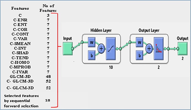
Multilayer perceptron (MLP) is a feed forward neural network model which is widely used in analysing the object characteristics in order to recognise the patterns. Matlab neural network toolbox is an interactive environment that provides a suitable context for the implementation of a neural network for clustering, fitting, pattern recognition and time series. The MLP neural network is a supervised method that uses a pair of {X, L}, where X is a set of extracted features and L is the label of the corresponding object. In this study, an MLP classification method is designed to classify normal and abnormal objects in CTLM image for the diagnosis of breast cancer. To obtain the appropriate number of the hidden layer, the performance of the proposed MLPNN is evaluated by the different number of hidden layer (Fig. 12). Increasing the number of hidden layers does not significantly affect the performance of MLPNN and leads to the increase of learning time. Therefore, a number of the hidden layers has been considered as ten for further experiments. The output layer represents the outcome of the neural network over the activation pattern applied to the input layer, in which the proposed MLPNN contains two neurones to produce a binary classifier.
Fig. 12.
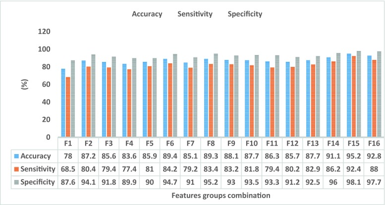
Performance of the proposed MLPNN classifier with different combination of features
The balanced data with ADASYN oversampling is used to train the neural network. Seventy per cent of input data are used for training, 15% for testing and the rest of the data (15%) for validation. A loop is embedded in the training procedure to improve learning performance, and the condition for exiting the loop is intended based on training error. If the training error is below 5% learning end, the loop is then repeated 50 times. The features are separately transmitted to the network as input data to build model, testing and validation. The training function “trainlm” is used to update weight and bias values based on Levenberg-Marquardt (LM) backpropagation [44, 45]. The general overview of the proposed MLP neural network is shown in Fig. 8. Levenberg-Marquardt (LM) backpropagation is often the fastest backpropagation function in the toolbox to update the weights and biases.
Fig. 8.
The overview of proposed experimental design on MLP neural network pattern recognition
CAD system evaluation can be done in several ways, which include “standalone” sensitivity and specificity, laboratory studies of potential detection improvement and actual practice experience [46]. The performance evaluations of the proposed classifier techniques in this study have been measured with three main metrics including accuracy, sensitivity and specificity based on the following formulas:
| 9 |
| 10 |
| 11 |
The CTLM images have been reviewed by two expert radiologists which correlate with patient’s mammography and ultrasound images to diagnose cancerous area. The radiologist’s reports are used to supervise classifier training. To evaluate the prediction models, 10-fold cross validation technique was used to partition the input data into the training set in order to build the training model and the test set for the evaluation of the model. Sensitivity (Eq. (10)) shows the ratio of abnormal objects correctly detected by the classifier and specificity (Eq. (11)) shows the ratio of normal objects correctly detected by the classifier.
Receiver operative characteristics [47] are a two-dimensional graph for visualisation, organisation and selection of the classifier based on their performance [48, 49]. The axes represent relative trade-offs between benefits (true positives) which are plotted on the Y and costs (false positives) which are plotted on the X [50]. Probabilistic classifier such as SVM and neural network return a score to depict the degree of belonging of an object to the specific class rather than other. These scores can be used to rank the test data and classifier to achieve the best performance if the positive samples are on the top of the list [49]. The most advantageous ROC curve is compared to other metrics to assess the performance of a classifier that is for the visualisation of classifier performance in all possible threshold. A ROC curve can be interpreted in two ways, graphically or numerically. A popular method to map a ROC curve to a single scalar value is the area under ROC curve (AUROC) [51, 52]. The ROC curve and AUROC values are used to evaluate the performance of different proposed by MLP neural network pattern recognition.
Results and Discussions
Segmentation is the first stage of the proposed CAD system in CTLM images which has been evaluated in our previous works [19, 20]. The results illustrate that 3D FCM surpasses K-mean clustering and colour quantization technique by providing maximum values of 98.49 and 99.24% and minimum values of 90.87 and 95.14% for Jaccard and Dice indexes. The further metric that used to quantify the accuracy of segmentation methods is volumetric overlap error. The value varies among 0 to 100, which zero value shows the perfect segmentation. Based on results obtained on segmentation of 180 CTLM images, 3D FCM clustering has produced acceptable results than other two methods. The mean volumetric overlap errors were 47.89, 8.86 and 44.06 for 3D K-mean, FCM and CQ algorithms, respectively. The minimum value for volumetric overlap error in 3D FCM was 1.09 and maximum value 21.68. The overall results have shown that 3D FCM clustering presents reasonable outcomes in extraction volume of interests for computed tomography laser mammography. The extracted volume can be rotated to investigate and localise the suspicious angiogenesis area in different clock quadrant.
The extracted VOIs are often connected object that requires pre-processing before feature extraction. The dissociation model (CDOM) has been proposed to split VOIs based on centroid properties of 2D region objects.
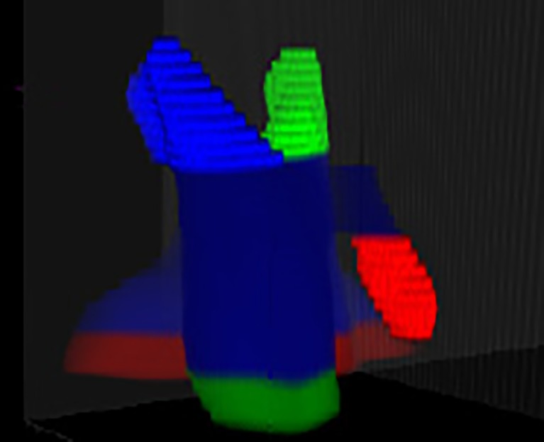
To illustrate the CDOM model, the few samples of FCM segmentation slices (S9, S10 and S11) are considered in Fig. 9. An object in S9 has been divided into three separate objects in S10 and S11, and the centre of the object is as well changed. Euclidean distance of the object centre in S9 has been measured with the centre of the object in S10. The value is greater than the threshold; therefore, the objects in S10 are not connected to the object in S9. In the next slice of the displacement of the objects, the centre is less than the threshold value and each object merges with the corresponding object. The result of dissociation model is depicted in Fig. 10 which shows the six sub-VOIs created by CDOM.
Fig. 9.
A view of the CDOM model procedure
Fig. 10.
Six sub-VOIs created by CDOM
According to the characteristics of angiogenesis, 3D GLCM texture features and 3D compactness features are extracted from dissociated objects by CDOM. ADASYN is used to over-sampling of the minority class in order to obtain an approximately equivalent representation of both classes. The different combinations of features which are listed in Table 2 are used as input for the classifier. Multilayer perceptron (MLP) is a feed forward neural network model which is widely used in analysing the object characteristics in order to recognise the patterns. Matlab neural network toolbox is an interactive environment that provides a suitable context for the implementation of a neural network for clustering, fitting, pattern recognition and time series.
The first step to learning a supervised classifier is to prepare the training data. The CDOM model is used to dissociate the VOIs into sub-VOIs. The sub-VOIs are labelled according to the reporting of two expert radiologists. The 3D GLCM texture features include energy, entropy, correlation, contrast, variance, sum mean, inertia, cluster shade, cluster tendency, homogeneity, max probability, inverse variance and 3D compactness shape features which are extracted from dissociated sub-VOIs with CDOM model.
In this research, the focus is on the binary classification for breast cancer detection on CTLM dataset. The CTLM dataset is obtained from 180 patients, in which a total of 132 instances are labelled normal and the remaining 48 are labelled as abnormal, based on two expert radiologists report and correlation with their mammography and ultrasound images. The proposed dissociation model divides the segmented VOIs into sub-VOIs (5–10 objects for each image). The distribution of negative and positive instances in CTLM dataset is shown in Table 3. According to this figures, the number of negative instances is much higher than the positive instances, which reflect the imbalanced class distribution. To overcome the difficulty of learning associated with the imbalanced dataset, adaptive synthetic sampling (ADASYN) technique [42] is used to create a balanced training data. MLP neural network pattern recognition has been applied to diagnose an abnormality in CTLM images. In order to select the best combination of features on the proposed dissociation model (CDOM) for classification, each group of features are individually trained and assessed by provided classifier.
Table 3.
The number of negative and positive instances in CTLM dataset
| Total | Normal | Abnormal | |
|---|---|---|---|
| Number of patients | 180 | 132 | 48 |
| Number of dissociated object | 1994 | 1939 | 55 |
| Number of dissociated object after apply ADASYN | 3867 | 1939 | 1928 |
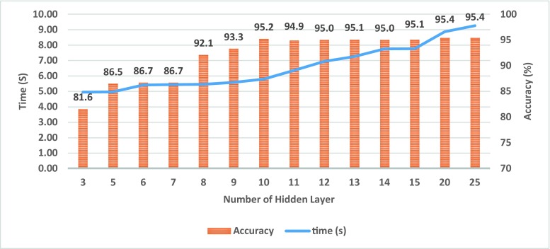
The number of negative and positive instances in CTLM dataset MLPNN method is designed to classify normal and abnormal objects in CTLM image for the diagnosis of breast cancer (Table 3). To obtain the appropriate number of the layer for the proposed MLPNN, Fig. 11 shows the achieved classification accuracy and required time for learning MLPNN by a combination of GLCM 3D and compactness feature (F15) by a different number of hidden layers. Increasing the number of layers does not provide any significant effect on the performance of MLPNN but has led to the increase of learning time. Therefore, based on the results of further experiments, a number of 10 layers have been considered for hidden layers.
Fig. 11.
Accuracy and required time to learn proposed MLPNN method by different number of hidden layer for all combination of GLCM 3D and compactness feature (F15)
The balanced data with ADASYN oversampling are used to train the neural network. Seventy per cent of the input data are used for training, 15% for testing and the rest of the data (15%) for validation. These features are separately transmitted to the network as input data for building models, testing and validation. The training function “trainlm” is used to update weight and bias values based on Levenberg-Marquardt (LM) backpropagation [44, 45]. The trainlm function is often the fastest backpropagation algorithm for a neural network which is frequently advised for supervised learning.
The performance of the proposed MLPNN classifier with the different combination of features is depicted in Fig. 12. The group feature F16 is extracted with sequential forward selection technique and contains 18 features, while F15 included all Harlick’s features and compactness. The overall results show that the combination of each Harlick’s features with compactness features is not sufficient individually to describe characteristics of objects (sub-VOIs). The results show the group feature F15 which contains all Harlick’s features, and compactness has achieved the highest accuracy, sensitivity and specificity. The highest accuracy, sensitivity and specificity are 95.2, 92.4 and 98.1%, respectively. The high number of features used in learning procedure in some systems increases the computation time. Compared to enhance the efficiency of the system by using the high number of features, increasing the learning time is not important in CAD systems, and therefore, all extracted features from dissociated VOIs with CDOM model present higher accuracy, sensitivity and specificity in the proposed CTLM-CAD system.
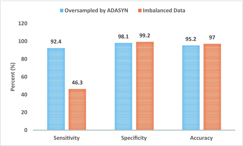
Figure 13 is presented to compare the classifier results with and without ADASYN on the group feature F15 which contains all Harlick’s features and compactness. In the imbalanced dataset, when the number of positive instances is much smaller than the number of negative instances, the sensitivity is low and the specificity is high, as well as high overall accuracy [53].
Fig. 13.
Performance of the proposed MLPNN classifier with and without ADASYN oversampling
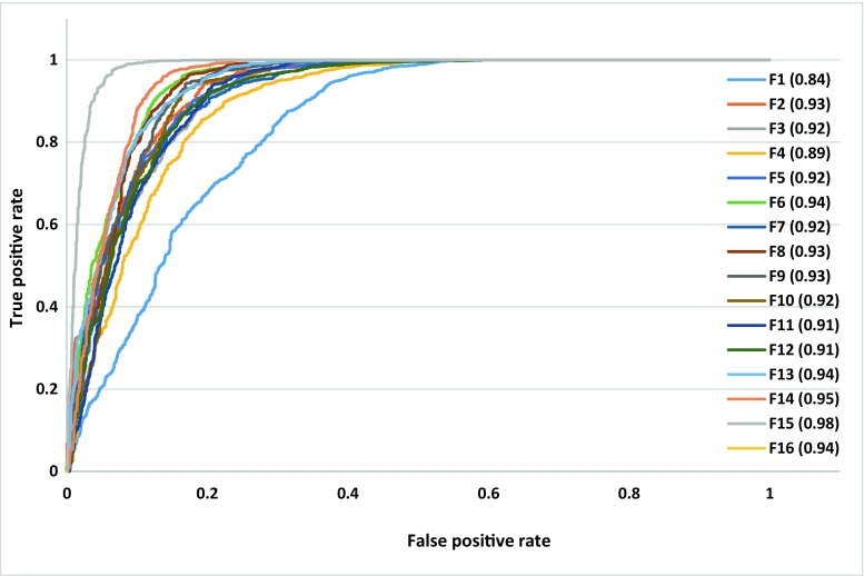
Figure 14 illustrates the ROC and AUROC of proposed classifier using all combination of features (shown in Table 2).The group feature F1 includes three compactness features which achieve the lowest value of AUROC, 0.84. The group features F2–F13 are combination of three compactness features and each Harlick’s feature which introduced in Table 2. The obtained values of AUROC with group features F2–F13 are between 0.89 and 0.94. The group feature F14 contains all 3D GLCM (Harlick’s) features which have obtained the AUROC value equal 0.95. The group feature F15 consists of three compactness features and all 3D GLCM (Harlick’s) features which achieve the highest value of AUROC, 0.98. These results demonstrate usage of a high number of features to learn MLPNN increases CTLM-CAD system performance to diagnose breast cancer.
Fig. 14.
Performance evaluation of the proposed MLPNN classifier with ROC and AUROC values for all combinations of features
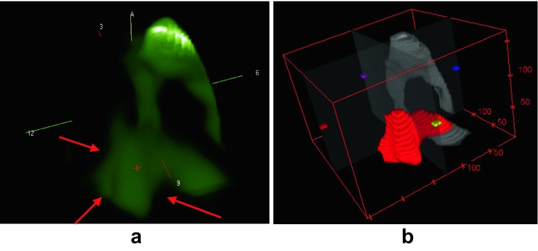
To investigate the proposed CTLM-CAD system in the detection of breast cancer, an automatic diagnosis example has been depicted in Fig. 15. The rendered image by CTLM standalone in front to back projection (FTB) mode is shown in Fig. 15a. The radiologists detect a polypoid-shaped angiogenesis in the posterior segment at 9–10 o’clock which is shown by red arrows in Fig. 15a. The suspicious area in CTLM image has correlated with ultrasound and mammography patient’s images. The red object (Fig. 15b) was detected as a suspicious lesion by proposed CTLM-CAD system and confirmed as an angiogenesis by two expert radiologists. The red object was detected as an abnormal and located in the posterior segment of the breast at 9–10 o’clock (small yellow cube shows 9 o’clock). The shape of angiogenesis detected by the proposed CAD system is similar to polypoid shape.
Fig. 15.
Diagnosis angiogenesis in CTLM images by proposed classifiers. a Rendered CTLM standalone in FTB mode and b MLPNN
Conclusion
In this research, a novel computer-assisted diagnostic (CAD) framework was developed for detecting breast cancer in computed tomography laser mammography (CTLM) images. This CAD system consists of three main components, namely (1) segmentation volume of interests (VOIs), (2) development of dissociation model to disjoint VOIs into sub-VOIs as pre-step of feature extraction, and (3) detection and classification of the abnormality. This research encountered a binary classification for breast cancer detection on CTLM dataset. The CTLM dataset was obtained from 180 patients, in which a total of 132 instances were labelled normal and the remaining 48 were labelled abnormal based on two expert radiologists reporting and correlation with their mammography and ultrasound images. The number of negative instances is too much higher than the positive instances which reflect the imbalanced class distribution.
To overcome the difficulty of learning associated with the imbalanced dataset, adaptive synthetic sampling (ADASYN) technique [42] was applied on dissociated objects. MLP neural network was applied to diagnosis abnormality in CTLM images. The performance evaluation of the proposed classifier in this study was measured with different metrics including accuracy, sensitivity and specificity, ROC curve and AUROC value. The results show that the highest accuracy has been achieved by group feature F15 which is a combination of compactness and all 3D GLCM, which is 95.2%, as well as the highest sensitivity and specificity obtained by MLPNN which are 92.4 and 98.1%, respectively. The highest area under the curve (AUROC) was achieved with group feature F15 which is 0.98.
The most significant limitation of this study was the lack of all forms of angiogenesis in CTLM dataset. Another limitation of this study was the access to Digital Imaging and Communications in Medicine (DICOM) format of CTLM image, which was not provided by the data collection centres. To address this matter, the coronal slices of CTLM images were saved as Tagged Image File Format (TIFF) and used in all procedures.
To achieve the clinical use of the proposed framework, the level of performance and impact of the system in breast cancer detection have to be investigated through a rigorous clinical trial. The CTLM-CAD system has to be tested in multi-centre, multi-reader and multi-cases with and without CAD system.
Various possibilities can be recommended for future work to develop this work such as extract other shape features such as asymmetry to evaluate the effectiveness in classifier performance. Collecting more cancerous CTLM images that include other shapes of angiogenesis such as ringed-shaped and polypoid-shaped to be enhanced the performance of CTLM-CAD system.
Acknowledgements
We gratefully acknowledge who helped us to do our study. Without their continued efforts and support, we would not have been able to gather the dataset and the successful complementation of our work. We also thank Laszlo Meszaros for sharing the dataset, Dr. Ahmad Kamal Bin Md Alif for helping us to review and report CTLM images, and Nur Iylia Roslan for assisting us in the data collection.
Compliance with ethical standards
Funding
This work was funded by the Ministry of Science, Technology & Innovation (MOSTI) Malaysia (Research Grant No. 5457080).
Contributor Information
Afsaneh Jalalian, Phone: +989127811156, Email: jalalian.afsaneh@gmail.com.
Syamsiah Mashohor, Email: syamsiah@upm.edu.my.
Rozi Mahmud, Email: Rozi@upm.edu.my.
Babak Karasfi, Email: Karasfi@qiau.ac.ir.
M. Iqbal Saripan, Email: iqbal@upm.edu.my
Abdul Rahman Ramli, Email: arr@upm.edu.my.
References
- 1.Eid MEE, Hegab HMH, Schindler AE. Role of CTLM in early detection of vascular breast lesions. Egyp J Radiol Nucl Med. 2006;37(1):633–643. [Google Scholar]
- 2.Helbich TH, et al. Mammography screening and follow-up of breast cancer. HAMDAN MEDICAL JOURNAL. 2012;5(1):5–18. doi: 10.7707/hmj.v5i1.104. [DOI] [Google Scholar]
- 3.Carney PA, et al. Individual and combined effects of age, breast density, and hormone replacement therapy use on the accuracy of screening mammography. Annals of internal medicine. 2003;138(3):168–175. doi: 10.7326/0003-4819-138-3-200302040-00008. [DOI] [PubMed] [Google Scholar]
- 4.Boyd NF, et al. Mammographic density and the risk and detection of breast cancer. New England Journal of Medicine. 2007;356(3):227–236. doi: 10.1056/NEJMoa062790. [DOI] [PubMed] [Google Scholar]
- 5.Flöry, D., et al., Advances in breast imaging: a dilemma or progress? Minimally Invasive Breast Biopsies, p. 159–181, 2010.
- 6.Poellinger A, et al. Near-infrared laser computed tomography of the breast. Academic radiology. 2008;15(12):1545. doi: 10.1016/j.acra.2008.07.023. [DOI] [PubMed] [Google Scholar]
- 7.Zhu Q, et al. Benign versus malignant breast masses: optical differentiation with US-guided optical imaging reconstruction 1. Radiology. 2005;237(1):57–66. doi: 10.1148/radiol.2371041236. [DOI] [PMC free article] [PubMed] [Google Scholar]
- 8.Qi J, Ye Z. CTLM as an adjunct to mammography in the diagnosis of patients with dense breast. Clinical imaging. 2013;37(2):289–294. doi: 10.1016/j.clinimag.2012.05.003. [DOI] [PubMed] [Google Scholar]
- 9.Taplin SH, et al. Screening mammography: clinical image quality and the risk of interval breast cancer. American Journal of Roentgenology. 2002;178(4):797–803. doi: 10.2214/ajr.178.4.1780797. [DOI] [PubMed] [Google Scholar]
- 10.Harefa J, Alexander A, Pratiwi M. Comparison classifier: support vector machine (SVM) and K-nearest neighbor (K-NN) in digital mammogram images. Jurnal Informatika dan Sistem Informasi. 2016;2(2):35–40. [Google Scholar]
- 11.Grable, R.J., et al. Optical computed tomography for imaging the breast: first look. in Photonics Taiwan. 2000. International Society for Optics and Photonics.
- 12.Herranz, M. and A. Ruibal, Optical Imaging in Breast Cancer Diagnosis: The Next Evolution. Journal of oncology, p. 1–10, 2012. [DOI] [PMC free article] [PubMed]
- 13.(IDSI), I.D.S. An Innovative Breast Imaging System to Aid in the Detection of Breast Abnormalities. 2016; Available from: http://imds.com/about-computed-tomography-laser-mammography/benefits-of-ctlm.
- 14.Bílková A, Janík V, Svoboda B. Computed tomography laser mammography. Casopis lekaru ceskych. 2009;149(2):61–65. [PubMed] [Google Scholar]
- 15.van de Ven S, et al. Optical imaging of the breast. Cancer Imaging. 2008;8(1):206. doi: 10.1102/1470-7330.2008.0032. [DOI] [PMC free article] [PubMed] [Google Scholar]
- 16.Star, W.M., Diffusion theory of light transport. Optical-thermal response of laser-irradiated tissue, p. 145–201, 2011.
- 17.Floery D, et al. Characterization of benign and malignant breast lesions with computed tomography laser mammography (CTLM): initial experience. Investigative radiology. 2005;40(6):328–335. doi: 10.1097/01.rli.0000164487.60548.28. [DOI] [PubMed] [Google Scholar]
- 18.Orchard MT, Bouman CA. Color quantization of images. Signal Processing, IEEE Transactions on. 1991;39(12):2677–2690. doi: 10.1109/78.107417. [DOI] [Google Scholar]
- 19.A.Jalalian, S. M., R. Mahmud, B. Karasfi, M. I. Saripan, A. R. Ramli, N. Bahri, S. A/P Suppiah, Computed Automatic 3D Segmentation Methods in Computed Tomography Laser Mammography, in Advances in Computing, Electronics and Communication - ACEC. 2015. p. 204–208, 2015.
- 20.Jalalian, A., et al. 3D reconstruction for volume of interest in computed tomography laser mammography images. in 2015 I.E. Student Symposium in Biomedical Engineering & Sciences (ISSBES). IEEE,p.16–20, 2015.
- 21.Cheng, I., et al. Ground truth delineation for medical image segmentation based on Local Consistency and Distribution Map analysis. in Engineering in Medicine and Biology Society (EMBC), 2015 37th Annual International Conference of the IEEE. 2015. IEEE. [DOI] [PubMed]
- 22.Jaccard P. The distribution of the flora in the alpine zone. New phytologist. 1912;11(2):37–50. doi: 10.1111/j.1469-8137.1912.tb05611.x. [DOI] [Google Scholar]
- 23.Dice LR. Measures of the amount of ecologic association between species. Ecology. 1945;26(3):297–302. doi: 10.2307/1932409. [DOI] [Google Scholar]
- 24.Kohlberger, T., et al., Evaluating segmentation error without ground truth, in Medical Image Computing and Computer-Assisted Intervention–MICCAI 2012., Springer. p. 528–536, 2012. [DOI] [PubMed]
- 25.Jalalian A, et al. Computer-aided detection/diagnosis of breast cancer in mammography and ultrasound: a review. Clinical imaging. 2013;37(3):420–426. doi: 10.1016/j.clinimag.2012.09.024. [DOI] [PubMed] [Google Scholar]
- 26.Kurani, A.S., et al. Co-occurrence matrices for volumetric data. in 7th IASTED International Conference on Computer Graphics and Imaging, Kauai, USA. 2004.
- 27.Lee H, Chen Y-PP. Image based computer aided diagnosis system for cancer detection. Expert Systems with Applications. 2015;42(12):5356–5365. doi: 10.1016/j.eswa.2015.02.005. [DOI] [Google Scholar]
- 28.Haralick, R.M., K. Shanmugam, and I.H. Dinstein, Textural features for image classification. Systems, Man and Cybernetics, IEEE Transactions on, (6): p. 610–621, 1973.
- 29.Gao, X., et al., Texture-based 3D image retrieval for medical applications. Proceedings of IADIS e-Health. Freiburg, Germany, 2010.
- 30.Albregtsen, F., Statistical texture measures computed from gray level coocurrence matrices. Image processing laboratory, department of informatics, university of oslo,: p. 1–14, 2008.
- 31.Hanusiak R, et al. Writer verification using texture-based features. International Journal on Document Analysis and Recognition (IJDAR) 2012;15(3):213–226. doi: 10.1007/s10032-011-0166-4. [DOI] [Google Scholar]
- 32.Mostaço-Guidolin, L.B., et al., Collagen morphology and texture analysis: from statistics to classification. Scientific reports, 3, 2013. [DOI] [PMC free article] [PubMed]
- 33.Yang X, et al. Ultrasound GLCM texture analysis of radiation-induced parotid-gland injury in head-and-neck cancer radiotherapy: an in vivo study of late toxicity. Medical physics. 2012;39(9):5732–5739. doi: 10.1118/1.4747526. [DOI] [PMC free article] [PubMed] [Google Scholar]
- 34.Žunić J, Hirota K, Rosin PL. A Hu moment invariant as a shape circularity measure. Pattern Recognition. 2010;43(1):47–57. doi: 10.1016/j.patcog.2009.06.017. [DOI] [Google Scholar]
- 35.Žunić, J., K. Hirota, and C. Martinez-Ortiz. Compactness measure for 3d shapes. in Informatics, Electronics & Vision (ICIEV), 2012 International Conference on. 2012. IEEE.
- 36.Bribiesca E. An easy measure of compactness for 2D and 3D shapes. Pattern Recognition. 2008;41(2):543–554. doi: 10.1016/j.patcog.2007.06.029. [DOI] [Google Scholar]
- 37.Bribiesca E. A measure of compactness for 3D shapes. Computers & Mathematics with Applications. 2000;40(10):1275–1284. doi: 10.1016/S0898-1221(00)00238-8. [DOI] [Google Scholar]
- 38.Xu D, Li H. Geometric moment invariants. Pattern Recognition. 2008;41(1):240–249. doi: 10.1016/j.patcog.2007.05.001. [DOI] [Google Scholar]
- 39.Saeys Y, Inza I, Larrañaga P. A review of feature selection techniques in bioinformatics. bioinformatics. 2007;23(19):2507–2517. doi: 10.1093/bioinformatics/btm344. [DOI] [PubMed] [Google Scholar]
- 40.David, S.K. and M.K. Siddiqui, Perspective of Feature Selection Techniques in Bioinformatics. 2011.
- 41.Rahman MM, Davis D. Addressing the class imbalance problem in medical datasets. International Journal of Machine Learning and Computing. 2013;3(2):224–228. doi: 10.7763/IJMLC.2013.V3.307. [DOI] [Google Scholar]
- 42.He, H., et al. ADASYN: Adaptive synthetic sampling approach for imbalanced learning. in Neural Networks, 2008. IJCNN 2008.(IEEE World Congress on Computational Intelligence). IEEE International Joint Conference on. 2008. IEEE.
- 43.Guan, S., et al. Deep Learning with MCA-based Instance Selection and Bootstrapping for Imbalanced Data Classification. in The First IEEE International Conference on Collaboration and Internet Computing (CIC). 2015.
- 44.Marquardt DW. An algorithm for least-squares estimation of nonlinear parameters. Journal of the society for Industrial and Applied Mathematics. 1963;11(2):431–441. doi: 10.1137/0111030. [DOI] [Google Scholar]
- 45.Vacic, V., Summary of the training functions in Matlab’s NN toolbox. Computer Science Department at the University of California, 2005.
- 46.Castellino RA. Computer aided detection (CAD): an overview. Cancer Imaging. 2005;5(1):17–19. doi: 10.1102/1470-7330.2005.0018. [DOI] [PMC free article] [PubMed] [Google Scholar]
- 47.James D, Clymer BD, Schmalbrock P. Texture detection of simulated microcalcification susceptibility effects in magnetic resonance imaging of breasts. Journal of Magnetic Resonance Imaging. 2001;13(6):876–881. doi: 10.1002/jmri.1125. [DOI] [PubMed] [Google Scholar]
- 48.Fawcett T. An introduction to ROC analysis. Pattern recognition letters. 2006;27(8):861–874. doi: 10.1016/j.patrec.2005.10.010. [DOI] [Google Scholar]
- 49.Sonego P, Kocsor A, Pongor S. ROC analysis: applications to the classification of biological sequences and 3D structures. Briefings in bioinformatics. 2008;9(3):198–209. doi: 10.1093/bib/bbm064. [DOI] [PubMed] [Google Scholar]
- 50.Fawcett, T., ROC graphs: Notes and practical considerations for researchers. 2004.
- 51.Bradley AP. The use of the area under the ROC curve in the evaluation of machine learning algorithms. Pattern Recognition. 1997;30(7):1145–1159. doi: 10.1016/S0031-3203(96)00142-2. [DOI] [Google Scholar]
- 52.Hanley JA, McNeil BJ. The meaning and use of the area under a receiver operating characteristic (ROC) curve. Radiology. 1982;143(1):29–36. doi: 10.1148/radiology.143.1.7063747. [DOI] [PubMed] [Google Scholar]
- 53.Lin, W.-J. and J.J. Chen, Class-imbalanced classifiers for high-dimensional data. Briefings in bioinformatics, p. bbs006, 2012. [DOI] [PubMed]


