A 3D Model-Based Simulation of Demyelination to Understand its Effects on Diffusion Tensor Imaging

Abstract

Demyelination is the progressive damage to the myelin sheath, a protective covering that surrounds a nerve’s axon. Due to its high sensitivity to microscopic tissue changes, diffusion tensor imaging (DTI) is a powerful means of detecting signs of demyelination and axonal injury. In this paper, we present a 3D virtual model capable of simulating the complex Brownian motion of water molecules in a bundle of myelinated axons and glial cells for the purpose of synthesizing DTI data, characterizing and verifying the impact of demyelination on DTI. Our model consists of a highly detailed and realistic 3D representation of biological fiber bundles, with a myelin sheath covering the axons and glial cells in between them. The system simulates the Brownian motion of molecules to extract diffusion data. We perform our experiment for progressive stages of demyelination and demonstrate its effect on DTI measurements.

I. Introduction

Myelin insulation around the axons plays an important role in cognitive performance as it maintains the conductivity and reliability of neural transmission. Multiple sclerosis (MS), an autoimmune disease damaging the central nervous system is the most common cause of demyelination and affects 2.3 million people worldwide [1]. Myelin damage can also be caused by viral infections and chemotherapy induced neurotoxicity [2]. DTI is an exceptional tool for non-invasive studies of neurological diseases that cause extensive damage to neural pathways in the central nervous system [3]. The key principle behind DTI is that the natural Brownian motion of water molecules in the brain is not free (isotropic), but is constrained (anisotropic) by cell membranes, myelin sheaths, and macromolecules. Therefore, characterizing the diffusion patterns reveals important details about the microstructure and directionality of the fibers themselves.

In recent years DTI, a diffusion weighted magnetic resonance imaging (MRI) technique, is increasingly used as a biomarker to diagnose demyelination [4, 5]. Unlike conventional MRI, which is not sensitive to diffusion, magnetic field gradients are applied from different spatial directions to obtain a diffusion-weighted signal and estimate the diffusion along those directions. DTI does not directly reveal the structure and connectivity of nerve fibers. This information is inferred from the diffusion tensor computed as an indirect measurement of the degree of anisotropy and axon orientation inside a voxel [6]. DTI properties obtained from a single voxel are therefore statistical parameters that result from the integration of the combined diffusions that occur at a microscopic scale. This implies an inherent limitation as DTI assumes some homogeneity inside a millimetric voxel and cannot completely describe the complex axonal architecture on a microscopic scale. Furthermore, the observed diffusion is a joint result of water pools located in different tissue compartments (e.g., intra-cellular, extra-cellular, or myelin water) [7, 8]. Changes in anisotropy often cannot be traced to specific water sources within the neural structure, and it is still unclear if these changes are due to a loss of myelin, a decrease of axonal density or other underlying mechanisms. Investigating tissue specific information requires acquisition and processing methods that differ from conventional DTI techniques [8]. This highlights the need to provide ground truth in order to differentiate and categorize the different types of tissue damage and understand how they affect DTI measurements.

In this work, we propose a 3D virtual model of myelinated neural fibers to simulate the diffusion of water molecules and generate synthetic DTI data. Several methods have successfully modeled fiber bundles to acquire synthetic data and validate diffusion-weighted imaging techniques [9, 10, 11], but no attempts have taken into account the presence of myelin due to the difficulty of representing tightly packed axons in extremely narrow spaces. For a more accurate representation, we also take into account glial cells that make up a significant volume of the extra-axonal space with an axon to glia ratio of 1:3.76 in the cerebral cortex [12, 13]. This undoubtedly affects the diffusion of molecules as well. The novelty of our work is that it brings to bear a state of the art 3D modeling methodology that can produce highly detailed and flexible models of myelinated axons and glial cells to simulate a progressive demyelination and study its impact on DTI.

II. Building the 3D Model

Our approach relies on Blender: a powerful 3D modeling software used for computer graphics animation, visual effects rendering, 3D print modeling, as well as video games applications. Blender’s physics engine can simulate complex physical scenes with several interacting objects and forces. A scripting option also allows users to programmatically generate objects, forces and simulate events. Our system is implemented within Blender using custom Python scripts.

A. Generating Axons and Glial Cells

Blender can create virtual spaces containing 3D objects in any desired shape and size. We wish to generate a voxel containing a bundle of myelinated axons and glia, and simulate the diffusion of water molecules within the voxel such that cell membranes act as barriers. In this study we will only focus on modeling fibers located in the corpus callosum where all the axons are parallel (Fig. 1-A). Our design relies on highly accurate descriptions of the biological geometry [13, 14, 15].

Figure 1.

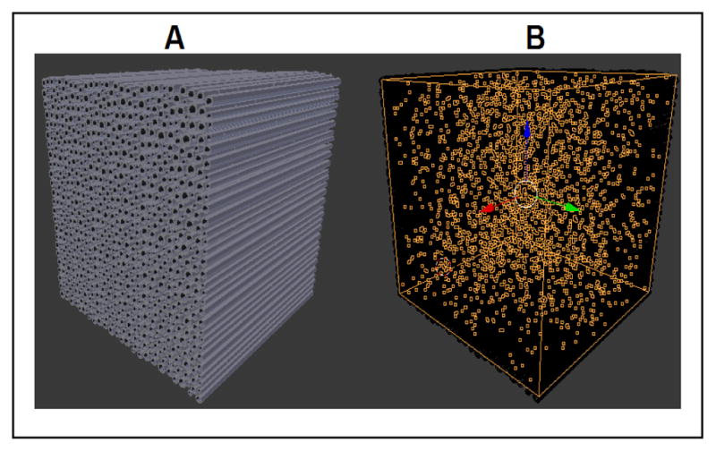
Blender rendering of our model with parallel axons (A) and the diffusing particles (B).

Axon sizes vary greatly from 0.1 μm up to 12 μm depending on the region of the brain. The largest axons can be found in the corpus callosum while the smallest are found at the periphery. In turn, the thickness of a fully developed myelin sheath varies with respect to the radius of its corresponding axon in a non-linear fashion [15]. The myelin thickness represents around 50% of the total diameter for the smallest axons (<2.5 μm), it drops to 30–40% in the mid-range (2.5–6 μm), and it represents less than 10% of the diameter for large axons (>6 μm). Glial cells are broadly classified as macroglia and microglia. For our purposes we only model macroglia of which astrocytes and oligodendrocytes are the most abundant comprising over 90% of all glia in the central nervous system [13]. These cells are star-shaped because of their numerous processes radiating in all directions that can extend up to 50 μm. Our glia design entails diamond and star-shaped faces with a width of 2.5 μm, representing the main cell body, placed between the axons and randomly distributed in the simulation space with an axon to glia ratio of 1:3.5.

B. Simulating Myelin Degeneration

The model can simulate a gradual myelin decay. The rate of demyelination is the same for all axons regardless of size and is arranged as a percentage reduction of the original myelin width. Fig. 2 demonstrates a demyelination effect on a collection of parallel axons in the corpus callosum where the thickness is reduced to 80% its original width (Fig. 2-A), followed by a more severe reduction to 20% (Fig. 2-B). A noticeable consequence is the expansion of the extra-axonal space which will inadvertently alter the diffusion process and DTI measurements [16].

Figure 2.

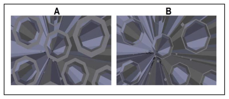
Axons with enveloping myelin at 80% original thickness (A) and 20% original thickness (B).

III. Simulating the Diffusion

A key feature in Blender is its particle system. It is primarily applied to simulate phenomena such as fire, dust, clouds, smoke, or liquid particles. To stay true to Blender’s terminology, water molecules will be referred to as particles. Particles are generated uniformly across the voxel (Fig. 1-B) and are located either in the extra-axonal space (between axons) or intra-axonal space (inside individual axons). A Brownian force causes them to move and interact with the surrounding axons and glia tissue, making the diffusion bounded. The diffusion coefficient D₀ of water molecules ranges from 1 to 3 mm²/s at body temperature (37°C) [17]. However, Blender parameters that control the rate of particle diffusion are dimensionless scalars and need to be properly calibrated in order achieve a desired diffusion rate.

For this purpose, we devise a free diffusion calibration test where particles move in an isotropic environment with no obstacles or boundaries. We generate N particles at a single point of origin and diffuse them over a period Δt. We obtain each particle’s displacement vector x_i representing the total distance traveled by each particle i. We define < x² > as the expectation value of the squared displacement vectors x_i [18] and calculate it for N particles as

$$<x^2>=\frac{{\mathrm{\sum }}_{i=1}^{\mathrm{N}}{x}_i^2}{\mathrm{N}}.$$ (1)

The expectation value < x² > is also scaled to the diffusion coefficient D₀ and is calculated from the Einstein equation [18]

$$\sqrt{<x^2>}=\sqrt{6D_0\mathrm{\Delta }t}.$$ (2)

Using these definitions, we can determine from (2) the expectation value for a desired diffusion coefficient D₀ and subsequently calibrate Blender’s parameters such that the output < x² > calculated from (1) approximates our target value. For example, to obtain a diffusion rate of D₀ = 2.6 mm²/s over 100 ms, (2) yields an expectation value of < x² > = 1560. We then calibrate Blender’s diffusion parameters in our test simulation so that < x² > from (1) approaches the same value. This is illustrated in Fig. 3 where our system is calibrated to closely approximate a diffusion rate of 2.6 mm²/s.

Figure 3.

(A) $\sqrt{<x^2>}$ calculated from (2) for D₀ raging from 1 to 3 mm²/s. (B) Experimental $\sqrt{<x^2>}$ obtained from (1).

IV. Extracting DTI Properties

The simplest and most common approach to acquire diffusion weighted MRI is with a pulsed-gradient spin echo (PGSE) sequence. Fig. 4 describes a typical PGSE sequence containing two periods of equal duration T for a total echo time TE = 2T [19]. At t = 0, a 90° RF pulse magnetizes the hydrogen protons (spins), followed by a gradient pulse at an arbitrary time t₁ with strength g and duration δ that dephases the magnetization of the spins. In the next period, a 180° RF pulse refocuses the spins, and a second gradient pulse of equal strength and duration but opposite direction rephases the magnetization of the spins. The second gradient is separated from the first by a duration Δ.

Figure 4.

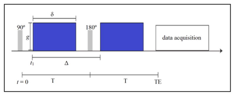
Pulsed-gradient spin echo (PGSE) sequence with pulse strength g, width δ, and distance Δ between the two pulses.

For non-diffusing particles, the phases induced by both gradient pulses will cancel out, resulting in no change in the nuclear magnetic resonance (NMR) signal. However, when a particle moves, there will be a phase difference resulting in an attenuation of the NMR signal proportional to the distance travelled in the direction of the gradient. The signal attenuation is described by

$$S=S_0{\mathrm{e}}^{-bD},$$ (3)

where S is the diffusion weighted signal, S₀ is the signal without any diffusion weighted gradients, D is the apparent diffusion coefficient (ADC), and b (called b-value) is the amount of diffusion-weighting given by the properties of the gradient pulse g, δ, Δ, and the gyromagnetic ratio γ defined as

$$b={\mathrm{\gamma }}^2{g}^2{\mathrm{\delta }}^2(\mathrm{\Delta }-\frac{\mathrm{\delta }}{3}).$$ (4)

The ADC is a measure of diffusion in the direction of the applied gradient. Using it instead of the diffusion coefficient D₀ indicates that the diffusion is hindered. In the absence of diffusion sensitizing gradients (i.e., g = 0) the measured MRI signal S equals S₀. When gradients are applied (i.e., g ≠ 0) the measured signal S is attenuated and we calculate the ADC by solving for D in (3).

Blender does not emit RF pulses to magnetize the particles, and the diffusing particles in turn do not re-emit NMR signals, therefore we cannot directly measure the signal attenuation S and find the ADC. Our simulation works by diffusing particles to generating a list of displacement vectors z_i for each particles i inside the simulation space. Since the signal attenuation depends on the phase shift of diffusing particles, we can find S from the accumulated phase φ_i(TE) of each particle i over a period TE [19] calculated as

$${\mathrm{\phi }}_i(\text{TE})=\mathrm{\gamma }g\left\{{\int }_{t_1}^{t_1+\mathrm{\delta }}{z}_i(t)\mathrm{d}t+{\int }_{t_1+\mathrm{\Delta }}^{t_1+\mathrm{\Delta }+\mathrm{\delta }}{z}_i(t)\mathrm{d}t\right\}.$$ (5)

Here z_i is the displacement only along the direction of the gradient (i.e., the z-direction). Fig. 4 shows how the first integral relates to the phase accumulated during the first gradient pulse, while the second integral relates to the phase accumulated during the second gradient pulse. The normalized attenuation of the echo signal [19] is given as

$$S=S_0{\int }_{-\infty }^{\infty }\mathrm{P}(\mathrm{\phi },\text{TE})cos\mathrm{\phi }\mathrm{d}\mathrm{\phi },$$ (6)

where P(φ,TE) is the phase-distribution function. By definition it must be a normalized function such that ${\int }_{-\infty }^{\infty }\mathrm{P}(\mathrm{\phi },\text{TE})\mathrm{d}\mathrm{\phi }=1$. The integral in (6) is the expected value of the cosine of the phases, and assuming the distribution to be Gaussian, we can rewrite it as,

$$S=S_0\frac{{\mathrm{\sum }}_{i=1}^{\mathrm{N}}cos{\mathrm{\phi }}_i}{\mathrm{N}},$$ (7)

where N is the number of particles. Finally we can find the ADC by combining the right hand sides of (3) and (7), and solve for D in

$${\mathrm{e}}^{-bD}=\frac{{\mathrm{\sum }}_{i=1}^{\mathrm{N}}cos{\mathrm{\phi }}_i}{\mathrm{N}}.$$ (8)

We repeat this process to obtain the ADC for multiple gradient directions and compute the diffusion tensor and other DTI metrics [20]. We are interested in finding the mean (MD), axial (AD), radial (RD) diffusivities, and the fractional anisotropy (FA). MD, AD and RD represent the magnitudes of diffusivity in different directions. AD is the measure along the main axis of diffusion, RD along non-axial directions and MD is the averaged diffusivity in all directions. FA is a 0 to 1 scalar describing the degree of anisotropy, a value of 0 denotes an isotropic diffusion equal in all directions, while a value of 1 denotes a highly anisotropic diffusion confined to a single direction.

V. Simulation And Results

The system generates a model of myelinated axons and glial cells located in the corpus callosum. The simulation space consists of around 4000 parallel axons and 15000 glia located inside a 100x100x100 μm voxel. Axon diameters with a fully developed myelin sheath range from 2 μm to 10 μm, while glia diameters are fixed at 2.5 μm. For 20 gradient directions, we generate and diffuse 50000 particles at a diffusion rate of D₀ = 2.5 mm²/s for a duration TE = 100 ms (δ = 19 ms, Δ = 56 ms), and b = 1000 mm²/s. From the coordinates of each particle we find the displacement vectors and compute DTI metrics (i.e., MD, AD, RD, FA). To capture the effect of demyelination we repeat this process by incrementally reducing the myelin sheath by 10% of its original width. The results are shown in Fig. 5–6.

Figure 5.

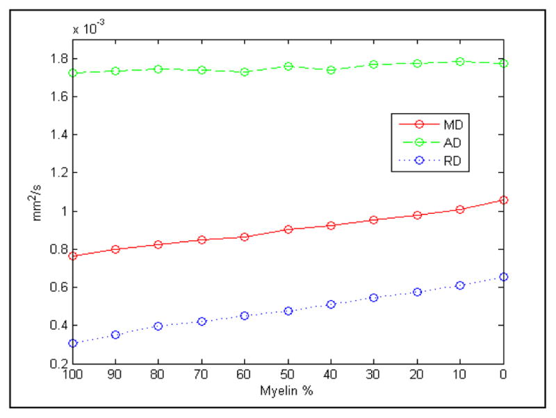
Change in MD, AD and RD due to myelin reduction.

Figure 6.

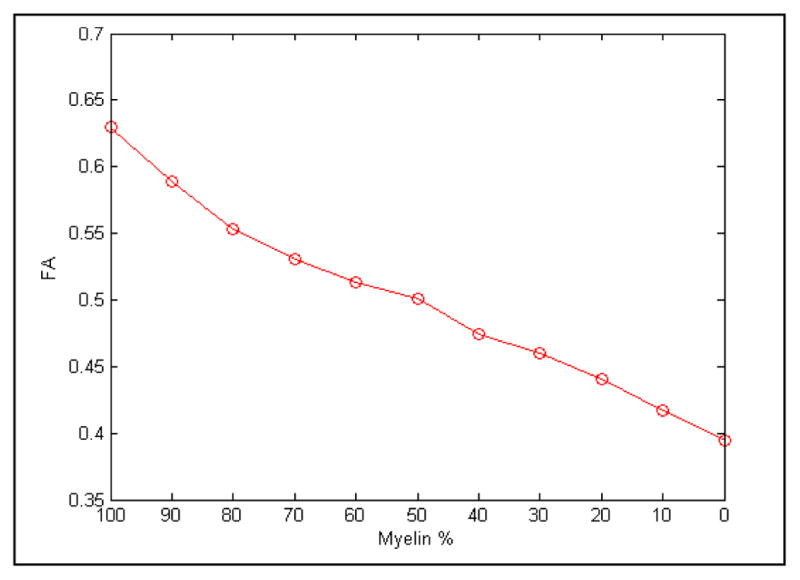
Change in FA due to myelin reduction.

When the myelin is fully developed our recorded AD is much higher than the radial and mean diffusivities (Fig. 5), signifying a diffusion that is mainly confined to a single axial direction. As the width of myelin decreases the extra-axonal space increases giving the particles more free range to diffuse thereby reducing the directionality of movement and making the diffusion more isotropic (or less anisotropic). This effect is highlighted by a decrease in FA from 0.63 to 0.39, and an increase in RD from 0.3x10⁻³ mm²/s to 0.66x10⁻³ mm²/s while the AD remains steady, demonstrating a rise in particle movement in non-axial directions.

We also see a small rise in MD from 0.75x10⁻³ mm²/s to 1.06x10⁻³ mm²/s (Fig. 5). Our simulation doesn’t record any significant variations in AD as it tends to be variable in white matter changes and pathology.

VI. Conclusion And Future Works

We demonstrated a novel 3D model of the corpus callosum capable of accurately simulating water particle diffusion in a tightly compacted fiber bundle comprising of myelinated axons and glial cells, and generating synthetic DTI data for the purpose of characterizing the effect of demyelination.

We look to expand on this effort to model other areas of the brain with different fiber configurations such as crossing, kissing, and bending fibers. We also wish to significantly enlarge our model sizes from a micrometer to a millimeter scale to match the size of real MRI voxels and potentially perform studies on tracking over several adjacent voxels. Another known outcome of severe and chronic demyelination is the compaction of axonal neurofilament causing lasting damage on cognitive function. Compaction causes the axons to move closer and fill the extra-axonal space left by the receding myelin. We look to expand our model beyond demyelination to simulate axon compaction and study its effect on DTI measurements as well.

References

- 1.Love S. Demyelinating diseases. J Clin Pathol. 2006 Nov;59:1151–1159. doi: 10.1136/jcp.2005.031195. [DOI] [PMC free article] [PubMed] [Google Scholar]
- 2.Park SB, Goldstein D, Krishnan AV, Lin CSY, Friedlander ML, Cassidy J, Koltzenburg M, Kiernan MC. Chemotherapy-induced peripheral neurotoxicity: A critical analysis. CA: Cancer J Clin. 2013 Nov;63:419–437. doi: 10.3322/caac.21204. [DOI] [PubMed] [Google Scholar]
- 3.Fox RJ, Cronin T, Lin J, Wang X, Sakaie K, Ontaneda D, Mahmoud SY, Lowe MJ, Phillips MD. Measuring myelin repair and axonal loss with diffusion tensor imaging. AJNR Am J Neuroradiol. 2011 Jan;32:85–91. doi: 10.3174/ajnr.A2238. [DOI] [PMC free article] [PubMed] [Google Scholar]
- 4.Aung WY, Mar S, Benzinger TLS. Diffusion tensor MRI as a biomarker in axonal and myelin damage. Imaging Med. 2013 Oct;5:427–440. doi: 10.2217/iim.13.49. [DOI] [PMC free article] [PubMed] [Google Scholar]
- 5.Sbardella E, Tona F, Petsas N, Pantano P. DTI measurement in multiple sclerosis: Evaluation of brain damage and clinical implications. Mult Scler Int. 2013 Mar;2013 doi: 10.1155/2013/671730. [DOI] [PMC free article] [PubMed] [Google Scholar]
- 6.Le Bihan D, Mangin JF, Poupon C, Clark CA, Pappata S, Molko N Chabriat Diffusion H. Tensor imaging: Concepts and applications. J Magn Reson Imaging. 2001 Apr;13:534–546. doi: 10.1002/jmri.1076. [DOI] [PubMed] [Google Scholar]
- 7.Beaulieu C. The basis of anisotropic water diffusion in the nervous system - a technical review. NMR Biomed. 2002 Dec;15:435–455. doi: 10.1002/nbm.782. [DOI] [PubMed] [Google Scholar]
- 8.Avram AV, Guidon A, Song AW. Myelin water weighted diffusion tensor imaging. NeuroImage. 2010 Oct;53:132–138. doi: 10.1016/j.neuroimage.2010.06.019. [DOI] [PubMed] [Google Scholar]
- 9.Yeh C, Schmitt B, Le Bihan D, Li-Schlittgen J, Lin C, Poupon C. Diffusion microscopist simulator: A general monte carlo simulation system for diffusion magnetic resonance imaging. PloS One. 2013 Oct;8 doi: 10.1371/journal.pone.0076626. [DOI] [PMC free article] [PubMed] [Google Scholar]
- 10.Perrone D, Jeurissen B, Aelterman J, Roine T, Sijbers J, Pizurica A, Leemans A, Philips W. D-BRAIN: Anatomically accurate simulated diffusion MRI brain data. PloS One. 2016 Mar;10 doi: 10.1371/journal.pone.0149778. [DOI] [PMC free article] [PubMed] [Google Scholar]
- 11.Neher PF, Laun FB, Stieltjes B, Maier-Hein KH. Fiberfox: Facilitating the creation of realistic white matter software phantoms. Magn Reson Med. 2013 Dec;72:1460–1470. doi: 10.1002/mrm.25045. [DOI] [PubMed] [Google Scholar]
- 12.Azevedo FA, Carvalho LR, Grinberg LT, Farfel JM, Ferretti RE, Leite RE, Filho WJ, Lent R, Herculano-Houzel S. Equal numbers of neuronal and nonneuronal cells make the human brain an isometrically scaled-up primate brain. J Comp Neurol. 2016 Mar;513:532–541. doi: 10.1002/cne.21974. [DOI] [PubMed] [Google Scholar]
- 13.Pelvig DP, Pakkenberg H, Stark AK, Pakkenberg B. Neocortical glial cell numbers in human brains. Neurobiol Aging. 2008 Nov;29 doi: 10.1016/j.neurobiolaging.2007.04.013. [DOI] [PubMed] [Google Scholar]
- 14.Le Bihan D. The ‘wet mind’: water and functional neuroimaging. Phys Med Biol. 2007 Apr;52:57–90. doi: 10.1088/0031-9155/52/7/R02. [DOI] [PubMed] [Google Scholar]
- 15.Fraher J, Dockery P. A strong myelin thickness-axon size correlation emerges in developing nerves despite independent growth of Both Parameters. J Anat. 1998 Aug;193:195–201. doi: 10.1046/j.1469-7580.1998.19320195.x. [DOI] [PMC free article] [PubMed] [Google Scholar]
- 16.Chen KC, Nicholson C. Changes in brain cell shape create residual extracellular space volume and explain tortuosity behavior during osmotic challenge. Proc Natl Acad Sci USA. 2000 Jul;:97. doi: 10.1073/pnas.150338197. [DOI] [PMC free article] [PubMed] [Google Scholar]
- 17.Chenevert TL. Diffusion-weighted MR imaging: applications in the body. Heidelberg: Springer; 2010. Principles of diffusion-weighted imaging (DW-MRI) as applied to the body; pp. 4–17. [Google Scholar]
- 18.Stieltjes B, Brunner RM, Fritzsche KH, Laun FB. Introduction to Diffusion Imaging. Diffusion Tensor Imaging: Introduction and Atlas. ch 1 Springer; 2013. [Google Scholar]
- 19.Price WS. Concepts in Magnetic Resonance. Wiley; 1997. Pulsed-field gradient nuclear magnetic resonance as a tool for studying translational diffusion: Part 1. Basic theory; pp. 299–336. [Google Scholar]
- 20.Jiang H, van Zijl PCM, Kim J, Pearlson GD, Mori S. DtiSudio: Resource program for diffusion tensor computation and fiber bundle tracking. Comput Methods Programs Biomed. 2006 Jan;81:106–116. doi: 10.1016/j.cmpb.2005.08.004. [DOI] [PubMed] [Google Scholar]