Observation- and Model-Based Estimates of Particulate Dry Nitrogen Deposition to the Oceans

Abstract

Anthropogenic nitrogen (N) emissions to the atmosphere have increased significantly the deposition of nitrate (NO₃⁻) and ammonium (NH₄⁺) to the surface waters of the open ocean, with potential impacts on marine productivity and the global carbon cycle. Global-scale understanding of the impacts of N deposition to the oceans is reliant on our ability to produce and validate models of nitrogen emission, atmospheric chemistry, transport and deposition. In this work, ~2900 observations of aerosol NO₃⁻ and NH₄⁺ concentrations, acquired from sampling aboard ships in the period 1995 – 2012, are used to assess the performance of modelled N concentration and deposition fields over the remote ocean. Three ocean regions (the eastern tropical North Atlantic, the northern Indian Ocean and northwest Pacific) were selected, in which the density and distribution of observational data were considered sufficient to provide effective comparison to model products. All of these study regions are affected by transport and deposition of mineral dust, which alters the deposition of N, due to uptake of nitrogen oxides (NO_x) on mineral surfaces.

Assessment of the impacts of atmospheric N deposition on the ocean requires atmospheric chemical transport models to report deposition fluxes, however these fluxes cannot be measured over the ocean. Modelling studies such as the Atmospheric Chemistry and Climate Model Intercomparison Project (ACCMIP), which only report deposition flux are therefore very difficult to validate for dry deposition. Here the available observational data were averaged over a 5° × 5° grid and compared to ACCMIP dry deposition fluxes (ModDep) of oxidised N (NO_y) and reduced N (NH_x) and to the following parameters from the TM4-ECPL (TM4) model: ModDep for NO_y, NH_x and particulate NO₃⁻ and NH₄⁺, and surface-level particulate NO₃⁻ and NH₄⁺ concentrations. As a model ensemble, ACCMIP can be expected to be more robust than TM4, while TM4 gives access to speciated parameters (NO₃⁻ and NH₄⁺) that are more relevant to the observed parameters and which are not available in ACCMIP. Dry deposition fluxes (CalDep) were calculated from the observed concentrations using estimates of dry deposition velocities. Model – observation ratios, weighted by grid-cell area and numbers of observations, (R_A,n) were used to assess the performance of the models. Comparison in the three study regions suggests that TM4 over-estimates NO₃⁻ concentrations (R_A,n = 1.4 – 2.9) and under-estimates NH₄⁺ concentrations (R_A,n = 0.5 – 0.7), with spatial distributions in the tropical Atlantic and northern Indian Ocean not being reproduced by the model. In the case of NH₄⁺ in the Indian Ocean, this discrepancy was probably due to seasonal biases in the sampling. Similar patterns were observed in the various comparisons of CalDep to ModDep (R_A,n = 0.6 – 2.6 for NO₃⁻, 0.6 – 3.1 for NH₄⁺). Values of R_A,n for NH_x CalDep - ModDep comparisons were approximately double the corresponding values for NH₄⁺ CalDep - ModDep comparisons due to the significant fraction of gas-phase NH₃ deposition incorporated in the TM4 and ACCMIP NH_x model products. All of the comparisons suffered due to the scarcity of observational data and the large uncertainty in dry deposition velocities used to derive deposition fluxes from concentrations. These uncertainties have been a major limitation on estimates of the flux of material to the oceans for several decades. Recommendations are made for improvements in N deposition estimation through changes in observations, modelling and model – observation comparison procedures. Validation of modelled dry deposition requires effective comparisons to observable aerosol-phase species concentrations and this cannot be achieved if model products only report dry deposition flux over the ocean.

1 Introduction

Global emissions of inorganic nitrogen (i.e. all nitrogen (N) species, excluding N₂) to the atmosphere have likely increased by factors of 3–4 since the onset of industrialisation in the mid-nineteenth century (Duce et al., 2008; Galloway et al., 2008). Major sources include the emission of nitrogen oxides (NO_x) as a by-product of combustion (Galloway et al., 2004) and ammonia (NH₃) emissions resulting from fertilizer application and intensive livestock-rearing practices (Bouwman et al., 1997). On-going implementation of emission controls (mostly affecting NO_x) and global economic development will lead to further changes in both the magnitude and spatial distribution of nitrogen emissions over the coming decades (e.g. Dentener et al., 2006; Lamarque et al., 2013a).

Nitrogen deposition impacts both terrestrial and marine ecosystems. N is a limiting nutrient for primary producers over ~70% of the global ocean (Duce et al., 2008). Its deposition enhances primary productivity in low-nitrogen marine ecosystems (e.g. Zamora et al., 2010; Singh et al., 2012) and potentially drives ecological shifts through changes in nutrient regimes (Kim et al., 2011; Chung et al., 2011; Shi et al., 2012; Mourino-Carballido et al., 2012; Chien et al., 2016). Export of atmospheric N into sub-oxic or anoxic zones of, for example, the Arabian Sea will lead to non-linear effects on the marine and atmospheric N cycle through the processes of denitrification and N₂O production and consumption (Suntharalingam et al., 2012; Landolfi et al., 2013; Somes et al., 2016).

In order for these impacts to be understood, it is necessary to quantify the deposition of nitrogen species from the atmosphere. At a local scale this can be achieved through sustained observations of nitrogen species concentrations in deposition, and in a very few terrestrial cases (North America, western Europe and East Asia) networks of observational stations have been established that allow N deposition to be monitored on regional scales. Outside of these regions, and especially over the oceans, large-scale assessment of atmospheric N deposition is almost exclusively achieved through the use of global atmospheric chemical-transport modelling (Dentener et al., 2006; Krishnamurthy et al., 2010; Lamarque et al., 2013a; Wang et al., 2015; Kanakidou et al., 2016).

The utility of these models (both for estimating current N deposition and in predicting future deposition rates) is dependent on their skill in replicating many complex parameters, including nitrogen species’ emission rates and distributions, chemical interactions, transport pathways and deposition mechanisms. A number of such models have been inter-compared as part of the Atmospheric Chemistry and Climate Model Intercomparison Project, ACCMIP (Lamarque et al., 2013b), and modelled deposition fields have been used in a number of studies (e.g. Lamarque et al., 2013a). ACCMIP produced multi-model mean (MMM) estimates of both oxidised (NO_y) and reduced (NH_x) inorganic N deposition for the present-day due to both dry and wet deposition. The skill of these ACCMIP MMM deposition estimates was assessed principally by comparison against the North American, European and East Asia wet deposition networks on land (see Lamarque et al., 2013a) using a benchmark dataset described in Vet et al. (2014).

Deposition monitoring does occur at some remote marine locations (e.g. Mace Head, Ireland, Bermuda, Barbados, Amsterdam Island (Keene et al., 2015)), but it is impractical to establish deposition networks over wide areas of the open ocean, due to the limitations of suitable sites and the challenges of maintaining rigorous sampling programmes at such remote locations. Thus, assessment of the impacts of atmospheric N deposition on oceanic processes, including primary production, CO₂ uptake, and species diversity, has so far been reliant on the fidelity of deposition models that have not been validated for the oceans.

In this work, the abilities of the ACCMIP MMM (Lamarque et al., 2013a) and the TM4-ECPL model, hereafter TM4 (Kanakidou et al., 2016; Myriokefalitakis et al., 2015), to estimate atmospheric N dry deposition to the ocean are evaluated. The evaluation was done by comparison to a substantial database of aerosol N observations collected during ships’ voyages over all the major ocean basins. Similar evaluations of dry deposition of organic N and wet deposition of inorganic N were not possible because there was very little observational data available over the oceans in these cases. This manuscript describes the database of aerosol N species (nitrate, NO₃⁻ and ammonium, NH₄⁺) concentrations that was assembled and the results of comparing this database to the models at the global scale, as well as in three specific regions: the tropical eastern Atlantic (TEAtl), the northern Indian Ocean (NInd) and the margins of the Northwest Pacific (NWPac).

2 Methods

2.1 The aerosol nitrate and ammonium concentration database

Aerosol NO₃⁻ and NH₄⁺ concentration data were acquired for 2890 samples collected from >120 ship-based studies over the period 1995 – 2012. The spatial distributions of these samples is shown in Fig. 1a and a description of the individual cruises, the data sources and contributors is given in the supplementary material for this manuscript (Table S1). The database itself (aerosol concentrations and sample locations) is also available in the supplementary material. In general, the data were accessed from publicly available data archives (i.e. the SOLAS aerosol and rain chemistry database (http://www.bodc.ac.uk/solas_integration/implementation_products/group1/aerosol_rain/), the NOAA-PMEL Atmospheric Chemistry Data Server (http://saga.pmel.noaa.gov/data/)), were provided directly by the originator or were unpublished results from the authors. Since the data originate from multiple sources, the samples were acquired using a variety of sampling devices (e.g. bulk filtration or in size fractions using cascade impactors), collection substrates (e.g. Whatman 41, glass fibre or quartz) and sampling intervals and were analysed using different techniques (commonly ion chromatography or automated spectrophotometry) in many different laboratories. (A summary of the available information on sample collection procedures is given in Table S1). Standard procedures for aerosol inorganic N sampling and analysis have not yet been established, and nor have inter-laboratory intercomparison/intercalibration exercises (e.g. Morton et al., 2013) been commonly held. In the absence of such procedures, datasets were accepted into the database that had either already been published in the peer-reviewed literature or that originated from laboratories with established publication records. Under these conditions, the presence of biases within the observational database cannot be ruled out. Sampling intervals varied between 12 and 48 hours, but the majority of samples were collected over ~24 hours. In cases where the observations were obtained for multiple size fractions for a given sample, the fraction concentrations were summed and stored in the database only as total NO₃⁻ or NH₄⁺ concentrations for that sample.

Figure 1.

Spatial distribution of the a) aerosol samples and the distributions of these samples by b) month and c) year for the entire database divided according to the main ocean basins.

The database contains ~1420, ~680 and ~770 samples collected over the Atlantic, Indian and Pacific Oceans respectively. Overall, 81% of the samples contain observations of both NO₃⁻ and NH₄⁺, 16% observations of NO₃⁻ alone and 3% of NH₄⁺ alone. The distributions of these samples are non-uniform with time (by year and by month) through the 18-year period that we examined, as illustrated for the major ocean basins in Fig. 1b & c.

2.2 Parameters to be compared to model output

Where possible, the observed aerosol concentrations (C: nmol m⁻³) for NO₃⁻ and NH₄⁺ were compared directly with corresponding particulate concentrations simulated by the models (i.e. for the TM4 model, see below). Dry deposition fluxes from the models were also compared to the observational database. In order to do so, dry deposition fluxes (F: mg N m⁻² d⁻¹) were calculated from the observed concentrations of the two species using dry deposition velocities (v_d: m d⁻¹) (Eq. 1), with appropriate correction for the relative atomic mass of N. (Note that hereafter we quote v_d in units of cm s⁻¹).

$$\mathrm{F}={\mathrm{v}}_{\mathrm{d}}\mathrm{C}$$ (1)

Two approaches were used for the calculation of F. In one case, fixed values for v_d of 0.9 cm s⁻¹ for NO₃⁻ and 0.1 cm s⁻¹ for NH₄⁺ were used to calculate F in all grid cells (hereafter referred to as the “fixed v_d” method). For NO₃⁻, the relatively high v_d value used reflects its association over the ocean with coarse sea-salt particles (and is similar to the v_d for gaseous HNO₃). The lower v_d value of NH₄⁺ is due to its association with fine aerosol fractions. Similar methods have been applied to the calculation of dry deposition fluxes in many previous studies (e.g. Markaki et al., 2003; Buck et al., 2013; Baker et al., 2016). Dry deposition fluxes were also calculated using wind speed-dependent values of v_d for particles of 7 µm (coarse mode) and 0.6 µm (fine mode) diameter using the parameterisation of Ganzeveld et al. (1998). This “variable v_d” method is similar to the approach used previously to estimate dry deposition of N species to the Atlantic Ocean by Baker et al. (2010) and Powell et al. (2015). In this case, European Centre for Medium-Range Weather Forecasts (ECMWF) ERA Interim reanalysis dataset surface wind speeds were obtained for the years 1995 – 2012 and the mean wind speed for these years was used to calculate v_d for each grid cell. In this case, the total NO₃⁻ and NH₄⁺ concentrations in the database were artificially separated into coarse and fine modes using the median fractions of each species in coarse mode aerosol reported for 210 aerosol samples collected over the Atlantic Ocean (Baker et al., 2010). These fractions were 0.90 and 0.14 for NO₃⁻ and NH₄⁺ respectively. (For comparison, in TM4 on a global scale, these fractions were 0.92 and 0.08 respectively for the year 2005). The mean values of v_d for NO₃⁻ and NH₄⁺ calculated using the variable method over the global ocean were 0.81 cm s⁻¹ and 0.15 cm s⁻¹ respectively and their distribution is shown in Fig. S1 of the Supplementary Material. Hereafter, deposition fluxes derived from measured aerosol concentrations and dry deposition velocities are referred to as “Calculated Deposition (CalDep)”.

2.3 Model products

For the TM4 model, surface level particulate NO₃⁻ and NH₄⁺ concentrations and dry deposition fluxes of these species were simulated for the nominal year 2005 (for details see Kanakidou et al., 2016; Myriokefalitakis et al., 2015). The model’s lowest level has a mid-level height of 40 m and its native resolution is 2° (lat.) × 3° (lon.), but for this study the model output was interpolated to a grid scale of 1° × 1°. The TM4 model also applies the Ganzeveld et al. (1998) parameterisation to compute v_d for each grid cell using ECMWF ERA interim meteorology for the year 2005 and accounts for organic nitrogen sources and fate in the atmosphere (see Kanakidou et al., 2012). TM4 also assumes dry mass diameters of 0.34 μm (1 sigma 1.59) and 6.71 μm (sigma 2.00) for sea-salt aerosol and 0.68 μm (1 sigma 1.59) and 3.5 μm (1 sigma 2.00) for dust aerosol that are in agreement with those used here to calculate dry deposition based on measured aerosol concentrations. Furthermore, TM4 accounts for 8.15 Tg-N yr⁻¹ of NH₃ emissions from the ocean to the atmosphere, taken from the Bouwman et al. (1997) emission inventory and are used in the model based on annual mean fluxes. Although this reduced nitrogen is of marine origin and thus does not constitute an external source of N to the ocean, its consideration is needed when comparing to atmospheric aerosol observations in the marine environment. TM4 also accounts for marine emissions of amines as discussed in Kanakidou et al. (2016). The present TM4 model configuration explicitly considers the atmospheric iron cycle (Myriokefalitakis et al., 2015) and uses the ISORROPIA II thermodynamic equilibrium module (Fountoukis and Nenes, 2007) to calculate the partitioning of NH₃/NH₄⁺ and HNO₃/NO₃⁻ accounting for the impact of sea-salt and dust elements on this partitioning (Myriokefalitakis et al., 2015) assuming stable conditions (Karydis et al., 2016).

The ACCMIP products used in this comparison were based on emissions for the year 2000 and average meteorology for the decade 2000 – 2009 (Lamarque et al., 2013a). The fields used were MMM dry deposition from 10 (for NO_y) or 5 (for NH_x) individual atmospheric chemical-transport models, generally with surface mid-level heights of 20 – 40 m, and were reported by ACCMIP on a grid scale of 0.5° × 0.5°, although the resolution of individual models was coarser. NO_y and NH_x dry deposition estimates were also available for TM4. (Neither particulate concentration nor dry deposition fields were available for NO₃⁻ or NH₄⁺ from ACCMIP). For both ACCMIP and TM4 model results, NH_x corresponds to the sum of NH₃ and NH₄⁺. Most models in the ACCMIP product included marine emissions of NH₃ based on Bouwman et al. (1997). However, NO_y differs between the two model products. NO_y is derived from TM4 results as the sum of all inorganic oxidized N species in the model, i.e. NO, NO₂, NO₃⁻, N₂O₅, HONO, HNO₄ and HNO₃ (Kanakidou et al., 2016), since organic oxidized N is explicitly studied (Kanakidou et al., 2012). For the ACCMIP models, NO_y also contains some gas-phase organic nitrates and peroxyacyl nitrates (PAN) (Lamarque et al., 2013a). Thus the NO_y and NH_x deposition estimates from both models include contributions from gas-phase, as well as particulate, deposition. (On a global scale, TM4 simulates that particulate NO₃⁻ and NH₄⁺ account for 80% and 35% of inorganic NO_y and NH_x deposition, respectively, while particulate NH₄⁺ deposition comprises ~25% of NH_x deposition in the ACCMIP MMM (Lamarque et al., 2013a). Note that these global numbers are dominated by deposition over continents, where particulate NH₄NO₃ is a much more significant component of aerosol N than over the oceans. Particulate NO₃⁻ was not simulated by all of the models contributing to ACCMIP, and hence the fractional contribution of NO₃⁻ to NO_y deposition was not reported by Lamarque et al. (2013a). In models without a specific simulation of particulate NO₃⁻, this species is likely to have been simulated as gas-phase HNO₃, whose dry deposition velocity is similar to that of particulate NO₃⁻ (Pryor and Sorensen, 2002). Thus, the dry deposition flux of NO_y in the multi-model mean was not greatly affected by this factor. The ACCMIP NO_y dry flux was not substantially different from that computed in the TM4 model, which does specifically simulate dry particulate NO₃⁻ deposition (Kanakidou et al., 2016). Therefore, in the present study, TM4 speciated results are more appropriate for comparison to the observations and are put in context when used jointly with the more robust, but less speciated, ensemble model results of ACCMIP). Modelled NO_y and NH_x deposition estimates are therefore not directly comparable to the observationally-derived deposition estimates examined here. For information, Table S2 presents the total annual emissions of NO_x and NH₃ (and their emissions from Africa, India and southeast Asia/Japan) used by the ACCMIP models and by TM4 for the present study.

Dry deposition fluxes simulated by the TM4 and ACCMIP model products are referred to below as “Modelled Deposition (ModDep)”.

2.4 Comparison methods

Observations and model products were compared using a 5° × 5° grid. This represents a compromise between the desire to undertake the comparison at a high spatial resolution and the need to ensure that the amount of observational data available in each grid cell was sufficient to adequately represent the deposition in that cell.

For the observations, means of all available NO₃⁻ and NH₄⁺ concentrations were calculated for each grid cell. Values of CalDep for each species were then calculated from these mean concentrations using the methods described above. Annual mean model products were prepared for comparison by removing outputs from grid cells that contained land using a (0.5° × 0.5° or 1° × 1°, as appropriate) land-mass mask. This was done in order to prevent high deposition fluxes of N species over land biasing the comparison to the marine observations for grid cells along continental margins. The model outputs were then averaged from their input resolution to the same 5° × 5° grid that was used to bin the observational data.

The following parameters were then compared: observed aerosol concentrations of NO₃⁻ and NH₄⁺ with their simulated concentrations from TM4; CalDep for NO₃⁻ and NH₄⁺ with their respective ModDep from TM4 and with ModDep of NO_y and NH_x from ACCMIP and TM4. Comparisons over regions larger than individual grid cells were made using the area- and sample number-averaged ratio (R_A,n) of modelled to observation-based parameter (concentration or deposition flux), as shown in Eq. 2, and normalised mean bias (NMB; Eq. 3) (where M is the modelled concentration or ModDep, O is the observed concentration or CalDep, A is the surface area and n is the number of observations for each grid cell).

$$R_{A,n}=\frac{\sum (M/O)\mathit{An}}{\sum \mathit{An}}$$ (2)

$$\mathit{NMB}=100\frac{\sum (M-O)}{\sum O}$$ (3)

Thus the value of R_A,n would be equal to unity in the ideal case of perfect agreement between the model annual average and observations in the region in question. When the model deviates from observations, the ratio reflects the model to measurements agreement, favouring the gird cells where most measurements exist compared to the grid cell areas with fewer measurements. Ratios larger than unity indicate over-estimate of observations and lower than unity an under-estimate of the observations.

3 Results

3.1 Observational Database

While the database contains observations that cover wide regions of the global ocean (Fig. 1), for NO₃⁻ only 550 grid cells (~28% of oceanic grids cells) contain observations. Of those grid cells containing observations, only 65 contained 10 or more NO₃⁻ observations, and 72 contained observational data acquired over 4 or more calendar months. For NH₄⁺, there were observations in 478 grid cells (~24% of oceanic cells), with 57 of those containing 10 or more observations, and 50 with observations acquired over 4 or more months (Table 1). Summaries of the data available for each grid cell over the global ocean (numbers of observations, number of calendar months with observations, mean and relative standard deviation aerosol concentrations) are shown in Fig. S2 and S3 for NO₃⁻ and NH₄⁺ respectively.

Table 1.

Description of the observational databases for NO₃⁻ and NH₄⁺ for the whole ocean, TEAtl, NInd and NWPac regions. Number of observations (n^obs), number (and percentage) of oceanic grid cells containing observations (n^cells), percentage of ocean cells containing ≥ 10 observations (O10), and percentage of ocean grid cells with observations in ≥ 4 months (M4) are given for each region.

	NO3−	NH4+
Whole Ocean
nobs	2800	2424
ncells	550 (28%)	478 (24%)
O10 (%)a	12	12
M4 (%)a	13	10
TEAtl
nobs	491	375
ncells	36 (97%)	36 (97%)
O10 (%)a	56	44
M4 (%)a	72	53
NInd
nobs	507	473
ncells	42 (91%)	40 (87%)
O10 (%)a	48	41
M4 (%)a	43	28
NWPac
nobs	263	252
ncells	22 (79%)	20 (71%)
O10 (%)a	32	25
M4 (%)a	41	40

^acalculated for grid cells containing observations only

In the following, the global dataset was retained, but detailed analysis focused on the TEAtl, NInd and NWPac study regions (the number of NO₃⁻ or NH₄⁺ observations in each cell and the number of calendar months represented by those observations for these regions are shown in Fig. 9 – 14). Data coverage was best in the TEAtl region (Fig. 2a), where many grid cells had both relatively large numbers of observations and observations covering 6 or more months of a calendar year. In the NInd region (Fig. 2b), there were several grid cells containing many observations, but only one grid cell with observations spanning more than 6 months. Data coverage in most of the NWPac region (Fig. 2c) was poor compared to the other two regions, with high sample numbers and relatively good temporal coverage only in cells close to the coast of China. The NWPac region had the additional benefit that it is adjacent to the Acid Deposition Monitoring Network in East Asia (EANET) that has already been used to assess the skill of the ACCMIP and TM4 modelled wet deposition products (Lamarque et al., 2013a; Kanakidou et al., 2016). The observational data available in these three regions were considered most likely to be representative of the annual N concentration and deposition fields represented by the models, although even here it is apparent that the distribution of observations is non-uniform in and between individual grid cells (Fig. 2). Where possible, the ship-based observations were compared to longer-term records obtained at remote island sites located in specific grid cells (see Sect. 3.2). Where observation – model comparisons are reported outside of those regions (i.e. for the global database) this is on the understanding that these comparisons are likely to be rather uncertain.

Figure 9.

Dry deposition fluxes (mg N m⁻² d⁻¹) for NH₄⁺/NH_x for the TEAtl region. Panels show a) numbers of samples per grid cell (upper left, blue) and number of calendar months represented by observations (lower right, red), NH₄⁺ CalDep calculated using the b) fixed v_d and c) variable v_d methods, d) NH_x ModDep from ACCMIP, e) NH_x ModDep from TM4 and f) NH₄⁺ ModDep from TM4.

Figure 14.

Monthly mean observed aerosol concentrations (red circles), simulated concentrations from TM4 (blue triangles) and total number of observations in each month (bars) for NO₃⁻ (left) and NH₄⁺ (right) for the TEAtl (a & d), NInd (b & e) and NWPac (c & f) regions.

Figure 2.

Aerosol sample collection start locations in the a) TEAtl, b) NInd and c) NWPac regions. Samples with NO₃⁻ observations are indicated with blue crosses and those with NH₄⁺ observations by red circles. Data for grid cells A – F are shown in detail in Fig. 3.

3.2 Comparison to Concentrations at Island Monitoring Stations

Figure 3 shows box and whisker plots of NO₃⁻ and NH₄⁺ concentrations grouped according to calendar month for cells containing relatively high numbers (16 – 73) of observations for each of the TEAtl, NInd and NWPac study regions. For two of these cells the monthly and annual mean concentrations are directly compared to observations from remote island monitoring sites situated within those cells (see below). Similar independent records have not been identified in any other grid cell that also contains high numbers of observations in the database.

Figure 3.

Box and whisker plots, showing the distribution of aerosol NO₃⁻ (left) and NH₄⁺ (right) concentrations (nmol m⁻³) in selected grid cells from the TEAtl, NInd and NWPac regions. Upper and lower limits of boxes represent the interquartile range of data in each category, with the median shown as bars in each box. Whiskers represent the range of the data, except where extremes (values greater than 1.5 times the interquartile range above the upper quartile) were present (crosses). Where only 1 data point was available for a given month, this is shown as a solid bar. Summaries of longer-term aerosol sampling records for the Cape Verde Islands (a) & g)) and Pengchiayu Island (e) & k)) are also shown. In those panels, red dashed and dotted lines represent the mean, minimum and maximum concentrations of all the island data, while open circles represent the monthly mean concentrations for all of the observations in each island record. Monthly mean concentrations from the TM4 model are shown for each cell as blue triangles. Locations of the cells A – F are shown in Fig. 2.

In the TEAtl region, the data obtained for the 15°–20°N, 25°–20°W cell were compared to results reported for the Cape Verde Atmospheric Observatory (CVAO: 16°51′49″ N, 24°52′02″ W) for the years 2007–2011 (Fomba et al., 2014). Here agreement between the ship-based observations and the island station was rather good for NO₃⁻, with the range of the 42 ship-based concentrations falling entirely within the range of the 671 observations at CVAO (Fig. 3a). The mean NO₃⁻ concentration for the ship observations was 20.7 nmol m⁻³, compared to the 5-year mean concentration of 17.7 nmol m⁻³ for the island observations, with neither dataset showing significant seasonal variation. There was also generally good agreement between the ship and island observations of ammonium in this cell, with the exception of July, where the ship data (2 samples) were approximately a factor of 2 higher than the upper limit of the island data (Fig. 3g). Mean NH₄⁺ concentrations were 13.9 nmol m⁻³ for the ship observations (n = 35) and 5.0 nmol m⁻³ (5-year average) for the island observations. Fomba et al. (2014) reported a small seasonal cycle for NH₄⁺ at CVAO, with higher concentrations during March – June than during the rest of the year. There was not enough ship data available to independently confirm this seasonal pattern.

In the NWPac region, there was also good agreement between the 73 ship-based observations from 2005 – 2008 in the 25°–30°N, 120°–125°E cell and the 173 daily observations made during 2010 at Pengchiayu Island (25°37′44″ N, 122°4′4″ E) in the East China Sea (Hsu et al., 2014). The Pengchiayu dataset indicated that there was some seasonality in aerosol NO₃⁻ concentrations at this site (Fig. 3e), with mean concentration values being approximately twice as high during the months of December to April, than during May to October. Mean NO₃⁻ concentrations were 67.8 nmol m⁻³ for the ship-based observations and 71.0 nmol m⁻³ at Pengchiayu Island. Except for January and September, there was little monthly variation in NH₄⁺ concentrations at Pengchiayu (Fig. 3k). Mean NH₄⁺ concentrations were 88.7 nmol m⁻³ and 91.4 nmol m⁻³ for the ship and island observations respectively.

3.3 Comparison of Observed and Modelled Concentrations

Comparisons of observed aerosol concentrations for NO₃⁻ and NH₄⁺ with modelled surface level particulate concentrations from TM4 for these species are shown in Fig. 4. The sample number weighting included in the calculation of R_A,n is illustrated in Fig. 4 using crosses of different sizes to represent the amount of data available in each cell.

Figure 4.

Scatter plots comparing mean 5° × 5° grid cell aerosol concentrations of a) NO₃⁻ and b) NH₄⁺ from the observational database with corresponding concentrations from the TM4 model. Data are plotted for each grid cell that contains observational data (grey), with cells from the TEAtl, NInd and NWPac regions coloured blue, orange and red respectively. Marker size is proportional to numbers of observations in each cell, with the smallest marker representing 5 or fewer observations and the largest more than 15 observations. Solid lines indicate 1:1 observation – model relationship, dashed lines correspond to observation – model ratios of 10:1 and 1:10 in each panel. The weighted model : observation ratio (RA,n) and the normalised mean bias are given for each region.

For NO₃⁻, TM4 generally over-estimated aerosol concentrations (R_A,n = 6.6 for the global dataset), although the model appears to significantly under-estimate NO₃⁻ concentrations in the Atlantic sector of the Southern Ocean (see Fig. S4a: note that there was relatively little observational data in this region). Over-estimation of aerosol NO₃⁻ concentrations was particularly noticeable over the Bay of Bengal, the northwest Pacific around Japan and for some areas of the northwest Atlantic, including for a number of coastal grid cells around North America that contained relatively large numbers of observations (Fig. 4a). Spatial gradients in aerosol concentrations over coastal areas are likely to be strong and this may contribute to the large observation – model discrepancies for these grid cells. For the TEAtl region, TM4 reproduced the regional average aerosol NO₃⁻ concentration better than was the case for the global comparison (R_A,n = 1.4). However, TM4 did not reproduce the spatial distribution of NO₃⁻ in this region, particularly around the margins of West Africa (Fig. 5). Regional concentration overestimates by TM4 in the NInd (R_A,n = 2.9) and NWPac (R_A,n = 2.6) regions appear to be due to over-estimation over the Arabian Sea and Bay of Bengal and the seas around Korea and Japan respectively (Fig. 5).

Figure 5.

Mean observed aerosol NO₃⁻ concentrations (left column) and their concentrations simulated by TM4 (right column), for the eastern tropical Atlantic (a & d), northern Indian (b & e) and northwest Pacific (c & f) study regions.

Over the global dataset, agreement between the observations and TM4 concentrations was better for NH₄⁺ than for NO₃⁻ (R_A,n = 0.9, indicating a slight model under-estimation). However, under-estimation of NH₄⁺ concentrations by TM4 was greater in all of the three study regions and the global value of R_A,n appears to be influenced by model over-estimation in regions with low observed NH₄⁺ concentrations (Fig. 4b). Specifically, TM4 appears to over-estimate NH₄⁺ concentrations in the western South Atlantic and equatorial Pacific Oceans, while under-estimation occurred in the NWPac region and southeastern South Atlantic (Fig. S4b). Although TM4 appeared to under-estimate NH₄⁺ concentrations across the TEAtl (R_A,n = 0.7) and NWPac (R_A,n = 0.5) regions, the spatial distributions of NH₄⁺ in the observations and model were similar (Fig. 6). In the NInd region (R_A,n = 0.7), TM4 did not appear to reproduce the spatial distribution of NH₄⁺, with observed concentrations in the Bay of Bengal and in the cells around 5°S – 10°N, 65° – 80°E being higher than those simulated by the model.

Figure 6.

Mean observed aerosol NH₄⁺ concentrations (left column) and their concentrations simulated by TM4 (right column), for the eastern tropical Atlantic (a & d), northern Indian (b & e) and northwest Pacific (c & f) study regions.

Note that over land, NO₃⁻ and NH₄⁺ levels are affected by the vicinity of the sources. In particular, biomass burning and dust emissions affect the partitioning of NO₃⁻ and NH₄⁺ to the aerosol phase. Even small inaccuracies in the model simulations of this partitioning can lead to higher discrepancies between model results and observations over land than over the ocean. Indeed, Kanakidou et al. (2016) have compared NO₃⁻ and NH₄⁺ concentrations in PM10 over Europe and found an overestimate in NO₃⁻ PM10 content of about 115% and an underestimate in NH₄⁺ in PM10 of about 55% (Figure S4 in the Kanakidou et al. (2016) supplementary material), results that are consistent with, but larger than the 70% and 44% respectively reported here for oceanic regions (Fig. 4 of the present paper).

3.4 Comparison of Dry Deposition Estimates

Figure 7 shows the comparison between CalDep from the variable v_d method for NO₃⁻ and NH₄⁺ and ModDep of NO_y/NO₃⁻ and NH_x/NH₄⁺ from the models for all grid cells which contained observations. (A similar figure for CalDep from the fixed v_d method is shown in Fig. S5).

Figure 7.

Scatter plots comparing dry deposition fluxes (mg N m⁻² d⁻¹) of a) – c) NO₃⁻ and d) – f) NH₄⁺ derived from the observational database with corresponding fluxes from model output. Panels represent comparisons to a) NO_y from ACCMIP, b) NO_y from TM4, c) NO₃⁻ from TM4, d) NH_x from ACCMIP, e) NH_x from TM4 and f) NH₄⁺ from TM4. CalDep calculated by the variable v_d method. Explanations of marker sizes and colours are given in the legend for Fig. 4.

The comparison to NO₃⁻ CalDep for the global oceanic dataset indicates that the models generally over-estimated the flux (Table 2), with values of R_A,n of at least 4 in all cases (Figs. 7 & S5). The ACCMIP simulation appeared to over-estimate NO_y deposition in the northern hemisphere and under-estimate in the southern hemisphere, while TM4 showed a less pronounced difference in performance between the northern and the southern hemisphere with over- and under-estimates in both hemispheres and a clear under-estimate in NO_y/NO₃⁻ deposition over the Southern Ocean (Fig. S6). Values of R_A,n for the global TM4 deposition comparison (4.4 – 5.6) were all slightly lower than that for the TM4 concentration comparison (6.6). This must be due to differences between the average dry deposition velocity used for NO/NO₃⁻, which is lower in TM4 than in either CalDep method. For NO₃⁻, the use of the variable v_d CalDep method led to lower observation-based deposition fluxes and higher values of R_A,n (i.e. generally worse overall agreement to the models), when compared to the fixed v_d method. This indicates that the average deposition velocity for NO_y/NO₃⁻ used by the models was closer to the value used in the fixed v_d case (0.9 cm s⁻¹) than to the average deposition velocity used in the variable v_d case, but does not necessarily imply that the models or fixed v_d case are more accurate representations of aerosol nitrate dry deposition. For TM4, values of R_A,n were generally closer to unity for simulated NO₃⁻ than for NO_y (i.e. agreement was better when the simulation more closely matched the measured parameter).

Table 2.

Summary of areal average CalDep and ModDep fluxes (F, mg N m⁻² d⁻¹) of NO₃⁻/NO_y and NH₄⁺/NH_x for grid cells containing observations for the whole ocean and the TEAtl, NInd and NWPac regions.

	CalDep				ModDep
	Fixed vd		Variable vd
	NO3−	NH4+	NO3−	NH4+	NO3−	NOy	NH4+	NHx
Whole Ocean
F	0.098	0.024	0.079	0.031
F ACCMIP						0.098		0.060
F TM4					0.101	0.116	0.022	0.074
TEAtl
F	0.182	0.021	0.139	0.026
F ACCMIP						0.107		0.046
F TM4					0.133	0.142	0.019	0.042
NInd
F	0.149	0.060	0.099	0.067
F ACCMIP						0.116		0.098
F TM4					0.132	0.151	0.040	0.112
NWPac
F	0.280	0.080	0.233	0.108
F ACCMIP						0.335		0.144
F TM4					0.265	0.311	0.064	0.116

For NH₄⁺, the global comparison (Figs. 7 & S5) indicates that the modelled NH_x deposition results were considerably higher than NH₄⁺ CalDep (R_A,n = 3.0 – 5.4). This is primarily due to the large component of gas-phase NH₃ deposition in the modelled NH_x fluxes (for ACCMIP NH_x : NH₄⁺ = ~4 (Lamarque et al., 2013a), while in TM4 this ratio is ~2.5). The greatest disagreement between NH_x ModDep and CalDep was at the lowest NH₄⁺ deposition fluxes (<0.01 mg N m⁻² d⁻¹), which were over-estimated in the models by 1 – 2 orders of magnitude, generally over the tropical open oceans (Fig. S7). This mismatch between NH₄⁺ CalDep and NH_x ModDep makes meaningful comparison between these fields rather difficult. Therefore NH₄⁺ CalDep - NH_x ModDep comparisons for the three study regions are not discussed below. TM4 NH₄⁺ ModDep fluxes agreed better (in the global comparison) with the corresponding CalDep fluxes (R_A,n = 1.1 – 1.4, Figs. 7f & S5f) than the NH_x ModDep results. Use of the variable v_d method led to higher CalDep fluxes for NH₄⁺ and hence lower values of R_A,n and better overall agreement to the models, when compared to the fixed v_d method. The fixed v_d flux comparison for TM4 was also worse (R_A,n was higher) than the TM4 concentration comparison, which was caused by the value of v_d used in the calculation being higher than the average deposition velocities used in TM4 or the variable v_d calculation.

Figures 8 – 13 show the spatial distribution of CalDep for each of the three study regions, together with the corresponding ModDep fields from ACCMIP and TM4. From these figures it is clear that the CalDep calculation method (fixed- and variable v_d methods) influences both the magnitude and spatial distribution of N deposition estimates, and that this will, in turn, influence assessments of the impacts of that deposition on the marine environment.

Figure 8.

Dry deposition fluxes (mg N m⁻² d⁻¹) for NO₃⁻/NO_y for the TEAtl region. Panels show a) numbers of samples per grid cell (upper left, blue) and number of calendar months represented by observations (lower right, red), NO₃⁻ CalDep calculated using the b) fixed v_d and c) variable v_d methods, d) NO_y ModDep from ACCMIP, e) NO_y ModDep from TM4 and f) NO₃⁻ ModDep from TM4.

Figure 13.

Dry deposition fluxes (mg N m⁻² d⁻¹) for NH₄⁺/NH_x for the NWPac region. Panels are as described in Fig. 9.

3.4.1 Tropical Eastern Atlantic

For NO₃⁻, this was the region with the best overall agreement between CalDep and the modelled fluxes (R_A,n values of 0.6 – 1.1). However, as with the concentration comparison (Fig. 5), the spatial distributions of CalDep and ModDep were rather different. All of the models predicted a decreasing gradient in NO_y/NO₃⁻ deposition from northeast to southwest across the region, while the CalDep fluxes were greatest off the coast of North Africa in the latitude band 10° – 25°N (Fig. 8). The TM4 NO₃⁻ deposition field did indicate slightly higher fluxes in this area, but did not reproduce the magnitude of the CalDep fluxes there.

The NH₄⁺ CalDep fields show rather uniform distributions in the TEAtl region (Fig. 9). Both the spatial distribution and magnitude of the observed fluxes appear to be rather well reproduced by the TM4 NH₄⁺ simulation (R_A,n = 0.9 – 1.1).

3.4.2 Northern Indian Ocean

In the NInd region, all of the models indicate a strong north – south gradient in NO_y/NO₃⁻ deposition (Fig. 10). While there is a north – south gradient in NO₃⁻ CalDep over the Arabian Sea, CalDep fluxes over the Bay of Bengal were as low as those in the south of the region. This discrepancy over the Bay of Bengal contributes to the general over-estimation by the models over the region as a whole (R_A,n values of 1.2 – 2.6).

Figure 10.

Dry deposition fluxes (mg N m⁻² d⁻¹) for NO₃⁻/NO_y for the NInd region. Panels are as described in Fig. 8.

NH₄⁺ CalDep fluxes were relatively high in the Bay of Bengal and to the southwest of southern India, but low in most of the Arabian Sea. The TM4 NH₄⁺ simulation (Fig. 11f) indicated deposition further to the northwest of the Arabian Sea than the CalDep fluxes and slightly underestimated deposition to the Bay of Bengal, but gave good agreement for the region as a whole (R_A,n values of 0.9 – 1.1).

Figure 11.

Dry deposition fluxes (mg N m⁻² d⁻¹) for NH₄⁺/NH_x for the NInd region. Panels are as described in Fig. 9.

3.4.3 Northwest Pacific margins

Although there were rather few grid cells with good data coverage in this region, for most cells the modelled NO_y/NO₃⁻ deposition was similar to NO₃⁻ CalDep (Fig. 7; R_A,n = 1.5 – 2.2). The CalDep fluxes appear to show a strong northwest – southeast gradient in deposition, as indicated by the models (Fig. 12). However, the models appear to over-estimate the deposition of NO₃⁻ around the south and east of Korea and the south of Japan. The highest NO₃⁻ CalDep fluxes occurred closer to the coast of China than was simulated in the models.

Figure 12.

Dry deposition fluxes (mg N m⁻² d⁻¹) for NO₃⁻/NO_y for the NWPac region. Panels are as described in Fig. 8.

The spatial distribution of NH₄⁺ deposition (CalDep and ModDep) appears to be dominated by a similar northwest – southeast gradient to NO₃⁻ (Fig. 13). Agreement between CalDep for NH₄⁺ and ModDep from TM4 was relatively good in this region, with slight under-estimation by the model (R_A,n values of 0.6 – 0.8).

4 Discussion

The comparisons presented above highlight a number of cases where the spatial distribution or magnitude of observed concentrations or CalDep were not reproduced by the model products. In most cases, there is not sufficient information available to make a detailed analysis of these discrepancies. However, a discussion of potential sources of bias and divergence between observations and models is set out below.

4.1 Bias in observed concentrations and calculated deposition fluxes

Inertial segregation of larger particles at inlets of aerosol sampling systems, particularly at higher wind velocities, can result in relatively low passing/collection efficiencies and thus negative bias for super-micron aerosol constituents including NO₃⁻. Cascade impactors are associated with significant internal losses (typically ranging from 25% to 40%) of large particles (e.g. Young et al., 2013; Marple et al., 1991). Because virtually all NO₃⁻ in marine air is associated with super-micron diameter particles, NO₃⁻ concentrations summed over all impactor size fractions correspond to lower limits for ambient concentrations and dry deposition fluxes estimated from those concentrations.

The pH of marine aerosol varies significantly as a function of size. In addition, based on their thermodynamic properties, the gas-aerosol phase partitioning of nitric acid (HNO₃) and NH₃ vary as a function of pH. HNO₃ partitions preferentially with the less acidic super-micron size fractions, while NH₃ partitions preferentially with the highly acidic sub-micron size fractions. When chemically distinct aerosol size fractions are sampled in bulk, the pH of the bulk mixture differs from that of the size fractions with which HNO₃ and NH₃ partition preferentially in air. This drives artefact phase changes of both HNO₃ and NH₃, resulting in negative measurement bias. Because of their relatively short atmospheric lifetimes, low surface-to-volume ratios, and corresponding slow rates of thermodynamic equilibrium, the upper-end of the marine aerosol size distribution is often under-saturated with respect to gaseous HNO₃. Following collection on filters, HNO₃ can continue to condense from the sample air stream into these particle deposits resulting in positive measurement bias. In addition, a number of aerosol collection media have been reported to be susceptible to uptake of gas-phase species such as HNO₃ and NH₃ (e.g. Keck and Wittmaack, 2005).

Thus, there are a variety of processes, particularly in the marine environment, that can lead to positive and negative biases in measured aerosol NO₃⁻ and NH₄⁺ concentrations, and the extent to which a given dataset is affected by these processes is greatly influenced by sampling methodology. If such effects have influenced the database used here, biases are unlikely to be uniform across all the observations, since the observations come from a very wide variety of sources with many different sample collection protocols (see Table S1).

Uncertainty in analysed meteorology introduces uncertainty into deposition velocities derived for the variable v_d CalDep calculation. This uncertainty was assessed by calculating v_d from mean ECMWF wind speeds for each of the individual years (1995 – 2012) and the relative standard deviations of these annual v_d values. Standard deviations were relatively high over the tropical oceans (up to ~25%) and lower elsewhere (<10% for coarse particles and <5% for fine particles) – see Fig. S8. While ECMWF wind fields are themselves subject to uncertainty, weather product skill continues to improve as a result of extensive use of global coverage satellite observations (Bauer et al., 2015). Dry deposition velocities, however derived, are subject to high levels of uncertainty (up to a factor of 2 – 3 (Duce et al., 1991)), due to their strongly non-linear variation with parameters such as particle size, wind speed and deposition surface properties (Slinn and Slinn, 1980). Their use to estimate CalDep fluxes here therefore introduces substantial uncertainty into the CalDep – ModDep flux comparison.

4.2 Divergence between modelled and actual aerosol concentrations and deposition fluxes

In addition to the sampling-related biases discussed above, differences between observations and model calculations for a given grid cell can originate from several other inter-related processes. These include differences between the following modelled and actual processes: upwind emissions (including long-term trends in emissions) of NO_x and NH₃ and associated transport regimes; upwind chemical transformations and removal; phase partitioning of HNO₃ and NH₃ with size-resolved particles in near-surface marine air and the corresponding size distributions of particulate NO₃⁻ and NH₄⁺. In the latter case, if simulated concentrations of total NO₃ (HNO₃ + NO₃⁻) and NH₃ (NH₃ + NH₄⁺) were in agreement with actual concentrations but gas-phase concentrations were over-estimated, particulate-phase concentration (and dry fluxes) would be under-estimated. In addition, even if the total concentrations of particulate NO₃⁻ and NH₄⁺ were modelled correctly, incorrectly simulated or assumed size distributions would lead to incorrect dry deposition fluxes, because dry deposition velocities vary greatly as a function of particle size. Gas-aerosol phase partitioning is highly parameterized in most global models. For particulates with deposition velocity of the order of 1 cm s⁻¹ (i.e. NO₃⁻), the short vertical turnover time of the surface atmospheric layer can lead to strong surface concentration gradients. This can lead to biases in the comparison of vertically averaged (for instance over 50 m in TM4) modelled surface layer concentration (or deposition flux) with observations made at heights that vary depending on the ships used for sampling (typically 10–20 m).

As stated above, dry deposition velocities are highly uncertain. If modelled and observed aerosol concentrations were in agreement, differences between modelled dry deposition velocities for size-resolved particles and those used to calculate dry deposition fluxes from observed aerosol concentrations would lead to model – observation divergence. In addition, bias in estimated deposition velocities for gases also impacts lifetimes of modelled total NO₃ and NH₃, which would in turn influence the concentrations and dry fluxes of particulate N. Differences in the temporal scales of observations and model time-steps can also lead to biases. For instance, the variable v_d method for CalDep and dry particulate deposition in TM4 are both based on the parameterisation of Ganzeveld et al. (1998). The CalDep calculation involves the use of mean observed aerosol concentration and ECMWF wind speeds averaged over the period 1995 – 2012. In TM4, wind fields (also based on ECMWF meteorology) are updated every 3 hours in order to calculate v_d for each time step. In order to compare deposition velocities over similar time-scales, it is possible to calculate “effective mean deposition velocity” for NO₃⁻ and NH₄⁺ in TM4 (the ratio of the annual deposition fluxes to the respective annual mean concentrations), but these values are not representative of the deposition velocities used at each model time-step. Maps of variable v_d used in CalDep calculations and effective deposition velocity for TM4 and areal average values of these for the study regions can be found in the Supplementary Information (Fig. S1 and Table S3).

Differences between modelled and actual deposition modes for HNO₃/NO₃⁻ and NH₃/NH₄⁺ can also influence model – observation comparison. For instance, over-estimation of modelled wet fluxes of total NO₃ and NH₃, would lead to underestimation of their modelled dry fluxes. Wet deposition is also highly parameterized in most global models.

The extent to which the available observations represent the actual conditions of the areas studied will also influence the effectiveness of the model – observation comparison. Ideally, the observations should capture the spatial variability of aerosol concentrations across the area to be compared (particularly for regions with large gradients, such as those across coasts), and should also be representative of temporal variations (i.e. observations distributed throughout the year are required to capture the annual mean concentration for species/regions with high seasonality). The 18-year period over which the observational database was acquired may also influence the effectiveness of the comparison to the shorter timescales represented by the model products.

4.3 Influence of seasonality

Because there were few grid cells for which the observational data covered the majority of a calendar year, it was possible that unrepresentative sampling of seasonal variations in aerosol concentrations might lead to apparent biases in the annual-based observation – model comparisons reported in this paper.

The potential impact of seasonality was examined for the TEAtl, NInd and NWPac study regions, by comparing monthly mean NO₃⁻ and NH₄⁺ concentrations simulated by TM4 to observations in individual grid cells that contained relatively large numbers of observations (Fig. 3). For most cells, the TM4 simulation of both N species was very similar to the available ship- and island-based observations. However, in the Indian Ocean cells (C and D) there appeared to be relatively strong seasonality that was not always well-reproduced by the model. For instance, TM4 appeared to under-estimate observed median NH₄⁺ concentrations in cell C during the months of January to March by factors of 2 – 3 (Fig. 3i), and over-estimated observed median NO₃- concentrations in cell D by factors of at least 4, with the seasonal changes indicated by the model not being evident in the observations (Fig. 3d).

On the scale of the whole study regions, observed seasonality was reproduced best by TM4 in the TEAtl region (Fig. 14 a & d). In the NInd region, TM4 predicted a strong seasonal cycle for NO₃⁻ (particularly in the Arabian Sea (Fig. S9)) which was not entirely reflected in the observed concentrations (Fig. 14b). Observed NH₄⁺ seasonality in the NInd appears to be more pronounced than simulated in the model (Fig. 14e). Note that the uneven distribution of sample numbers through the year is a potential source of bias in the monthly mean observed concentrations used to infer seasonal cycles here. Since the comparisons of annual mean observed concentrations with those simulated by TM4 indicated differences over the Arabian Sea and Bay of Bengal (Fig. 5 and 6), observed and TM4 monthly concentrations and monthly total numbers of observations for these two regions (5°–25°N, 55°–75°E and 5°–25°N, 80°–90°E respectively) are shown in Fig. 15. This shows clear differences in the temporal distribution of sample collection between the Arabian Sea and Bay of Bengal, with sampling over the latter dominated by the period of outflow from the Indo-Gangetic Plain (Srinivas et al., 2014). There were also differences in the extent to which the model predicted seasonal variations in NO₃⁻ and NH₄⁺ concentrations (Fig. 15). For NO₃⁻, TM4 simulated a strong seasonal variation over the Arabian Sea (and the observed months cover the full range of predicted concentration change), but a much weaker seasonality over the Bay of Bengal. The available observations suggest that the NO₃⁻ seasonal cycles are more pronounced than predicted for the Arabian Sea and Bay of Bengal and that TM4 over-predicts mean NO₃⁻ concentrations in the Bay of Bengal by factors of 2 – 25 in all months with observations. For NH₄⁺, there was strong seasonality in the TM4 concentration over both areas, but almost all the observations from the Arabian Sea were from months when TM4 predicted low concentrations, while the period of lowest concentrations predicted over the Bay of Bengal was almost entirely missing from the observations. Differences in N deposition seasonality between models and observations in this region might arise as a result of a number of factors. These include: seasonal variations in N emissions used in the models (see for instance discussion in Daskalakis et al. (2015) for seasonal and spatial differences in biomass burning emission databases, Figs. 1 and S2 of that paper), biases in seasonal variations in meteorology (e.g. in precipitation rates (Srinivas and Sarin, 2013a) and wind fields), and seasonal changes in mineral dust composition, in particular calcium content, over the region (Srinivas and Sarin, 2013a) affecting the uptake of NO_x onto dust particles.

Figure 15.

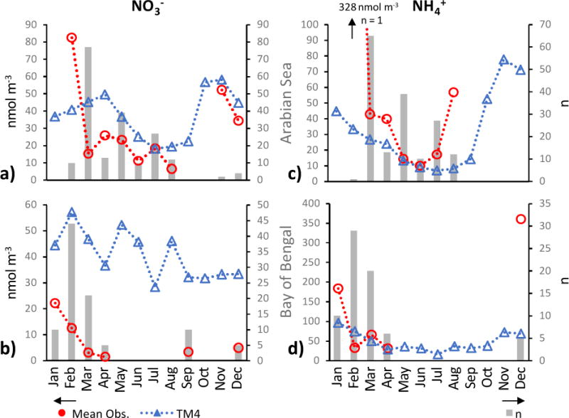
Monthly mean observed aerosol concentrations (red circles), simulated concentrations from TM4 (blue triangles)) and total number of observations (n) in each month (bars) for NO₃⁻ (left) and NH₄⁺ (right) for the Arabian Sea (a & c) and Bay of Bengal (b & d).

Thus, it seems very likely that seasonality contributed to divergence between the models and observations over the NInd region for NH₄⁺, but was less important for NO₃⁻ there. (Note that these analyses of seasonality at the regional-scale allow investigation of the model – observation comparison, but cannot provide assurance that either the ship-based observations, or the model, reproduce accurately the annual mean aerosol concentrations, especially in the NInd region, where there are no independent seasonal records available).

4.4 Role of mineral dust in modifying N deposition fluxes

It is not entirely coincidental that all three of the study regions examined in this paper are impacted strongly by transport and deposition of mineral dust. Interest in the impact of dust deposition on marine productivity (Jickells et al., 2005) has stimulated a great deal of research into aerosol chemistry at the outflows of the world’s major deserts over the past few decades (e.g. Gao et al., 2007; Baker et al., 2013; Srinivas and Sarin, 2013b; Srinivas et al., 2014; Powell et al., 2015). Much of the observational work on dust has generated data on aerosol N concentrations, augmenting the data available in these regions, but the presence of dust adds extra complexity to the comparison performed here. Uptake of nitric acid onto suspended mineral dust particles alters the size distribution and deposition velocity of aerosol nitrate, as well as changing the gas-phase composition of N (Hanisch and Crowley, 2001; Rubasinghege and Grassian, 2009). Atmospheric chemical-transport models for N must therefore also incorporate effective simulations of mineral dust. This is itself a considerable challenge. Dust emissions in TM4, simulated for the year 2008 using ECMWF meteorology, were 1181 Tg yr⁻¹ (Myriokefalitakis et al., 2016), while Kanakidou et al. (2016) simulated emissions almost 30% higher for the year 2005. In the case of ACCMIP, not all of the models involved included simulations of mineral dust aerosols (Lamarque et al., 2013b). In general, modelled dust deposition fluxes to remote ocean regions have been shown to vary by factors of 10 or more (Huneeus et al., 2011; Schulz et al., 2012) and to not reproduce key aspects of the dust cycle even in well-characterised regions (Prospero et al., 2010).

4.5 Challenges posed by uncertainty in dry deposition velocities

As noted above, dry deposition velocities are probably the largest sources of uncertainty in estimates of dry deposition fluxes of aerosol components. Thus the comparisons of observed and modelled aerosol concentrations presented in Fig. 4 – 6 are preferable to comparisons of dry deposition flux because they avoid the uncertainty associated with conversion of measured aerosol concentrations into CalDep. However, modelled aerosol concentrations at a given location are dependent on the parameterisation of dry deposition velocity (together with a number of other factors of varying degrees of uncertainty) applied by the model all along the simulated aerosol transport pathway. Uncertainty in modelled v_d therefore also impacts the effectiveness of the concentration comparison, although gross errors in v_d in models are unlikely to result in good agreement between observed and simulated aerosol concentrations.

5 Summary and Conclusions

A unique dataset of particulate NO₃⁻ and NH₄⁺ concentrations in the marine atmosphere was compiled, based on 2890 samples from oceanographic cruises between 1995 and 2012. The data were mapped to 5° × 5° grid cells and annual average concentrations were calculated for each cell. Dry deposition fluxes for each cell were calculated from these average concentrations. Gridded concentrations and calculated dry deposition fluxes were compared with two different model products: The ACCMIP multi-model mean products of NO_y and NH_x dry deposition, and the TM4 model of NO_y and NH_x deposition fluxes and NO₃⁻ and NH₄⁺ aerosol concentrations and deposition fluxes.

Comparisons of deposition fluxes of NO_y and NH_x from the ACCMIP MMM product and from TM4 with observation-derived fluxes (CalDep) show similar performances for both products, with significant over-estimation of the lower levels of observed NH₄⁺ deposition fluxes. ModDep of NO₃⁻ and NH₄⁺ from TM4 show much better agreement with CalDep than did NO_y and NH_x, which is consistent with significant contributions of gaseous deposition to NO_y and NH_x deposition fluxes.

Given the uncertainties involved in the observations and modelling, it may be that the large scatter in the observation – model comparisons (Figs. 4, 7 and S5) are the best that can be achieved currently in this type of comparison. Uncertainties in dry deposition velocities remain a serious obstacle to improving observation- and modelling-based estimates of the atmospheric flux of material into the ocean. For example, if a given observation of aerosol NO₃⁻ concentration leads to a value of CalDep of 0.1 mg N m⁻² d⁻¹, that value represents, at best, a flux in the range of 0.05 – 0.2 mg N m⁻² d⁻¹. When considering modelled dry N deposition, the uncertainty in v_d (when compounded with the other sources of uncertainty in the modelling) probably implies that fluxes can be estimated to within no better than an order of magnitude. The uncertainty in modelled dry deposition, in turn, leads to uncertainty in modelled wet deposition estimates. This limitation has consequences for the usefulness of models in predicting the impacts of N deposition fluxes on the ocean, both in the present and into the future (Duce et al., 2008; Jickells et al., 2017). Understanding of the dry deposition of particulate matter to the ocean surface has not advanced for several decades (Slinn and Slinn, 1980) and concerted community action is required if further progress is to be made.

There are a number of steps that can be taken to improve model predictions of atmospheric N inputs to the ocean. Observations of N deposition that target key areas of uncertainty (such as regions with strong seasonal cycles; intense gradients in N concentrations/deposition; and with contrasting mineral dust regimes) are required and these field campaigns should include measurements that address the needs of the modelling community. Examples of such measurements include: gas-phase N speciation and deposition flux, in addition to particulate N speciation (in order to better constrain modelled N simulations); more detailed measurement of N species aerosol particle size distributions and measurement of aerosol particle deposition fluxes over the ocean (to help improve estimates of particulate N dry deposition over the ocean); long-term measurement of dry particulate deposition N species fluxes, concurrently with N species wet deposition measurements, at suitable remote island locations. In the future, reducing uncertainties in v_d from small-scale wind and aerosol property heterogeneity may help provide more certain v_d estimates. One way to do so might be to estimate larger-scale v_d from remote sensing observations, based on relationships between N concentrations and surface and remotely-sensed aerosol properties. To date, these relationships are still poorly constrained. Improvements in emissions estimates, such as through the use of satellite-derived fire radiative power to assess biomass burning emissions (Freeborn et al., 2014), are key to improvements in the performance of models. Most model simulations of marine NH₃ emissions are based on the very old inventory of Bouwman et al. (1997). Both observations and models of air – sea NH₃ exchange have progressed since that study (e.g. Johnson et al., 2008; Paulot et al., 2015) and these advances should be incorporated into N atmospheric chemistry transport models more widely. Organic N species have been shown to comprise a significant fraction of atmospheric N (Jickells et al., 2013). Explicit inclusion of organic N into models (e.g. Kanakidou et al., 2012) should therefore result in more effective simulations of the atmospheric N cycle. Future model – observation comparisons would be more effective were the observations compared directly to the corresponding absolute time in the model, rather than over time-averaged periods as done here. Ideally, sampling of comparative values from the models should be done over time intervals matched to the collection period of the observations.

The approach to assessing the performance of N deposition models used here has some obvious limitations. It does, however, offer additional benefits to those provided by comparison to land-based wet deposition networks, in terms of both increasing the geographical distribution of comparative data and in extending the comparison to dry deposition. In the case of N deposition to the ocean, it is very unlikely that a coherent geographically-dispersed database of wet deposition observations will ever be available for this purpose. It is recommended strongly that future model validation and intercomparison exercises should incorporate comparisons to directly-measured aerosol concentrations, rather than to calculated dry deposition fluxes, which are currently subject to large uncertainties. Reporting of surface-level aerosol concentrations should therefore be considered a core requirement for future model intercomparison exercises.

References

- Baker AR, Lesworth T, Adams C, Jickells TD, Ganzeveld L. Estimation of atmospheric nutrient inputs to the Atlantic Ocean from 50°N to 50°S based on large-scale field sampling: Fixed nitrogen and dry deposition of phosphorus. Global Biogeochemical Cycles. 2010;24:GB3006. doi: 10.1029/2009GB003634. [DOI] [Google Scholar]
- Baker AR, Adams C, Bell TG, Jickells TD, Ganzeveld L. Estimation of atmospheric nutrient inputs to the Atlantic Ocean from 50°N to 50°S based on large-scale field sampling: Iron and other dust-associated elements. Global Biogeochemical Cycles. 2013;27:755–767. doi: 10.1002/gbc.20062. [DOI] [Google Scholar]
- Baker AR, Thomas M, Bange HW, Plasencia Sánchez E. Soluble trace metals in aerosols over the tropical south-east Pacific offshore of Peru. Biogeosciences. 2016;13:817–825. doi: 10.5194/bg-13-817-2016. [DOI] [Google Scholar]
- Bauer P, Thorpe A, Brunet G. The quiet revolution of numerical weather prediction. Nature. 2015;525:47–55. doi: 10.1038/nature14956. [DOI] [PubMed] [Google Scholar]
- Bouwman AF, Lee DS, Asman WAH, Dentener FJ, VanderHoek KW, Olivier JGJ. A global high-resolution emission inventory for ammonia. Global Biogeochemical Cycles. 1997;11:561–587. [Google Scholar]
- Buck CS, Landing WM, Resing J. Pacific Ocean aerosols: Deposition and solubility of iron, aluminum, and other trace elements. Marine Chemistry. 2013;157:117–130. doi: 10.1016/j.marchem.2013.09.005. [DOI] [Google Scholar]
- Chien CT, Mackey KRM, Dutkiewicz S, Mahowald NM, Prospero JM, Paytan A. Effects of African dust deposition on phytoplankton in the western tropical Atlantic Ocean off Barbados. Global Biogeochemical Cycles. 2016;30:716–734. doi: 10.1002/2015GB005334. [DOI] [Google Scholar]
- Chung CC, Chang J, Gong GC, Hsu SC, Chiang KP, Liao CW. Effects of Asian Dust Storms on Synechococcus populations in the subtropical Kuroshio Current. Marine Biotechnology. 2011;13:751–763. doi: 10.1007/s10126-010-9336-5. [DOI] [PubMed] [Google Scholar]
- Daskalakis N, Myriokefalitakis S, Kanakidou M. Sensitivity of tropospheric loads and lifetimes of short lived pollutants to fire emissions. Atmospheric Chemistry and Physics. 2015;15:3543–3563. doi: 10.5194/acp-15-3543-2015. [DOI] [Google Scholar]
- Dentener F, Drevet J, Lamarque JF, Bey I, Eickhout B, Fiore AM, Hauglustaine D, Horowitz LW, Krol M, Kulshrestha UC, Lawrence M, Galy-Lacaux C, Rast S, Shindell D, Stevenson D, van Noije T, Atherton C, Bell N, Bergman, Butler T, Cofala J, Collins B, Doherty R, Ellingsen K, Galloway J, Gauss M, Montanaro V, Muller JF, Pitari G, Rodriguez J, Sanderson M, Solmon F, Strahan S, Schultz M, Sudo K, Szopa S, Wild O. Nitrogen and sulfur deposition on regional and global scales: A multimodel evaluation. Global Biogeochemical Cycles. 2006;20:GB4003. doi: 10.1029/2005GB002672. [DOI] [Google Scholar]
- Duce RA, Liss PS, Merrill JT, Atlas EL, Buat-Menard P, Hicks BB, Miller JM, Prospero JM, Arimoto R, Church TM, Ellis W, Galloway JN, Hansen L, Jickells TD, Knap AH, Reinhardt KH, Schneider B, Soudine A, Tokos JJ, Tsunogai S, Wollast R, Zhou M. The atmospheric input of trace species to the world ocean. Global Biogeochemical Cycles. 1991;5:193–259. doi: 10.1029/91GB01778. [DOI] [Google Scholar]
- Duce RA, La Roche J, Altieri K, Arrigo KR, Baker AR, Capone DG, Cornell S, Dentener F, Galloway J, Ganeshram RS, Geider RJ, Jickells T, Kuypers MM, Langlois R, Liss PS, Liu SM, Middleburg JJ, Moore CM, Nickovic S, Oschlies A, Pedersen T, Prospero J, Schlitzer R, Seitzinger S, Sorensen LL, Uematsu M, Ulloa O, Voss M, Ward B, Zamora L. Impacts of atmospheric anthropogenic nitrogen on the open ocean. Science. 2008;320:893–897. doi: 10.1126/science.1150369. [DOI] [PubMed] [Google Scholar]
- Fomba KW, Müller K, van Pinxteren D, Poulain L, van Pinxteren M, Herrmann H. Long-term chemical characterization of tropical and marine aerosols at the Cape Verde Atmospheric Observatory (CVAO) from 2007 to 2011. Atmospheric Chemistry and Physics. 2014;14:8883–8904. doi: 10.5194/acp-14-8883-2014. [DOI] [Google Scholar]
- Fountoukis C, Nenes A. ISORROPIA II: a computationally efficient thermodynamic equilibrium model for K+-Ca2+-Mg2+-NH4+-Na+ -SO42− - NO3−-Cl−-H2O aerosols. Atmospheric Chemistry and Physics. 2007;7:4639–4659. [Google Scholar]
- Freeborn PH, Wooster MJ, Roy DP, Cochrane MA. Quantification of MODIS fire radiative power (FRP) measurement uncertainty for use in satellite-based active fire characterization and biomass burning estimation. Geophysical Research Letters. 2014;41:1988–1994. doi: 10.1002/2013GL059086. [DOI] [Google Scholar]
- Galloway JN, Dentener FJ, Capone DG, Boyer EW, Howarth RW, Seitzinger SP, Asner GP, Cleveland CC, Green PA, Holland EA, Karl DM, Michaels AF, Porter JH, Townsend AR, Vorosmarty CJ. Nitrogen cycles: past, present, and future. Biogeochemistry. 2004;70:153–226. [Google Scholar]
- Galloway JN, Townsend AR, Erisman JW, Bekunda M, Cai Z, Freney JR, Martinelli LA, Seitzinger SP, Sutton MA. Transformations of the nitrogen cycle: Recent trends, questions, and potential solutions. Science. 2008;320:889–892. doi: 10.1126/science.1136674. [DOI] [PubMed] [Google Scholar]
- Ganzeveld L, Lelieveld J, Roelofs GJ. A dry deposition parameterization of sulfur oxides in a chemistry and general circulation. Journal of Geophysical Research-Atmospheres. 1998;103:5679–5694. [Google Scholar]
- Gao Y, Anderson JR, Hua X. Dust characteristics over the North Pacific observed through shipboard measurements during the ACE-Asia experiment. Atmospheric Environment. 2007;41:7907–7922. [Google Scholar]
- Hanisch F, Crowley JN. Heterogeneous reactivity of gaseous nitric acid on Al2O3, CaCO3, and atmospheric dust samples: A Knudsen cell study. Journal of Physical Chemistry A. 2001;105:3096–3106. [Google Scholar]
- Hsu SC, Lee CSL, Huh CA, Shaheen R, Lin FJ, Liu SC, Liang MC, Tao J. Ammonium deficiency caused by heterogeneous reactions during a super Asian dust episode. J Geophys Res. 2014;119:6803–6817. doi: 10.1002/2013JD021096. [DOI] [Google Scholar]
- Huneeus N, Schulz M, Balkanski Y, Griesfeller J, Prospero J, Kinne S, Bauer S, Boucher O, Chin M, Dentener F, Diehl T, Easter R, Fillmore D, Ghan S, Ginoux P, Grini A, Horowitz L, Koch D, Krol MC, Landing W, Liu X, Mahowald N, Miller R, Morcrette JJ, Myhre G, Penner J, Perlwitz J, Stier P, Takemura T, Zender CS. Global dust model intercomparison in AeroCom phase I. Atmospheric Chemistry and Physics. 2011;11:7781–7816. doi: 10.5194/acp-11-7781-2011. [DOI] [Google Scholar]
- Jickells T, Baker AR, Cape JN, Cornell SE, Nemitz E. The cycling of organic nitrogen through the atmosphere. Philosophical Transactions of the Royal Society of London Series B-Biological Sciences. 2013;368:20130115. doi: 10.1098/rstb.2013.0115. [DOI] [PMC free article] [PubMed] [Google Scholar]
- Jickells TD, An ZS, Anderson KK, Baker AR, Bergametti G, Brooks N, Cao JJ, Boyd PW, Duce RA, Hunter KA, Kawahata H, Kubilay N, La Roche J, Liss PS, Mahowald N, Prospero JM, Ridgwell AJ, Tegen I, Torres R. Global Iron Connections between desert dust, ocean biogeochemistry and climate. Science. 2005;308:67–71. doi: 10.1126/science.1105959. [DOI] [PubMed] [Google Scholar]
- Jickells TD, Buitenhuis ET, Altieri K, Baker AR, Capone D, Duce RA, Dentener F, Fennel K, Kanakidou M, LaRoche J, Lee K, Liss PS, Middelburg JJ, Moore JK, Okin G, Oschlies A, Sarin M, Seitzinger S, Sharples J, Singh A, Suntharalingam P, Uematsu M, Zamora LM. A re-evaluation of the magnitude and impacts of anthropogenic atmospheric nitrogen inputs on the ocean. Global Biogeochemical Cycles. 2017;31 doi: 10.1002/2016GB005586. [DOI] [Google Scholar]
- Johnson MT, Liss PS, Bell TG, Lesworth TJ, Baker AR, Hind AJ, Jickells TD, Biswas KF, Woodward EMS, Gibb SW. Field observations of the ocean-atmosphere exchange of ammonia: fundamental importance of temperature as revealed by a comparison of high and low latitudes. Global Biogeochemical Cycles. 2008;22:GB1019. doi: 10.1029/2007GB003039. [DOI] [Google Scholar]
- Kanakidou M, Duce R, Prospero JM, Baker AR, Benitez-Nelson C, Dentener FJ, Hunter KA, Liss PS, Mahowald N, Okin GS, Sarin M, Tsigaridis K, Uematsu M, Zamora LM, Zhu T. Atmospheric fluxes of organic N and P to the global ocean. Global Biogeochemical Cycles. 2012;26:GB3026. doi: 10.1029/2011GB004277. [DOI] [Google Scholar]
- Kanakidou M, Myriokefalitakis S, Daskalakis N, Fanourgakis G, Nenes A, Baker AR, Tsigaridis K, Mihalopoulos N. Past, present and future atmospheric nitrogen deposition. Journal of Atmospheric Sciences. 2016;73:2039–2047. doi: 10.1175/JAS-D-15-0278.1. [DOI] [PMC free article] [PubMed] [Google Scholar]
- Karydis VA, Tsimpidi AP, Pozzer A, Astitha M, Lelieveld J. Effects of mineral dust on global atmospheric nitrate concentrations. Atmospheric Chemistry and Physics. 2016;16:1491–1509. doi: 10.5194/acp-16-1491-2016. [DOI] [Google Scholar]
- Keck L, Wittmaack K. Laboratory studies on the retention of nitric acid, hydrochloric acid and ammonia on aerosol filters. Atmospheric Environment. 2005;39:2157–2162. doi: 10.1016/j.atmosenv.2004.12.021. [DOI] [Google Scholar]
- Keene WC, Galloway JN, Likens GE, Deviney FA, Mikkelsen KN, Moody JL, Maben JR. Atmospheric wet deposition in remote regions: Benchmarks for environmental change. Journal of the Atmospheric Sciences. 2015;72:2947–2978. doi: 10.1175/JAS-D-14-0378.1. [DOI] [Google Scholar]
- Kim TW, Lee K, Najjar RG, Jeong HD, Jeong HJ. Increasing N Abundance in the Northwestern Pacific Ocean Due to Atmospheric Nitrogen Deposition. Science. 2011;334:505–509. doi: 10.1126/science.1206583. [DOI] [PubMed] [Google Scholar]
- Krishnamurthy A, Moore JK, Mahowald N, Luo C, Zender CS. Impacts of atmospheric nutrient inputs on marine biogeochemistry. Journal of Geophysical Research-Biogeosciences. 2010;115:G01006. doi: 10.1029/2009jg001115. [DOI] [Google Scholar]
- Lamarque JF, Dentener F, McConnell J, Ro CU, Shaw M, Vet R, Bergmann D, Cameron-Smith P, Dalsoren S, Doherty R, Faluvegi G, Ghan SJ, Josse B, Lee YH, MacKenzie IA, Plummer D, Shindell DT, Skeie RB, Stevenson DS, Strode S, Zeng G, Curran M, Dahl-Jensen D, Das S, Fritzsche D, Nolan M. Multi-model mean nitrogen and sulfur deposition from the Atmospheric Chemistry and Climate Model Intercomparison Project (ACCMIP): evaluation of historical and projected future changes. Atmospheric Chemistry and Physics. 2013a;13:7997–8018. doi: 10.5194/acp-13-7997-2013. [DOI] [Google Scholar]
- Lamarque JF, Shindell DT, Josse B, Young PJ, Cionni I, Eyring V, Bergmann D, Cameron-Smith P, Collins WJ, Doherty R, Dalsoren S, Faluvegi G, Folberth G, Ghan SJ, Horowitz LW, Lee YH, MacKenzie IA, Nagashima T, Naik V, Plummer D, Righi M, Rumbold ST, Schulz M, Skeie RB, Stevenson DS, Strode S, Sudo K, Szopa S, Voulgarakis A, Zeng G. The Atmospheric Chemistry and Climate Model Intercomparison Project (ACCMIP): overview and description of models, simulations and climate diagnostics. Geosci Model Dev. 2013b;6:179–206. doi: 10.5194/gmd-6-179-2013. [DOI] [Google Scholar]
- Landolfi A, Dietze H, Koeve W, Oschlies A. Overlooked runaway feedback in the marine nitrogen cycle: the vicious cycle. Biogeosciences. 2013;10:1351–1363. doi: 10.5194/bg-10-1351-2013. [DOI] [Google Scholar]
- Markaki Z, Oikonomou K, Kocak M, Kouvarakis G, Chaniotaki A, Kubilay N, Mihalopoulos N. Atmospheric deposition of inorganic phosphorus in the Levantine Basin, eastern Mediterranean: Spatial and temporal variability and its role in seawater productivity. Limnology and Oceanography. 2003;48:1557–1568. [Google Scholar]
- Marple VA, Rubow KL, Behm SM. A microorifice uniform deposit impactor (MOUDI) - description, calibration, and use. Aerosol Science and Technology. 1991;14:434–446. doi: 10.1080/02786829108959504. [DOI] [Google Scholar]
- Morton P, Landing WM, Hsu SC, Milne A, Aguilar-Islas AM, Baker AR, Bowie AR, Buck CS, Gao Y, Gichuki S, Hastings M, Hatta M, Johansen AM, Losno R, Mead C, Patey MD, Swarr G, Vandermark A, Zamora LM. Methods for sampling and analysis of marine aerosols: results from the 2008 GEOTRACES aerosol intercalibration experiment. Limnology and Oceanography-Methods. 2013;11:62–78. doi: 10.4319/lom.2013.11.62. [DOI] [Google Scholar]
- Mourino-Carballido B, Pahlow M, Oschlies A. High sensitivity of ultra-oligotrophic marine ecosystems to atmospheric nitrogen deposition. Geophysical Research Letters. 2012;39:L05601. doi: 10.1029/2011gl050606. [DOI] [Google Scholar]
- Myriokefalitakis S, Daskalakis N, Mihalopoulos N, Baker AR, Nenes A, Kanakidou M. Changes in dissolved iron deposition to the oceans driven by human activity: a 3-D global modelling study. Biogeosciences. 2015;12:3973–3992. doi: 10.5194/bg-12-3973-2015. [DOI] [Google Scholar]
- Myriokefalitakis S, Nenes A, Baker AR, Mihalopoulos N, Kanakidou M. Bioavailable atmospheric phosphorous supply to the global ocean: a 3-D global modelling study. Biogeosciences. 2016;13:6519–6543. doi: 10.5194/bg-13-6519-2016. [DOI] [Google Scholar]
- Paulot F, Jacob DJ, Johnson M, Bell TG, Baker AR, Keene WC, Lima ID, Doney SC, Stock CA. Global oceanic emission of ammonia: constraints from seawater and atmospheric observations. Global Biogeochemical Cycles. 2015;29:1165–1178. doi: 10.1002/2015GB005106. [DOI] [Google Scholar]
- Powell CF, Baker AR, Jickells TD, Bange HW, Chance R, Yodle C. Estimation of the atmospheric flux of nutrients and trace metals to the eastern tropical North Atlantic Ocean. Journal of the Atmospheric Sciences of the American Meteorological Society. 2015;72:4029–4045. doi: 10.1175/JAS-D-15-0011.1. [DOI] [Google Scholar]
- Prospero JM, Landing WM, Schulz M. African dust deposition to Florida: Temporal and spatial variability and comparisons to models. J Geophys Res. 2010;115:D13304. doi: 10.1029/2009JD012773. [DOI] [Google Scholar]
- Pryor SC, Sorensen LL. Dry deposition of reactive nitrogen to marine environments: recent advances and remaining uncertainties. Marine Pollution Bulletin. 2002;44:1336–1340. doi: 10.1016/s0025-326x(02)00234-5. [DOI] [PubMed] [Google Scholar]
- Rubasinghege G, Grassian VH. Photochemistry of adsorbed nitrate on aluminum oxide particle surfaces. Journal of Physical Chemistry A. 2009;113:7818–7825. doi: 10.1021/jp902252s. [DOI] [PubMed] [Google Scholar]
- Schulz M, Prospero JM, Baker AR, Dentener F, Ickes L, Liss PS, Mahowald NM, Nickovic S, Perez Garcia-Pando C, Rodriguez S, Sarin M, Tegen I, Duce RA. The atmospheric transport and deposition of mineral dust to the ocean - Implications for research needs. Environmental Science & Technology. 2012;46:10390–10404. doi: 10.1021/es300073u. [DOI] [PubMed] [Google Scholar]
- Shi JH, Gao HW, Zhang J, Tan SC, Ren JL, Liu CG, Liu Y, Yao XH. Examination of causative link between a spring bloom and dry/wet deposition of Asian dust in the Yellow Sea, China. Journal of Geophysical Research-Atmospheres. 2012;117:D17304. doi: 10.1029/2012jd017983. [DOI] [Google Scholar]
- Singh A, Gandhi N, Ramesh R. Contribution of atmospheric nitrogen deposition to new production in the nitrogen limited photic zone of the northern Indian Ocean. Journal of Geophysical Research-Oceans. 2012;117:C06004. doi: 10.1029/2011jc007737. [DOI] [Google Scholar]
- Slinn SA, Slinn WGN. Predictions for particle deposition on natural waters. Atmospheric Environment. 1980;14:1013–1016. [Google Scholar]
- Somes CJ, Landolfi A, Koeve W, Oschlies A. Limited impact of atmospheric nitrogen deposition on marine productivity due to biogeochemical feedbacks in a global ocean model. Geophysical Research Letters. 2016;43:4500–4509. doi: 10.1002/2016gl068335. [DOI] [Google Scholar]
- Srinivas B, Sarin MM. Atmospheric dry-deposition of mineral dust and anthropogenic trace metals to the Bay of Bengal. Journal of Marine Systems. 2013a;126:56–68. doi: 10.1016/j.jmarsys.2012.11.004. [DOI] [Google Scholar]
- Srinivas B, Sarin MM. Atmospheric deposition of N, P and Fe to the Northern Indian Ocean: Implications to C- and N-fixation. Science of the Total Environment. 2013b;456–457:104–114. doi: 10.1016/j.scitotenv.2013.03.068. [DOI] [PubMed] [Google Scholar]
- Srinivas B, Sarin MM, Rengarajan R. Atmospheric transport of mineral dust from the Indo-Gangetic Plain: Temporal variability, acid processing, and iron solubility. Geochemistry Geophysics Geosystems. 2014;15:3226–3243. doi: 10.1002/2014gc005395. [DOI] [Google Scholar]
- Suntharalingam P, Buitenhuis E, Le Quere C, Dentener F, Nevison C, Butler JH, Bange HW, Forster G. Quantifying the impact of anthropogenic nitrogen deposition on oceanic nitrous oxide. Geophysical Research Letters. 2012;39:L07605. doi: 10.1029/2011gl050778. [DOI] [Google Scholar]
- Vet R, Artz RS, Carou S, Shaw M, Ro CU, Aas W, Baker A, Bowersox VC, Dentener F, Galy-Lacaux C, Hou A, Pienaar JJ, Gillett R, Forti MC, Gromov S, Hara H, Khodzher T, Mahowald NM, Nickovic S, Rao PSP, Reid NW. A global assessment of precipitation chemistry and deposition of sulfur, nitrogen, sea salt, base cations, organic acids, acidity and pH, and phosphorus. Atmospheric Environment. 2014;93:3–100. doi: 10.1016/j.atmosenv.2013.10.060. [DOI] [Google Scholar]
- Wang R, Balkanski Y, Bopp L, Aumont O, Boucher O, Ciais P, Gehlen M, Peñuelas J, Ethé C, Hauglustaine D, Li B, Liu J, Zhou F, Tao S. Influence of anthropogenic aerosol deposition on the relationship between oceanic productivity and warming. Geophysical Research Letters. 2015;42:10745–10754. doi: 10.1002/2015GL066753. [DOI] [PMC free article] [PubMed] [Google Scholar]
- Young AH, Keene WC, Pszenny AAP, Sander R, Thornton JA, Riedel TP, Maben JR. Phase partitioning of soluble trace gases with size-resolved aerosols in near-surface continental air over northern Colorado, USA, during winter. J Geophys Res. 2013;118:9414–9427. doi: 10.1002/jgrd.50655. [DOI] [Google Scholar]
- Zamora LM, Landolfi A, Oschlies A, Hansell DA, Dietze H, Dentener F. Atmospheric deposition of nutrients and excess N formation in the North Atlantic. Biogeosciences. 2010;7:777–793. [Google Scholar]
Associated Data
This section collects any data citations, data availability statements, or supplementary materials included in this article.