Can increased spatial resolution solve the crossing fiber problem for diffusion MRI?

Abstract

It is now widely recognized that voxels with crossing fibers or complex geometrical configurations present a challenge for diffusion MRI (dMRI) reconstruction and fiber tracking, as well as microstructural modeling of brain tissues. This “crossing fiber” problem has been estimated to affect anywhere from 30% to as much as 90% of white matter voxels, and it is often assumed that increasing spatial resolution will decrease the prevalence of voxels containing multiple fiber populations. The aim of this study is to estimate the extent of the crossing fiber problem as we continually increase the spatial resolution, with the goal of determining whether it is possible to mitigate this problem with higher resolution spatial sampling. This is accomplished using ex vivo MRI data of the macaque brain, followed by histological analysis of the same specimen to validate these measurements, as well as to extend this analysis to resolutions not yet achievable in practice with MRI. In both dMRI and histology, we find unexpected results: the prevalence of crossing fibers increases as we increase spatial resolution. The problem of crossing fibers appears to be a fundamental limitation of dMRI associated with the complexity of brain tissue, rather than a technical problem that can be overcome with advances such as higher fields and stronger gradients.

Graphical Abstract

Using diffusion MRI and subsequent histological analysis, we estimate the extent of the “crossing fiber” problem as we continually increase spatial resolution. Our results indicate that the prevalence of crossing fibers actually increases as we increase spatial resolution. The problem of crossing fibers appears to be a fundamental limitation of diffusion MRI associated with the complexity of brain tissue, rather than a technical problem that can be overcome with advances such as higher fields and stronger gradients.

1. Introduction

Diffusion-weighted magnetic resonance imaging (dMRI) is a technique sensitive to the random thermal motion of water (1), providing contrasts that give unique insights into tissue architecture. In the neuroimaging community, dMRI research can loosely be divided into two main classes (2). The first concerns mapping the neural fiber pathways, or connectivity, of the brain. These fiber “tractography” techniques exploit diffusion anisotropy to infer the orientation of the underlying white matter (WM) in each voxel, and use the field of these discrete orientation estimates to reconstruct continuous trajectories called streamlines (for review, see (3)). The second class concerns mapping microstructural properties of the tissue. Rather than focusing on fiber orientation estimation, these techniques attempt to extract properties such as axon diameter, axon density, or degree of myelination – measures serving as biomarkers for WM and gray matter (GM) physiology and pathology. Despite significant progress in assessing microstructure and connectivity, both areas of research are complicated when voxels contain complex fiber configurations, an issue that has generically been referred to as the “crossing fiber problem” (2,4,5).

This crossing fiber problem typically refers to the situation when there are two or more differently oriented fiber bundles located in the same dMRI imaging voxel (4,5). This causes a partial volume effect, with multiple fiber bundles contributing to the dMRI signal. In general, this partial volume effect can occur in any situation where axons within a voxel do not all run parallel to each other. Therefore, the ‘crossing fiber’ problem encompasses not only crossing fibers, but also fibers of bending, fanning, or kissing geometries.

It is now widely recognized that these geometries can lead to ambiguous or incorrect estimates of fiber orientation (6–8) and subsequent failure of tractography (9,10), as well as misleading microstructural indices. This is particularly true for one of the earliest, yet arguably the most common, dMRI technique, diffusion tensor imaging (DTI) (11), which models a single primary fiber direction per voxel. While a plethora of methods have been introduced to resolve crossing fibers for tractography (7,12–17), they are still plagued by assumptions on the signal, lengthy acquisition requirements, and limited ability to resolve fibers crossing at acute angles. Similarly, methods have been introduced to describe axon diameters, dispersion, and density (18–24), but typically assume a single known orientation of axons in the model, limiting their use to small regions of the brain with known orientation, or leading to ambiguous measurements in crossings between tracts with different orientations.

Given its implications on dMRI neuroimaging studies, it is important to fully investigate the scope of the crossing fiber problem. With axon diameters on the order of microns (25), fiber tracts (i.e., bundles of axons) often less than a few millimeters wide, and dMRI voxels typically 2–3 mm in each dimension on clinical scanners, it is not unreasonable to expect crossing fibers to be widespread throughout the brain. In fact, fitting dMRI data to multiple tensors, Behrens et al. (9) found that nearly one-third of voxels contain 2 fiber populations. Moreover, using data acquisition and modeling techniques specifically designed to estimate the prevalence of crossing fibers, Jeurissen et al. (26) found that as many as 90% of white matter voxels are affected by crossing fibers. However, these results have yet to be validated through histology. Also, because these results were obtained using dMRI methods designed for detecting discrete sets of fiber orientations, or discrete “peaks” in the fiber orientation distribution (FOD), it is unclear whether these fractions represent true crossing fibers, or something like fiber “spreading” that is interpreted as multiple distinct fiber populations using these dMRI techniques.

It is often assumed that increasing the spatial resolution will decrease the prevalence of voxels containing multiple fiber populations. If true, there would be a tradeoff between minimizing the crossing fiber problem (increasing spatial resolution), and increasing signal-to-noise ratio (SNR), increasing angular resolution (number of diffusion weighted images), and increasing diffusion weighting (or b-value, which has been shown to provide greater sensitivity to fiber orientations). At present, there is little consensus on the optimal acquisition protocol, which is typically determined based on the type of questions to be answered from the data. Moreover, it is unknown what resolution is necessary to ameliorate this crossing fiber problem, or if it is at all feasible with advances in imaging methods in the foreseeable future.

In this study, we set out to estimate the extent of the crossing fiber problem as a function of spatial resolution. Specifically, our goal is to determine whether it is possible to significantly mitigate the crossing fiber problem by increasing spatial resolution. This is performed using both ex vivo MRI data from the macaque brain, followed by histological analysis of the same specimen. Ex vivo dMRI offers several experimental advantageous including longer scanning times and absence of motion, allowing acquisition of data with much higher SNR at a resolution currently unachievable in the clinic. Histological methods allow us to further extend this analysis to resolutions not possible even on pre-clinical scanners. In addition, it serves as a validation of the current standard of MRI techniques for resolving crossing fibers. For dMRI, we report the fraction of crossing fibers in WM and GM, as well as the inter-fiber angle of crossing fibers in each voxel, as a function of acquisition resolution. For histology, we report the fraction of voxels with a “complex” geometry at varying resolution levels. In addition, in direct analogy to dMRI, we report on a subset of these complex voxels – those that exhibit distinct “crossing” fibers. Finally, we also describe the histological inter-fiber angle of these fibers at each resolution level.

2. Methods

2.1 MRI acquisition

All animal procedures were approved by the Vanderbilt University Animal Care and Use Committee. MRI experiments were performed on a single hemisphere of an adult Rhesus Macaque (Macaca Mulatta) brain that had been perfusion fixed with physiological saline followed by 4% paraformaldehyde. The brain was then immersed for 3 weeks in phosphate-buffered saline (PBS) medium with 1mM Gd-DTPA in order to reduce longitudinal relaxation time (27). The brain was placed in liquid Fomblin and scanned on a Varian 9.4 T, 21 cm bore magnet. For WM/GM segmentation, a structural image was acquired using a 3D gradient echo sequence (TR = 50ms; TE = 3ms; flip angle = 45°) at 200um isotropic resolution.

Diffusion data were then acquired with a 3D spin-echo diffusion-weighted EPI sequence (TR = 340ms; TE = 40ms; NSHOTS = 4; NEX = 1; Partial Fourier factor = .75). Diffusion gradient duration and separation were 8ms and 22ms, respectively, and the b-value was set to 6,000 s/mm², which has been shown to be in the optimal range for modeling multiple fiber populations in ex vivo specimens (28). A gradient table of 101 uniformly distributed directions (29) was used to acquire 101 diffusion-weighted volumes with four additional image volumes collected at b=0. This acquisition protocol was performed at imaging resolutions ranging from 800um isotropic to 300um isotropic, in 100um increments. All acquisition parameters were kept constant (including diffusion times), except for the field-of view and the number of phase encoding and readout samples required to achieve the intended resolution. Total acquisition time was approximately 48 hours.

2.2 MRI fiber orientation estimation

Fiber orientations were estimated using constrained spherical deconvolution (CSD) (30), and following the procedures developed and outlined in (26). The diffusion-weighted signal was first deconvolved with the single-fiber response function (14,30), estimated from all WM voxels with an FA > 0.7, to obtain the FOD fit to spherical harmonics of degree 8 (the response function was derived independently for each dataset). A peak-finding procedure was then performed to identify distinct fiber orientations. This algorithm uses a Newton optimization algorithm to identify local maxima of the FOD that meet a specific threshold criterion. As in (26), maxima in the FOD are included if the peak amplitude is >10% of the maximum peak amplitude. The number of unique peaks is then counted and assumed to be equal to the number of fiber populations in each MRI voxel. This procedure was performed in all voxels, for datasets at all acquired resolutions. In this study, we refer to voxels containing >1 discrete peaks as voxels with “crossing fibers”.

2.3 Histology Acquisition

After imaging, the brain was embedded in dry ice and sectioned on a microtome at a thickness of 25um in the coronal plane. Sixteen slices, covering the entire brain, were selected for this study. The selected tissue sections were stained for myelin using the silver staining method of Gallyas (31) and mounted on glass slides. Whole-slide brightfield microscopy was performed using a Leica SCN400 Slide Scanner at 20x magnification, resulting in an in-plane resolution of 0.5um/pixel.

2.4 Histological fiber orientation estimation

The histological fiber orientations were defined on myelin-stained slices using structure tensor (ST) analysis (32–34). ST analysis is an image processing technique based on the dyadic product of the image gradient vector with itself, resulting in an orientation estimate of objects in every pixel in the image. These techniques have previously been performed on histological samples in the brain of rats (33), squirrel monkeys (35), macaques (36), and humans (34,37).

Histological fiber orientation distributions were calculated by combining pixel-wise estimates of orientation over larger volumes of tissue, constructed to match potential MRI voxels. For example, a voxel with a resolution of 32um would be created by combining all orientation estimates in an area with a 32um by 32 um field of view in order to produce that voxels FOD. The FOD in each “voxel” was computed as the histogram of orientation estimates using 64 equally spaced bins, as performed in (34). These FOD’s were then fit to a von Mises distribution (38)

$$f(\theta ;\mu ,\kappa )=\frac{e^{\kappa \text{cos}2(\theta -\mu )}}{2\pi I_0(\kappa )}$$

and a mixture of two von Mises distributions. Here, μ is center of the distribution with concentration parameter κ, and I₀ is the modified Bessel function of order 0. Also note the factor 2 in the exponent, which was included because the orientation distributions in this study are pi-periodic. Both distributions also included an isotropic component. Fitting was performed using the Matlab Curve Fitting Toolbox (The MathWorks, Natick, MA, USA).

Model selection was performed using the Akaike information criterion (AIC) (39). The AIC is a measure of the quality of a given model, and quantifies the trade-off between model complexity and goodness-of-fit:

$$\mathit{AIC}=-2log(L)+2K+\frac{2K(K+1)}{N-K-1}$$

where L is the likelihood of obtaining the data given the current model, K is the number of estimated parameters, and N is the number of measurements (40). The lower the AIC, the more predictive the model is. Thus, the AIC was calculated for both the single and mixture von Mises distributions for each voxel, and the model with the lowest AIC was selected to represent the FOD in that voxel.

We then classified the histological voxels based on model selection and the resulting FOD. If a single von Mises distribution was the best fit, the voxel was classified as a “single fiber” voxel. In this case, the parameter θ reflects the dominant fiber orientation. If a mixture model was the best fit, the voxel was classified as a “complex fiber” voxel. To further classify the complex configuration, we performed a procedure analogous to that for MRI and search for local maxima, or peaks, in the FOD that were >10% of the maximum peak amplitude. If two distinct peaks existed, the voxel was classified as a “crossing fiber” voxel. Thus, “crossing fibers” are a subset of “complex fibers”. Complex fibers that did not contain two distinct peaks in the FOD (i.e. not crossing) could be the result of asymmetric FOD’s due to geometries like fiber fanning or bending (see Discussion). The fiber classifications and definitions for both dMRI and histology are summarized in Table 1.

Table 1.

Fiber classification definitions for MRI and histological analysis.

MRI	Single Fiber	Voxel where FOD derived from CSD has 1 local maximum (1 peak)
	Crossing Fiber	Voxel where FOD derived from CSD has >1 local maximum (>1 discrete peaks)
Histology	Single Fiber	FOD derived from ST Analysis best fit to single von Mises distribution (1 peak)
	Complex Fiber	FOD derived from ST Analysis best fit to mixture of Von Mises distributions
	Crossing Fiber (Crossing ⊆ Complex)	FOD derived from ST Analysis best fit to mixture of Von Mises distributions AND FOD derived from ST Analysis has >1 local maximum (>1 discrete peaks)

For all complex fiber voxels (including crossing fibers), we calculated the inter-fiber angle, or the angle that the parameter θ from the two distributions make with each other. These histological procedures were performed at “voxel” sizes ranging from 32 um isotropic to 1024 um isotropic, doubling the linear dimensions at each step. For both MRI and histological analysis, we present results on WM voxels only, as the crossing “fiber” problem refers specifically to axons in the WM tissue.

3. Results

3.1 Fiber orientation estimation in crossing fiber regions

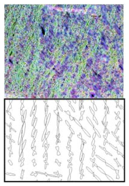
A region of the brain containing crossing fibers of the superior corona radiata (SCR) and the body of the corpus callosum (BCC) is examined in detail in figure 1. A color-coded orientation map at native resolution (Fig. 1A) demonstrates the ability to detect the orientation of individual myelinated fibers in these intersecting fiber bundles. Zooming in on a region of fiber crossings (yellow box), the left-right fibers of the BCC (blue/red) and superior-inferior fibers of the SCR (green/yellow) are intersecting in a woven “checkerboard-like” pattern, highlighting the stereotypical “crossing fiber” problem. Interestingly, even in the BCC (blue box), a region typically assumed to contain a single homogenous fiber population, ST analysis is able to capture a dispersion, or heterogeneity of orientations, on a microscopic scale.

Figure 1.

Fiber orientation estimation in a crossing fiber region. The results of structure tensor analysis on a myelin-stained histological slice shown as a color-coded orientation map (A), is shown zoomed in on two regions containing crossing (yellow box), and disperse (blue box) fibers. The resulting FODs are displayed at varying resolution levels (B). From the resulting FODs, voxels are characterized as crossing fiber (C; green) vs. not-crossing fibers (C; red), as well as single fiber (D; red) vs. complex fibers (D; green), at all resolutions. Note that “not-crossing” voxels are those that with single fiber populations in addition to complex fibers that do not contain two discrete local maxima. Voxels from diffusion MRI in the same region are also displayed as single fiber (E; red) vs. crossing fibers (E; green). Histograms for this specific region of interest show percentages of crossing fibers (F; left) and percentages of complex fibers (F; middle) for histology, as well as percentage of crossing fibers (F; right) for dMRI.

To identify voxels in this region containing crossing or complex fiber configurations, the FODs were fit to a single von Mises and a mixture of von Mises distributions (Fig. 1B) at all resolution levels. At the coarsest resolution (1024um) the predominant white matter tract orientations are visible, even with broad peaks (low κ), and throughout the entire region of intersection. At increasing resolutions levels (256um and 64um) there is still evidence of crossing fibers. The peaks become narrower, yet there is still spatial coherence in peak orientations.

Maps of the types of fiber populations detected in histology (Fig. 1C, D) similarly show a high degree of structural coherence. As the voxel size decreases, there is evidence of crossing fibers in the BCC, whereas at a coarse resolution typical of dMRI, these regions do not contain multiple (distinct) peaks in orientation (Fig. 1C). However, at these coarse resolutions, nearly all voxels suggest a complex geometry (Fig. 1D). The orientations become less complex at the higher spatial resolutions, particularly in the BCC. However, a large percentage of voxels still do not support a simple single fiber geometry. The results of MRI data in the same region show trends qualitatively similar to that of the “crossing” fiber histological analysis; specifically, the BCC is composed of largely single fiber regions, yet, even at the highest spatial resolutions, crossing fibers still persist throughout the region of interest.

Figure 1.F summarizes the results in this region in plot form. From dMRI, the fraction of voxels with crossing fibers in this region increases as the image resolution increases. Similarly, the fraction of histological voxels exhibiting multiple peaks (i.e. crossing fibers) also increases at higher resolutions. Conversely, the histological “complex” fibers decreases as the resolution increases.

3.2 MRI crossing fiber analysis

The prevalence of crossing fibers was determined for all voxels in the WM, at all resolution levels. Maps of the number of fiber populations detected in the WM are shown in Figure 2A. At all spatial scales, large clusters of voxels containing two or more orientations are present throughout the brain. Examples of regions with two fiber populations include the BCC and anterior corona radiata (ACR) (label 1), BCC and ACR (label 2), and posterior thalamic radiation (PTR) and the superior longitudinal fasciculus (SLF) (label 3). Although labeled in the highest resolution dataset, these clusters appear structurally quite similar and of comparable size at all resolutions, although a slight reduction in the area of these crossing fiber regions at more coarse resolutions is discernable. A cluster of 3 fiber populations is shown at the intersection of the posterior corona radiata (PCR), the BCC, and the dorsal posterior corona radiata (DPCR) (label 4). Interestingly, this cluster nearly disappears in the 800 and 700 um datasets.

Figure 2.

(A) Number of fiber orientations per voxel (red: 1, green: 2, blue: 3) estimated using CSD. Numbered arrows highlight regions of crossing fibers and are described in the text. (B) Glyphs highlighting FODs estimated using CSD for voxels at 800 um and 300 um isotropic. Note that background color corresponds to that in (A), while glyph color is based on fiber orientation, where red, green, and blue represent fibers running right/left, anterior/posterior, and superior/inferior.

Figure 2B displays the FOD glyphs that are typical of dMRI, at both the lowest and highest resolution levels. At both resolutions, we see orientation coherence across space in regions containing both single and crossing fibers. However, the 300um glyphs indicate a higher prevalence of voxels with multiple fiber populations (particularly those with 3 peaks), and qualitatively the glyphs appear shaper, with more concentrated orientation distributions.

Figure 3 summarizes the incidence of crossing fibers for all acquired image resolutions. Consistent with the qualitative results of Figure 2, the fraction of crossing fibers increases as the voxel size decreases. Multiple fiber populations were found in 23% of all WM voxels at 800um isotropic resolution, and in 51% at 300um isotropic resolution.

Figure 3.

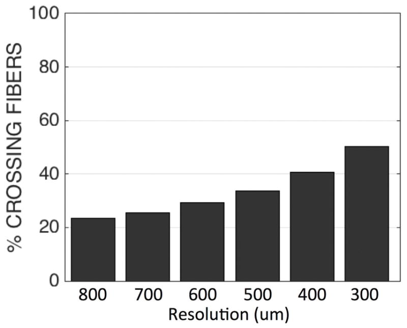
Percentages of crossing fiber voxels throughout the WM as determined using CSD, for different MRI acquisition resolutions.

The inter-fiber angle of all voxels with crossing fibers was investigated, and summarized as histograms in Figure 4. For all cases, a majority of the resolved fiber crossing occurred at nearly orthogonal angles. The 1^st, 2^nd, and 3^rd quartile of crossing angles, in all cases, was in the range of 63–69°, 75–78°, and 83–85%, respectively. Similarly, for all datasets, almost all crossing angles detected (95% of all crossings) are greater than ~47°.

Figure 4.

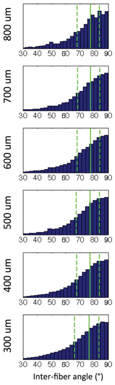
Histograms of inter-fiber angle for crossing fiber voxels in WM, at all acquired dMRI resolutions. The 1^st, 2^nd, and 3^rd quartiles are shown as dashed, solid, and dashed lines, respectively.

3.3 Histological crossing/complex fiber analysis

To validate the dMRI measurements, as well as identify and quantify crossing fibers at resolutions currently unachievable with even preclinical imaging, ST analysis of histological sections was performed for all slices. Visual inspection of maps displaying crossing fibers (Figure 5) shows crossings in regions previously identified in MRI. These regions still show evidence of multiple, distinct fiber bundles down to resolutions of 32um. As in the dMRI data, these maps show spatial coherence, suggesting genuine anatomical features.

Figure 5.

Histological maps of crossing fibers (green) vs. voxels without crossing fibers (red). Crossing fibers are defined as voxels whose FOD contains two distinct local maxima, or peaks. Note that red voxels are those with single fiber populations in addition to complex fibers that do not contain two distinct local maxima

Visual inspection of “complex” fibers (Figure 6) shows that a large majority of the voxels meets this criterion, particularly at lower resolutions. Very few regions meet the definition of a voxel containing only a single fiber bundle. In fact, the only regions in Figure 6 that show large areas without complex fibers are the corpus callosum (label 1), the external capsule (label 2), the SLF III (label 3), and the middle longitudinal fasciculus (label 4). Even these regions become more complex as the spatial resolution decreases towards those currently achievable with dMRI. Further yet, these regions may still contain complex geometries that are unable to be captured using 2D brightfield microscopy, and the number of regions with a single dominant orientation may be overestimated on histology.

Figure 6.

Histological maps of complex fibers (green) and single fibers (red). Complex fibers are defined as voxels whose FOD supports fitting to a mixture of von Mises distributions, and may or may not contain two distinct peaks in the FOD.

Figure 7 quantifies these results in histogram form. These results confirm that, in general, the fraction of voxels with crossing fibers increases at higher resolutionsf. Crossing fibers are most prevalent at 32um resolution, affecting as much as 52% of voxels in the WM. In contrast, the fraction of voxels with complex geometries tends to decrease somewhat at the higher resolutions, leveling off at approximately 128um resolution.

Figure 7.

Percentages of crossing fibers (top) and complex fibers (bottom) throughout WM as determined through ST analysis of histology, for different “voxel” sizes. Error bar shows standard deviation across 16 histological slices.

Figure 8 shows histograms of inter-fiber angles for crossing fibers and complex fibers. For crossing fibers, the histograms shift to the left (toward smaller angles) at the highest resolutions. From coarse to fine resolutions, the median crossing angle decreases from 65° to 29° in the WM. The angular difference between the centers of the two von Mises distributions shows similar trends for the complex distributions, although with much lower angular differences. The median inter-fiber angle is reduced from 37° at 1024um resolution, to 23° at 32um resolution.

Figure 8.

Histograms of inter-fiber angles for crossing fibers (left) and complex fibers (right) in WM, at all resolutions, as determined using ST analysis of histological sections. The 1^st, 2^nd, and 3^rd quartiles are shown as dashed, solid, and dashed lines, respectively.

3.4 Qualitative Analysis

To understand these trends, two more regions (each 1024um across) are further analyzed, including a region with two non-overlapping fiber populations (Figure 9) and one with two interwoven fiber populations (Figure 10). For both figures, the original gray scale image (A) is shown along with the color-coded orientation maps (B). The FOD’s at all resolutions are shown (C), along with fiber classification (D), and (if crossing fibers exist), the crossing angle (E).

Figure 9.

Histological analysis of region with two non-overlapping fiber populations. Structure tensor analysis on myelin-stained region of interest (A) is shown as color-coded orientation map (B). For all spatial resolutions, 2D FODs are displayed (C). Voxels are characterized as single fiber (D; black), complex fibers (D; green), or complex “crossing” fibers (D; yellow). In voxels with crossing fibers, the inter-fiber angle (in degrees) is shown in (E). White oval highlights the interface between the two fiber populations.

Figure 10.

Histological analysis of region with two overlapping fiber populations. Structure tensor analysis on myelin-stained region of interest (A) is shown as color-coded orientation map (B). For all spatial resolutions, 2D FODs are displayed (C). Voxels are characterized as single fiber (D; black), complex fibers (D; green), or complex “crossing” fiber (D; yellow). In voxels with crossing fibers, the inter-fiber angle (in degrees) is shown in (E). Solid box highlights a crossing fiber voxel at 256um resolution. At a coarser spatial resolution (512um), the ability to detect discrete fiber populations is limited by partial volume effects (dashed box).

Figure 9 shows the case of an apparent orthogonal crossing voxel at larger voxel sizes (see Fig 9, C, D, E). As the voxel size decreases, the intersection of the two bundles is highlighted (Fig. 9. E, white oval), where most crossing angles are nearly orthogonal. However, at even higher spatial resolutions, multiple fiber populations are detected in areas not along the interface of the two bundles, and at more acute angles. This is caused by the spatial averaging of incoherent fibers within the same fiber “bundle”. This figure demonstrates that crossing fibers are more prevalent at higher spatial resolutions, and that higher spatial resolutions typically resolve fibers crossing at more acute angles.

Figure 10 shows a fiber geometry typical in many regions of the brain, a so-called “checkerboard-like” crossing. The solid box around an example FOD shows a crossing fiber region. When the four neighboring regions (dashed box) are averaged to go to the next coarser resolution level (i.e. larger voxel size), the ability to distinguish separate fiber populations is lost, and the voxel is now a complex fiber (rather than complex-crossing). This is because the inter-voxel angular dispersion of the individual fiber populations becomes larger than the crossing angle of the two fiber populations, and it blurs the FOD, reducing the ability to resolve discrete peaks. This, again, explains why crossing fiber populations may be more prevalent at higher spatial resolution.

3.5 Crossing Fibers and SNR

The role of SNR on CSD reconstruction has been studied in great detail (30,41), and it is well known that a decreased SNR can results in spurious, false-positive peaks. To examine whether our findings of an increased prevalence of crossing fibers at higher resolution could be due to the comparatively lower SNR, we assess the effects of SNR on our MRI data directly. Gaussian random noise was added in quadrature to the lowest resolution dataset (800 um isotropic) in order to make datasets with equivalent SNR to all other resolutions. The effects of SNR on crossing fibers is shown in Figure 11. As the SNR decreases towards that of the highest resolution dataset, the prevalence of crossing fibers increases from 23% to 29% of all WM voxels. This increase is much smaller than that found for increasing resolution, shown in Fig 3.

Figure 11.

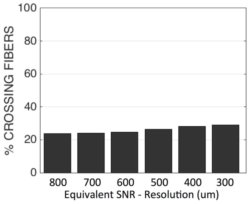
Percentages of crossing fiber voxels throughout the WM determined using CSD, for varying SNR levels. SNR levels were simulated by adding Gaussian random noise in quadrature to all DWIs of the 800um isotropic dataset in order to obtain an SNR equivalent to all other acquired resolutions.

3.6 2D projection of MRI FOD

One discrepancy between MRI and histology is the lower percent of crossing fibers in histology relative to MRI at similar resolutions (for example, compare 512um histology in Figure 9 with 500um MRI in Figure 5). To determine whether this is due to the 2D nature of the histology, we performed a projection of all MRI-derived 3D FOD’s onto the coronal plane, and the same 2D fitting procedures used for histology.

Figure 12 shows the fraction of crossing and complex fibers for the 2D FOD projections in WM. Similar to the results from 3D MRI and 2D histology, these figures show an increase in the fraction of crossing fibers at increasing resolutions. These values are much closer to the results from the 2D histological analysis at similar resolution levels (compare to Figure 7), and confirm that the discrepancy between 3D MRI and 2D histology is largely due to the projection of orientation information into a 2D plane.

Figure 12.

Percentages of crossing fibers (top) and complex fibers (bottom) throughout WM as determined after 2D projection of the CSD FOD, and fitting to a 2D circular distribution (in a manner equivalent to analysis of histological data).

4. Discussion

The aim of this study was to investigate the prevalence of crossing fibers in the brain as the spatial resolution is continually increased. Using both dMRI and subsequent histology, we find that the fraction of voxels with crossing fibers varies with resolution, but in an unintuitive way – the percentage of crossing fibers increases as the resolution increases (Figures 3 and 7). The problem of crossing fibers appears to be a fundamental limitation of dMRI associated with fiber microstructure, rather than a technical problem that can be overcome with higher fields, stronger gradients, or technological advances that may increase spatial resolution. This limitation is likely shared by any imaging method (e.g., polarized light imaging) that is subject to partial volume averaging of fiber orientation information.

One potential explanation for these results could be an artefactual increase in voxels with false-positive peaks caused by a decreased SNR of the high-resolution datasets. While an analysis of SNR-equivalent datasets does show a small increase in WM crossing fibers (Figure 11), this increase is only a small fraction of that due to increased resolution (compare to Figure 3), and the resultant decreased partial volume averaging. It is important to note that even our highest resolution MRI dataset (300um isotropic) had an SNR of ~38 in the WM of the b0 image, a value much higher than is expected in typical human DWIs. Finally, the finding that the prevalence of crossing fibers increases as resolution increases is also validated using histological analysis at spatial scales over a range an order of magnitude greater than the dMRI data.

A surprising result was that even at voxel size as low as 32um on histology, a size much smaller than the scale of WM fiber tracts, crossing fibers are found in >50% of voxels in the WM. So, although there is a much finer delineation of structures, resolutions much higher than currently achievable on pre-clinical scanners still will not eliminate the crossing fiber problem. In fact, our data suggest that with smaller voxels and the consequent finer delineation of structures, there is less partial volume averaging of axon orientations between and within tracts. As voxel size increases, the within-voxel angular dispersion of individual fibers can become larger than the crossing angle of the two fiber populations, which reduces the ability to resolve discrete peaks in the fiber orientation distribution. This implies that the minimum detectable crossing angle depends on both the within-voxel orientation dispersion and the intrinsic angular resolution of the imaging method. Increased spatial resolution leads to less ambiguous orientation estimates in regions containing complicated fiber geometries (fiber dispersion, fiber splaying, fibers crossings at very acute angles), which are eventually resolved into multiple distinct fiber populations at higher spatial resolutions. These results, however, do not imply less accurate fiber tracking at higher resolutions. Because there is less partial volume averaging, and more voxels containing pure crossing fibers, it makes the crossing fiber model more valuable at these resolutions.

While many dMRI techniques are geared towards resolving crossing fibers, histological analysis was able to capture a range of complex fiber geometries. Figure 7 shows that the fraction of fibers containing complex geometries does decrease at higher spatial resolutions, yet remains as high as ~60% at 32um. Our definition of “complex” fibers not only includes voxels with distinct crossing fibers, but also includes any situation where partial volume effects arise between multiple, or even within single, fiber populations. This could include asymmetries in the FOD due to fibers with high curvature or fiber fanning. These complex fibers represent regions where the diffusion tensor (and any metrics derived from it) will fail to accurately capture the underlying fiber distribution, even if the region still contains only a single fiber population. In addition, the regions described by complex, but not crossing fibers, are regions where even methods developed to resolve crossing fibers (7,12–17) may fail to characterize the true tissue complexity, which cannot be adequately described by a simple count of the number of discrete peaks. It is interesting to note that these complex configurations can take place in regions typically assumed to contain single fiber populations (e.g., the corpus callosum), where heterogeneous fiber orientations are apparent in histological sections (see Figure 1).

These results have implications for the future development of dMRI acquisition methods. Because voxels with complex fiber configurations will always exist in datasets, even at resolutions far beyond current dMRI capabilities, it may be more beneficial to focus on appropriate tissue models for describing fiber geometry in voxels rather than focus on pushing resolution (and sacrificing SNR), where the gains in fiber reconstruction accuracy may be minimal. For dMRI sessions, rather than acquiring high spatial resolution data, time may be better spent on acquiring high angular resolution data or more unique diffusion weightings, at a higher SNR, to accommodate biophysical modeling, although specific acquisition requirements are likely to depend on the intended goal of the individual study, in addition to the implemented diffusion reconstruction method Also, because of the pervasiveness of complex fiber configurations, significant emphasis could be placed on models with fiber fanning and curving (42–44), as well as those containing multiple compartments, allowing both fanning and crossing (45).

An interesting discrepancy between MRI and histology is the inter-fiber angle in voxels containing crossing fibers. Figure 4 shows that dMRI tends to resolve crossing fibers when the fibers are crossing at nearly orthogonal angles, at all resolutions. Many dMRI techniques are limited by the minimum angle that can be resolved reliably. While dependent upon acquisition parameters, this minimum resolvable angle is typically in the range of 40–60°. A similar distribution of crossing angles has been previously described (26), and if the observed orthogonal crossings are the result of genuine anatomical structures, they could have significant implications for evolution, development, and brain connectivity (46). However, our results suggest that when voxels are large enough (i.e., when intra-voxel orientation dispersion grows large), then near-orthogonal crossings will be most common. Hence, the ‘blurring’ of FODs (and other orientation distribution functions) due to intra-voxel fiber dispersion biases measurements of the prevalence of orthogonal fiber crossings. Analysis of histological sections (Figure 8) shows that the mode of the inter-fiber angle distribution is much smaller than 90°, and actually decreases at higher spatial resolutions, for both crossing and complex configurations. CSD has an intrinsic angular resolution limit defined by the deconvolution kernel (30), meaning that this technique cannot model crossing fibers (i.e., will not find two local maxima) that have a crossing angle smaller than the width of the kernel. While we do not attempt to state an optimal resolution for dMRI (as this will surely depend on the goals of the individual study), in regards to the crossing fiber problem, there may be little advantage in increasing the spatial resolution beyond the point where the intrinsic angular resolution of the reconstruction algorithm is able to detect true crossing angles.

The second discrepancy between MRI and histology was the lower percentage of crossing fibers in histology relative to MRI at similar resolutions. While histological measurements are often considered a “gold standard” from which to validate diffusion MRI measurements, they may come with their own set of limitations. In addition to potential geometric tissue distortion and a limited tissue slice thickness (25um), a major limitation of this study is the use of inherently 2D histological analysis. There is no information on the 3^rd dimension (in this case anterior to posterior); all fiber orientations derived from histology are instead projections onto the histological plane. After projection of the 3D MRI data onto a 2D plane (Figure 12), we find much better agreement in percentage of crossing fibers – for example the 2D projection of the 500um dataset decreases the percentage of crossing fibers from 30% to 16%, a value in good agreement with the 17% indicated by the 512um histological analysis (Figure 7). Note, however, that 2D and 3D histological FODs still exhibit similar partial volume averaging effects as voxel size increases, so the 2D calculations can be used to predict general features of the dependence of 3D FODs on voxel size. It is also possible that dMRI actually overestimates the fraction of crossing fibers in regions with highly curved or fanning structures that are resolved into two discrete fiber bundles due to modeling strategies employed with CSD. In addition, we have only implemented one variant of one reconstruction algorithm (CSD), whereas a multitude of techniques exist for the purposes of resolving crossing fibers. Different algorithms and different diffusion kernels are expected to vary in performance when estimating tissue microstructure. Future studies should acquire and derive the 3D histology FODs (35) for comparisons with CSD and other analysis methods in order to quantify both fiber orientation accuracy and the ability to identify voxels with multiple fiber populations. These data could also be used to test whether brain fiber pathways are truly arranged in orthogonal grid-like structures (46).

A final limitation is the use of the macaque brain, whereas studying human brain connectivity, structure, and function is commonly the ultimate goal of non-invasive neuroimaging. However, the time required to scan a human at the resolutions acquired in this study is not feasible, and there would be no histological gold standard with which to validate the dMRI measurements. Furthermore, the ex vivo macaque brain is a common model for validating dMRI measurements (47–51) because it contains a functional and microstructural organization similar to humans’. Despite this similarity, it seems that the fraction of crossing fibers identified through dMRI (ranging from 23% to 51% in WM) is less than that using similar methods in the human (between 63% and 90% in WM) (26).

5. Conclusion

In this work, we investigate the prevalence of crossing fibers and complex fiber configurations in WM tissue using both dMRI and histological analysis of the same brain. Our results indicate that increasing spatial resolution does not completely eliminate the crossing fiber problem. In fact, the frequency of crossing fibers increases at higher spatial resolutions in both histology and MRI. Our histological results highlight the fact that complex fiber configurations will always exist in dMRI data, even at resolutions that far surpass today’s technology. These findings have implications for future generations of tractography algorithms as well as microstructural models, and highlight the importance of both crossing fibers, as well as more complex fiber geometries.

Abbreviations

dMRI

diffusion magnetic resonance imaging

WM

white matter

GM

gray matter

FOD

fiber orientation distribution

DTI

diffusion tensor imaging

SNR

signal-to-noise ratio

CSD

constrained spherical deconvolution

ST

structure tensor

AIC

Akaike information criterion

SCR

superior corona radiata

BCC

body of the corpus callosum

ACR

anterior corona radiata

PTR

posterior thalamic radiation

SLF

superior longitudinal fasciculus

PCR

posterior corona radiata

DPCR

dorsal posterior corona radiata

References

- 1.Stejskal EO, Tanner JE. Spin Diffusion Measurements: Spin Echoes in the Presence of a Time-Dependent Field Gradient. Journal of Chemical Physics. 1965;42(1):288. [Google Scholar]
- 2.Jones DK, Knosche TR, Turner R. White matter integrity, fiber count, and other fallacies: the do’s and don’ts of diffusion MRI. Neuroimage. 2013;73:239–54. doi: 10.1016/j.neuroimage.2012.06.081. [DOI] [PubMed] [Google Scholar]
- 3.Mori S, van Zijl PCM. Fiber tracking: principles and strategies – a technical review. NMR in Biomedicine. 2002;15(7–8):468–480. doi: 10.1002/nbm.781. [DOI] [PubMed] [Google Scholar]
- 4.Alexander DC, Seunarine KK. Mathematics of crossing fibers. In: Jones DK, editor. Diffusion MRI: theory, methods, and application. Oxford ; New York: Oxford University Press; 2010. pp. 451–464. [Google Scholar]
- 5.Tournier JD. The Biophysics of Crossing Fibers. In: Jones DK, editor. Diffusion MRI : theory, methods, and application. Oxford ; New York: Oxford University Press; 2010. pp. 465–481. [Google Scholar]
- 6.Alexander DC, Barker GJ, Arridge SR. Detection and modeling of non-Gaussian apparent diffusion coefficient profiles in human brain data. Magn Reson Med. 2002;48(2):331–40. doi: 10.1002/mrm.10209. [DOI] [PubMed] [Google Scholar]
- 7.Tuch DS, Reese TG, Wiegell MR, Makris N, Belliveau JW, Wedeen VJ. High angular resolution diffusion imaging reveals intravoxel white matter fiber heterogeneity. Magn Reson Med. 2002;48(4):577–82. doi: 10.1002/mrm.10268. [DOI] [PubMed] [Google Scholar]
- 8.Wiegell MR, Larsson HB, Wedeen VJ. Fiber crossing in human brain depicted with diffusion tensor MR imaging. Radiology. 2000;217(3):897–903. doi: 10.1148/radiology.217.3.r00nv43897. [DOI] [PubMed] [Google Scholar]
- 9.Behrens TE, Berg HJ, Jbabdi S, Rushworth MF, Woolrich MW. Probabilistic diffusion tractography with multiple fibre orientations: What can we gain? Neuroimage. 2007;34(1):144–55. doi: 10.1016/j.neuroimage.2006.09.018. [DOI] [PMC free article] [PubMed] [Google Scholar]
- 10.Jeurissen B, Leemans A, Jones DK, Tournier JD, Sijbers J. Probabilistic fiber tracking using the residual bootstrap with constrained spherical deconvolution. Hum Brain Mapp. 2011;32(3):461–79. doi: 10.1002/hbm.21032. [DOI] [PMC free article] [PubMed] [Google Scholar]
- 11.Basser PJ, Mattiello J, LeBihan D. Estimation of the effective self-diffusion tensor from the NMR spin echo. J Magn Reson B. 1994;103(3):247–54. doi: 10.1006/jmrb.1994.1037. [DOI] [PubMed] [Google Scholar]
- 12.Parker GJ, Alexander DC. Probabilistic Monte Carlo based mapping of cerebral connections utilising whole-brain crossing fibre information. Inf Process Med Imaging. 2003;18:684–95. doi: 10.1007/978-3-540-45087-0_57. [DOI] [PubMed] [Google Scholar]
- 13.Tuch DS, Reese TG, Wiegell MR, Wedeen VJ. Diffusion MRI of complex neural architecture. Neuron. 2003;40(5):885–95. doi: 10.1016/s0896-6273(03)00758-x. [DOI] [PubMed] [Google Scholar]
- 14.Tournier JD, Calamante F, Gadian DG, Connelly A. Direct estimation of the fiber orientation density function from diffusion-weighted MRI data using spherical deconvolution. Neuroimage. 2004;23(3):1176–85. doi: 10.1016/j.neuroimage.2004.07.037. [DOI] [PubMed] [Google Scholar]
- 15.Anderson AW. Measurement of fiber orientation distributions using high angular resolution diffusion imaging. Magn Reson Med. 2005;54(5):1194–206. doi: 10.1002/mrm.20667. [DOI] [PubMed] [Google Scholar]
- 16.Jansons KM, Alexander DC. Persistent Angular Structure: new insights from diffusion MRI data. Dummy version. Inf Process Med Imaging. 2003;18:672–83. doi: 10.1007/978-3-540-45087-0_56. [DOI] [PubMed] [Google Scholar]
- 17.Wedeen VJ, Hagmann P, Tseng WY, Reese TG, Weisskoff RM. Mapping complex tissue architecture with diffusion spectrum magnetic resonance imaging. Magn Reson Med. 2005;54(6):1377–86. doi: 10.1002/mrm.20642. [DOI] [PubMed] [Google Scholar]
- 18.Zhang H, Schneider T, Wheeler-Kingshott CA, Alexander DC. NODDI: practical in vivo neurite orientation dispersion and density imaging of the human brain. Neuroimage. 2012;61(4):1000–16. doi: 10.1016/j.neuroimage.2012.03.072. [DOI] [PubMed] [Google Scholar]
- 19.Tariq M, Schneider T, Alexander D, Wheeler-Kingshott CM, Zhang H. In vivo Estimation of Dispersion Anisotropy of Neurites Using Diffusion MRI. In: Golland P, Hata N, Barillot C, Hornegger J, Howe R, editors. Medical Image Computing and Computer-Assisted Intervention – MICCAI 2014. Volume 8675, Lecture Notes in Computer Science. Springer International Publishing; 2014. pp. 241–248. [DOI] [PubMed] [Google Scholar]
- 20.Assaf Y, Blumenfeld-Katzir T, Yovel Y, Basser PJ. AxCaliber: a method for measuring axon diameter distribution from diffusion MRI. Magn Reson Med. 2008;59(6):1347–54. doi: 10.1002/mrm.21577. [DOI] [PMC free article] [PubMed] [Google Scholar]
- 21.Alexander DC, Hubbard PL, Hall MG, Moore EA, Ptito M, Parker GJ, Dyrby TB. Orientationally invariant indices of axon diameter and density from diffusion MRI. Neuroimage. 2010;52(4):1374–89. doi: 10.1016/j.neuroimage.2010.05.043. [DOI] [PubMed] [Google Scholar]
- 22.Zhang H, Hubbard PL, Parker GJ, Alexander DC. Axon diameter mapping in the presence of orientation dispersion with diffusion MRI. Neuroimage. 2011;56(3):1301–15. doi: 10.1016/j.neuroimage.2011.01.084. [DOI] [PubMed] [Google Scholar]
- 23.Xu J, Li H, Harkins KD, Jiang X, Xie J, Kang H, Does MD, Gore JC. Mapping mean axon diameter and axonal volume fraction by MRI using temporal diffusion spectroscopy. Neuroimage. 2014;103:10–9. doi: 10.1016/j.neuroimage.2014.09.006. [DOI] [PMC free article] [PubMed] [Google Scholar]
- 24.Xu J, Li H, Li K, Harkins KD, Jiang X, Xie J, Kang H, Dortch RD, Anderson AW, Does MD, et al. Fast and simplified mapping of mean axon diameter using temporal diffusion spectroscopy. NMR Biomed. 2016;29(4):400–10. doi: 10.1002/nbm.3484. [DOI] [PMC free article] [PubMed] [Google Scholar]
- 25.Waxman SG, Kocsis JD, Stys PK. The axon : structure, function, and pathophysiology. New York: Oxford University Press; 1995. p. xv.p. 692.p. 2. p. of plates p. [Google Scholar]
- 26.Jeurissen B, Leemans A, Tournier JD, Jones DK, Sijbers J. Investigating the prevalence of complex fiber configurations in white matter tissue with diffusion magnetic resonance imaging. Hum Brain Mapp. 2013;34(11):2747–66. doi: 10.1002/hbm.22099. [DOI] [PMC free article] [PubMed] [Google Scholar]
- 27.D’Arceuil HE, Westmoreland S, de Crespigny AJ. An approach to high resolution diffusion tensor imaging in fixed primate brain. Neuroimage. 2007;35(2):553–65. doi: 10.1016/j.neuroimage.2006.12.028. [DOI] [PubMed] [Google Scholar]
- 28.Dyrby TB, Baare WF, Alexander DC, Jelsing J, Garde E, Sogaard LV. An ex vivo imaging pipeline for producing high-quality and high-resolution diffusion-weighted imaging datasets. Hum Brain Mapp. 2011;32(4):544–63. doi: 10.1002/hbm.21043. [DOI] [PMC free article] [PubMed] [Google Scholar]
- 29.Caruyer E, Lenglet C, Sapiro G, Deriche R. Design of multishell sampling schemes with uniform coverage in diffusion MRI. Magn Reson Med. 2013;69(6):1534–40. doi: 10.1002/mrm.24736. [DOI] [PMC free article] [PubMed] [Google Scholar]
- 30.Tournier JD, Calamante F, Connelly A. Robust determination of the fibre orientation distribution in diffusion MRI: non-negativity constrained super-resolved spherical deconvolution. Neuroimage. 2007;35(4):1459–72. doi: 10.1016/j.neuroimage.2007.02.016. [DOI] [PubMed] [Google Scholar]
- 31.Gallyas F. Silver staining of Alzheimer’s neurofibrillary changes by means of physical development. Acta Morphol Acad Sci Hung. 1971;19(1):1–8. [PubMed] [Google Scholar]
- 32.Bigun J, Granlund GH. Optimal Orientation Detection of Linear Symmetry. 1987. Jun, pp. 433–438. [Google Scholar]
- 33.Budde MD, Frank JA. Examining brain microstructure using structure tensor analysis of histological sections. Neuroimage. 2012;63(1):1–10. doi: 10.1016/j.neuroimage.2012.06.042. [DOI] [PubMed] [Google Scholar]
- 34.Budde MD, Annese J. Quantification of anisotropy and fiber orientation in human brain histological sections. Front Integr Neurosci. 2013;7:3. doi: 10.3389/fnint.2013.00003. [DOI] [PMC free article] [PubMed] [Google Scholar]
- 35.Schilling K, Janve V, Gao Y, Stepniewska I, Landman BA, Anderson AW. Comparison of 3D orientation distribution functions measured with confocal microscopy and diffusion MRI. Neuroimage. 2016;129:185–97. doi: 10.1016/j.neuroimage.2016.01.022. [DOI] [PMC free article] [PubMed] [Google Scholar]
- 36.Khan AR, Cornea A, Leigland LA, Kohama SG, Jespersen SN, Kroenke CD. 3D structure tensor analysis of light microscopy data for validating diffusion MRI. Neuroimage. 2015;111:192–203. doi: 10.1016/j.neuroimage.2015.01.061. [DOI] [PMC free article] [PubMed] [Google Scholar]
- 37.Ronen I, Budde M, Ercan E, Annese J, Techawiboonwong A, Webb A. Microstructural organization of axons in the human corpus callosum quantified by diffusion-weighted magnetic resonance spectroscopy of N-acetylaspartate and post-mortem histology. Brain Struct Funct. 2014;219(5):1773–85. doi: 10.1007/s00429-013-0600-0. [DOI] [PubMed] [Google Scholar]
- 38.Evans M, Hastings NAJ, Peacock JB. Statistical distributions. New York: Wiley; 2000. p. xvi.p. 221. [Google Scholar]
- 39.Akaike H. A new look at the statistical model identification. Automatic Control, IEEE Transactions on. 1974;19(6):716–723. [Google Scholar]
- 40.Burnham K, Anderson D. Kullback-Leibler information as a basis for strong inference in ecological studies. Wildlife Research. 2001;28(2):111–119. [Google Scholar]
- 41.Tournier JD, Yeh CH, Calamante F, Cho KH, Connelly A, Lin CP. Resolving crossing fibres using constrained spherical deconvolution: validation using diffusion-weighted imaging phantom data. Neuroimage. 2008;42(2):617–25. doi: 10.1016/j.neuroimage.2008.05.002. [DOI] [PubMed] [Google Scholar]
- 42.Kaden E, Knosche TR, Anwander A. Parametric spherical deconvolution: inferring anatomical connectivity using diffusion MR imaging. Neuroimage. 2007;37(2):474–88. doi: 10.1016/j.neuroimage.2007.05.012. [DOI] [PubMed] [Google Scholar]
- 43.Assemlal HE, Campbell J, Pike B, Siddiqi K. Apparent intravoxel fibre population dispersion (FPD) using spherical harmonics. Med Image Comput Comput Assist Interv. 2011;14(Pt 2):157–65. doi: 10.1007/978-3-642-23629-7_20. [DOI] [PubMed] [Google Scholar]
- 44.Savadjiev P, Kindlmann GL, Bouix S, Shenton ME, Westin CF. Local white matter geometry from diffusion tensor gradients. Neuroimage. 2010;49(4):3175–86. doi: 10.1016/j.neuroimage.2009.10.073. [DOI] [PMC free article] [PubMed] [Google Scholar]
- 45.Sotiropoulos SN, Behrens TE, Jbabdi S. Ball and rackets: Inferring fiber fanning from diffusion-weighted MRI. Neuroimage. 2012;60(2):1412–25. doi: 10.1016/j.neuroimage.2012.01.056. [DOI] [PMC free article] [PubMed] [Google Scholar]
- 46.Wedeen VJ, Rosene DL, Wang R, Dai G, Mortazavi F, Hagmann P, Kaas JH, Tseng WY. The geometric structure of the brain fiber pathways. Science. 2012;335(6076):1628–34. doi: 10.1126/science.1215280. [DOI] [PMC free article] [PubMed] [Google Scholar]
- 47.Azadbakht H, Parkes LM, Haroon HA, Augath M, Logothetis NK, de Crespigny A, D’Arceuil HE, Parker GJ. Validation of High-Resolution Tractography Against In Vivo Tracing in the Macaque Visual Cortex. Cereb Cortex. 2015;25(11):4299–309. doi: 10.1093/cercor/bhu326. [DOI] [PMC free article] [PubMed] [Google Scholar]
- 48.Calabrese E, Badea A, Coe CL, Lubach GR, Shi Y, Styner MA, Johnson GA. A diffusion tensor MRI atlas of the postmortem rhesus macaque brain. Neuroimage. 2015;117:408–16. doi: 10.1016/j.neuroimage.2015.05.072. [DOI] [PMC free article] [PubMed] [Google Scholar]
- 49.Frey S, Pandya DN, Chakravarty MM, Bailey L, Petrides M, Collins DL. An MRI based average macaque monkey stereotaxic atlas and space (MNI monkey space) Neuroimage. 2011;55(4):1435–42. doi: 10.1016/j.neuroimage.2011.01.040. [DOI] [PubMed] [Google Scholar]
- 50.Thomas C, Ye FQ, Irfanoglu MO, Modi P, Saleem KS, Leopold DA, Pierpaoli C. Anatomical accuracy of brain connections derived from diffusion MRI tractography is inherently limited. Proc Natl Acad Sci U S A. 2014;111(46):16574–9. doi: 10.1073/pnas.1405672111. [DOI] [PMC free article] [PubMed] [Google Scholar]
- 51.Zakszewski E, Adluru N, Tromp do PM, Kalin N, Alexander AL. A diffusion-tensor-based white matter atlas for rhesus macaques. PLoS One. 2014;9(9):e107398. doi: 10.1371/journal.pone.0107398. [DOI] [PMC free article] [PubMed] [Google Scholar]