Covariance Based Outlier Detection with Feature Selection

Abstract

The present covariance based outlier detection algorithm selects from a candidate set of feature vectors that are best at identifying outliers. Features extracted from biomedical and health informatics data can be more informative in disease assessment and there are no restrictions on the nature and number of features that can be tested. But an important challenge for an algorithm operating on a set of features is for it to winnow the effective features from the ineffective ones. The powerful algorithm described in this paper leverages covariance information from the time series data to identify features with the highest sensitivity for outlier identification. Empirical results demonstrate the efficacy of the method.

I. Introduction

Biomedical and health informatics advances of the recent past have contributed to the production of personal health care data, data which has the potential to deliver many healthcare benefits, such as personalized precision medicine [1], better signal to noise ratio or further medical insights. To fully realize these benefits, effective and automated analytical tools to process and understand this data are required [2].

Outlier detection is one important type of data analysis that can figure into any phase of an analysis pipeline [3]. In some cases, outlier detection is a critical pre-processing step such as in a bio-signal or bio-imaging analysis. In other cases, outliers are events of interest in their own right, such as when an aberrant point might signal a patient entering into a critical state that requires immediate attention. Having outlier detection algorithms that yield near instantaneous results, possess high sensitivity and operate automatically are necessary to bridge data outputs from biomedical technologies and individuals they are designed to assist.

In this paper we propose an outlier detection algorithm that leverages covariance information and data feature selection. Leveraging covariance matrices for outlier detection makes intuitive sense because covariance communicates variability and outliers show different patterns of variability than the normal data [4]. Examining this variability over observation in a time stream facilitates the separation of signal from noise. This paper presents details of the algorithm, including how valid features can be extracted and selected from the data automatically for effective outlier detection. Experimental simulations and results demonstrate that one can use covariance information in the time series to test selected features for accurately identifying outliers.

II. Method

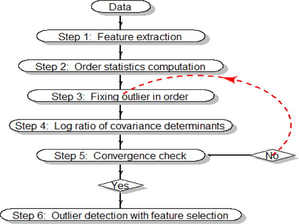
The covariance based outlier detection algorithm, diagrammatically shown in Fig. 1, extends our multivariate Voronoi outlier detection approach [5] through a powerful feature selection procedure. Each of these steps is now discussed in more detail.

Figure 1.

Covariance based outlier detection with feature selection.

Step 1 — Feature extraction

Features have the capacity to be more informative than the data itself [6]. Without loss of generality, suppose the original data are multivariate time series with n observations and p columns of variables. Feature vectors of length n can be extracted from the multivariate time series data. The 13 example feature vectors in this study are overviewed in Table 1; but there is no limit to the number and type of features one could use.

TABLE I.

Feature Labels and description

	Feature Description
F1	Multivariate Least Trimmed Squares
F2	Reweighted Multivariate Least Trimmed Squares
F3	Model based determinant of covariance matrix
F4	Model based trace of covariance matrix (i.e. sum of variances)
F5	Model based determinant of correlation matrix
F6	Model based product of variances
F7	Model free determinant of covariance matrix
F8	Model free trace of covariance matrix (i.e. sum of variances)
F9	Model free determinant of correlation matrix
F10	Model free product of variances
F11	Sum of absolute value of time series observations
F12	Model based sum of squared residuals
F13	Literature based Multivariate Least Trimmed Squares [7]

Features 3, 4, 5 and 6 require first fitting a parametric autoregressive (AR) time series model whereas Features 7, 8, 9 and 10 are the model free analogues which operate just on the raw data. Features 11 and 12 are closely related to the time series data. Features 1, 2 and 13 are binary indicator vectors derived based on the Multivariate Least Trimmed Squares estimator [7, 8], an important classical statistical method for outlier detection.

All features except F13 implement a leave one out approach. For a given feature, its statistic is first computed on all data except the first observation. The first observation is added back, the second observation is removed and the statistic is computed again. This process is repeated for all observations, yielding a n × 1 vector for each feature. If an observation is influential (i.e. outlier), removing it will lead to a less extreme feature value than leaving the observation in the data. At each time point, the features are calculated based on the following descriptions.

F3 and F7 are the inverse determinant of the covariance, 1/det(S), where S is the covariance matrix at the current time point. F3 is based on the covariance matrix after fitting an autoregressive (AR) time series model, and F7 uses the raw data covariance only.

F4 and F8 are the inverse of the trace of the covariance, 1/tr(S). F4 is calculated after fitting an AR model, and F8 is based on the raw data.

F5 and F9 derive from the correlation matrix, R, which is a scaled version of the covariance matrix at the current time point. F5 requires first fitting an autoregressive model, and F9 is from raw data: 1/det(R).

F6 and F10 are the inverse product of the variance terms,

$$1/\mathrm{\Pi }({\sigma }_i)i=1,\dots ,p$$ (1)

where σ_t is the variance at the current time point for variable i. F6 is AR model based and F10 is the corresponding model free version.

F11 sums across the absolute value of the time series for each observation:

$$\sum (y_i),i=1,\dots ,p$$ (2)

where y_i represents the original time series observation at the current time point for variable i.

F12 fits an AR model and then sums across the squared residuals for each observation:

$$\sum {(r_i)}^2,i=1,\dots ,p$$ (3)

where r_i is the residual after fitting the AR model.

F13 is the MLTS, which is a robust statistical method for fitting an AR model while handling outliers [7, 8]. It finds h observations (out of n) whose covariance matrix has the lowest determinant. At each iteration, a subset of randomly selected observations of size h is taken and the mean T₁ and the covariance matrix S₁ are computed to determine the distance d for each observation:

$$d(j)={({({\mathit{y}}_{j^{-}}{\mathit{T}}_{\mathit{1}})}^t(1/{\mathit{S}}_{\mathit{1}})({\mathit{y}}_{j^{-}}{\mathit{T}}_{\mathit{1}}))}^{\mathit{1}/\mathit{2}},j=1,\dots ,n,$$ (4)

where superscript t denotes matrix transpose. The distances from (4) are sorted from smallest to largest, and the h smallest are retained as h₂. From h₂ a new mean T₂ and variance/covariance matrix S₂ are computed. The relationship expressed in (5) now holds:

$$\det ({\mathit{S}}_{\mathit{2}})\le \det ({\mathit{S}}_{\mathit{1}}).$$ (5)

These steps are repeated until the smallest overall determinant is obtained and this subset is the outlier free set of F13 with indicator value 0. The observations outside this subset are assigned with F13 indicator value 1.

F1 is identical to F13 except that F1 implements the leave one out approach. F2 is identical to F1, except the values obtained in equation (5) are compared to a chi-square distribution (χ²) distribution with q degrees of freedom for a given p-value, where q is defined as pk +1, and k is the estimated autoregressive model order. This chi-square distribution represents a particular assumption about the error in the data [8]. If the calculated distance in equation (4) is less than the corresponding chi-square critical value, the observation at the current time point is retained as outlier free for feature F2 with indicator value 0. Otherwise, F2 with indicator value 1 is assigned.

Step 2 — Order statistics computation

For each feature vector, order statistics are computed. The sorting operation happens on the feature vector, so the maximum value is listed first and the minimum value is last. The observations corresponding to each feature value are shuffled according to the order statistics of the feature value. Once the order statistics are computed for all feature vectors, the order sorted feature vectors now encode outlier predictions. The largest feature value is most likely to be an outlier. Two features can theoretically have different statistical or mathematical underpinnings but could still make identical predictions. In this case, those features are redundant. Steps 3, 4 and 5 proceed iteratively.

Step 3 — Fixing outlier in order

For a given feature vector, the observation under consideration that is predicted to be an outlier is corrected by interpolating with the adjacent observations in the un-sorted data.

Step 4 — Log ratio of covariance determinants

After the predicted outlier has been corrected through interpolation, the determinant of the covariance matrix is computed. A determinant can be geometrically interpreted as a volume, where a larger relative volume reflects data with more extreme values. A log of the ratio between the current determinant and the determinant from the 1-step back interpolation is computed. If this ratio is unchanging, this suggests no further outliers are present. But as long as the ratio is decreasing this suggests the feature continues to identify outliers.

Step 5 — Convergence check

After each interpolation, and computing the log ratio of the covariance determinant described in Step 4, convergence is checked. If the log ratio of the determinants approaches 0 (the theoretical minimum), or some small value like .05 which is more reasonable in practice, the feature has identified all of its predicted outliers. If the log ratio of the determinants is not 0 (or close to it), then the algorithm repeats steps 3, 4 and 5. The number of iterations to reach convergence (excluding the current iteration) determines the number of outliers predicted by that feature.

Step 6 — Outlier detection with feature selection

Plotting the convergence (i.e. the determinant of the covariance after fixing the candidate outlier) for all features over the iterations will yield different patterns. Good features will have log ratios that drop quickly (because they are accurately predicting and correcting outlying observations), have a sharp bend and then level off at a constant value near 0. In fact, the iteration at which the bend occurs is the number of outliers detected by a given feature. Poor features take more iterations to converge, or will not obtain near 0 log ratios.

III. Experiments and Results

25 multivariate time series data sets of 5 variables and 100 observations were generated for each of the 15 outlier conditions. The 15 conditions were all combinations of 5, 10 or 15 outliers with magnitudes of 1, 2, 3, 4 or 5. Each multivariate time series was simulated from an AR(2) process with standard normal Gaussian noise. For each outlier condition and for each feature, a receiver operating characteristic (ROC) curve was constructed by using convergence thresholds ranging from 0 to 1, with a step size of .01.

Table II presents a summary of these ROC results. The entries of Table II were computed by taking the maximum and average of the ratio of the true positive rate (TPR) divided by the false positive rate (FPR). Larger values are better. Within a condition, we see variability across features. For instance, F2 has a max of 26 whereas F1 has a max of 1097. We also see variability within a feature, as we consider 5, 10 or 15 outliers. Generally speaking, good features will have large values within a column, relative to other columns and demonstrate consistency across outlier conditions. Magnitudes differ within a column because different outlier conditions have differing levels of detection difficulty, for example, it is much easier to identify 10 outliers with magnitude 5 as compared to 5 outliers of magnitude 1.

TABLE II.

Maximum and Average Ratio of TPR over FPR for all 13 Features

		F1	F2	F3	F4	F5	F6	F7	F8	F9	F10	F11	F12	F13
5 outliers all magnitudes	Max.	1097	26	1079	1023	107	1042	1116	911	233	930	251	967	949
	Ave.	118	5	108	87	24	86	123	119	39	122	53	89	125
10 outliers all magnitudes	Max.	1804	40	695	810	246	818	880	792	414	810	128	739	713
	Ave.	93	5	48	67	54	67	71	49	75	52	36	50	42
15 outliers all magnitudes	Max.	1129	12	592	575	365	299	288	631	387	620	80	625	598
	Ave.	44	3	38	35	30	27	22	20	29	30	20	20	27

Fig. 2 plots the log of the results in Table II, but adds two lines for the overall average across all 15 outlier conditions for the maximum and average. The lines representing the maximum always have larger values than the lines representing the average; but generally the max and average have a similar pattern for all feature vectors. Features with larger values (whether the maximum or average) are better at detecting outliers - like F1 and F3 - whereas features with smaller values - like F2 and F11 - do a poor job of identifying outliers. This figure also shows that it is more difficult for any feature - good or poor - to identify more outliers. We see that higher maximum or average values are obtained for 5 outliers and smaller values for the 15 outlier condition.

Figure 2.

Maximum and average values for 3 outlier conditions (5, 10 or 15 outliers) and all outlier conditions (thick line). x-axis is the labels of features vectors. y-axis is the log of the ratio of the TPR over the FPR. (This figure plots the log of the values in Table II.)

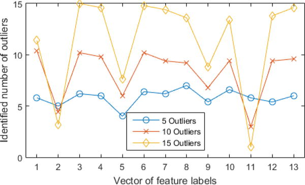
Fig. 3 shows the number of outliers identified by each feature vector for 5, 10 and 15 outlier conditions. If a feature predicted 5 outliers, then it should have its plot symbol at 5. For F4 and F6, we see that it accurately predicts 5, 10 or 15 outliers for each of those conditions. But F2 fails because it predicts 5 outliers (or fewer) for all 3 outlier conditions.

Figure 3.

Number of outliers identified by each feature vector. x-axis is the label of feature vectors and y-axis is the identified number of outliers.

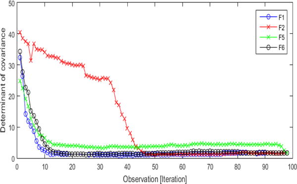
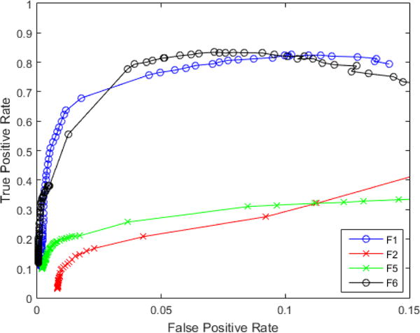
Fig. 4 shows the covariance of the determinant at each iteration for F1, F2, F5 and F6. Fig. 5 is the accompanying ROC plot for those same features. These features showcase the range of variability in feature vectors — 2 good and 2 poor. In Fig. 4, good features like F1 and F6 reach a bend quickly and level off close to 1 because this is the determinant of the covariance for an autoregressive model with Gaussian normal noise. Poor features, like F2 and F5 have a different pattern. F2 does not drop as quickly and only reaches the floor about halfway through the dataset, which would indicate that feature predicted half the observations as outliers. F5 seems to start as a good feature because it drops off fairly quickly; but notice that it levels off at a higher point on the y-axis than F1 and F6, which implies that it may have not identified all the outlier points. It is the combination of the iteration number of where the bend occurs and the curves proximity to 1 once it levels off that determine the number of outliers and if convergence was reached.

Figure 4.

Convergence plot for F1, F2, F5 and F6. x-axis is observation (or iteration) and the y-axis is the determinant of the covariance matrix.

Figure 5.

ROC plot for F1, F2, F5 and F6. x-axis is FPR and y-axis is TPR.

The corresponding ROC curves in Fig. 5 show the good features (F1 and F6) with high TPRs whereas the poor features (F2 and F5) have low TPRs when they are compared at the same FPRs. F6 performs well most likely due to the leveraged covariance information in the data. F5 is a standardized version of the covariance matrix. For outlier detection, variance may be critical. Suppressing it makes the feature unlikely or unable to predict outliers effectively. The pattern of results in Fig. 5 demonstrates that our covariace based mehtod can simultaneously selct a good set of candidate featuure vectors and, from that candidate or effective set, accurately predict outliers.

IV. Conclusions

Many outlier detection algorithms are effective insofar as one has prior knowledge about their data and the outliers. But for some applications, this assumption is not possible. Our covariance based outlier detection algorithm presented here is effective and powerful because it allows a user to specify any number and type of features from the data and the algorithm will determine which features are best and, from that set of good features, correctly identify the number of outliers in the data. Future work could include developing the corresponding counterpart of the method in frequency domain, and testing out the approach on real application data, etc.

References

- 1.Bender E. Big data in biomedicine: 4 big questions. Nature. 2015;527:S19. doi: 10.1038/527S19a. [DOI] [PubMed] [Google Scholar]
- 2.Wang MY, Zwilling CE. Multivariate computing and robust estimating for outlier and novelty in data and imaging sciences. Advances in Bioengineering. 2015:317–336. [Google Scholar]
- 3.Barnett V, Lewis T. Outliers in statistical data. 3rd. Chichester: Wiley; 1994. [Google Scholar]
- 4.Hubert M, Debruyne M. Minimum covariance determinant. Wiley Interdisciplinary Reviews: Computational Statistics. 2010;2:36–43. [Google Scholar]
- 5.Zwilling CE, Wang MY. Multivariate voronoi outlier detection for time series. IEEE Healthcare Innovation and Point-of-Care Technologies Conference. 2014:300–303. doi: 10.1109/HIC.2014.7038934. [DOI] [PMC free article] [PubMed] [Google Scholar]
- 6.Liu H, Motoda H. Feature Selection for Knowledge Discovery and Data Mining. Springer Science & Business Media; 2013. [Google Scholar]
- 7.Agullo J, Croux C, Aelst SV. The multivariate least-trimmed squares estimator. Journal of Multivariate Analysis. 2008;99:311–338. [Google Scholar]
- 8.Croux C, Joossens K. Robust estimation of the vector autoregressive model by a least trimmed squares procedure. Proceedings in Computational Statistics. 2008:489–501. [Google Scholar]