

We show how coastal planners can use sea-level gradient fingerprints to inform mitigation efforts for their local port city.
Abstract
There is a general consensus among Earth scientists that melting of land ice greatly contributes to sea-level rise (SLR) and that future warming will exacerbate the risks posed to human civilization. As land ice is lost to the oceans, both the Earth’s gravitational and rotational potentials are perturbed, resulting in strong spatial patterns in SLR, termed sea-level fingerprints. We lack robust forecasting models for future ice changes, which diminishes our ability to use these fingerprints to accurately predict local sea-level (LSL) changes. We exploit an advanced mathematical property of adjoint systems and determine the exact gradient of sea-level fingerprints with respect to local variations in the ice thickness of all of the world’s ice drainage systems. By exhaustively mapping these fingerprint gradients, we form a new diagnosis tool, henceforth referred to as gradient fingerprint mapping (GFM), that readily allows for improved assessments of future coastal inundation or emergence. We demonstrate that for Antarctica and Greenland, changes in the predictions of inundation at major port cities depend on the location of the drainage system. For example, in London, GFM shows LSL that is significantly affected by changes on the western part of the Greenland Ice Sheet (GrIS), whereas in New York, LSL change predictions are greatly sensitive to changes in the northeastern portions of the GrIS. We apply GFM to 293 major port cities to allow coastal planners to readily calculate LSL change as more reliable predictions of cryospheric mass changes become available.
INTRODUCTION
Ice sheets, glaciers, and ice caps have contributed significant sea-level rise (SLR) throughout the 20th century (1, 2), with a noticeable acceleration in the early 21st century (2). The recent increases are likely attributable to changes in the surface melting of the Greenland Ice Sheet (GrIS) as well as the acceleration of its outlet glaciers (3), the West Antarctic Ice Sheet (WAIS) (4) and the Antarctic Peninsula Ice Sheet (APIS). These contributions are likely to increase in the future (5–8). Given the widely disparate spatial distribution of on-land ice thickness changes, the pattern of sea level will be highly sensitive to the detailed mass loss geometry for each cryosphere component (9). When land ice is lost to the oceans, SLR exhibits a strong pattern [termed a sea-level fingerprint (10)] following the ice-induced perturbations in the Earth’s gravitational and rotational potentials and the associated solid Earth deformation (11–13). Sea level here is defined as the change in ocean water depth rather than the change in radial position of the sea surface.
For example, scenarios of submarine ice sheet collapse of WAIS (10, 14) predict a sea-level inundation of an order 25% larger than the globally averaged rise for both the western and eastern shorelines of the continental United States. However, there is great uncertainty in how the demise of the on-land cryosphere will occur during projected planet-wide warming (15), and this fact hobbles the ability of policy makers and coastal planners to accurately quantify local sea-level (LSL) projections upon which sound mitigation and remediation strategies are built.
Building on sea-level fingerprints, estimates of how much coastal LSL can be expected and its sensitivity to ice thickness change have been evaluated in several studies (16–19). However, the resolution in these analyses was coarse, owing mainly to the sparsity of information about the ice thickness change distribution itself. In the far field, the sensitivity of fingerprints to ice loading is minimal. However, in the near field, or for areas with strong rotational feedback and/or vertical motion of the elastic crust, this sensitivity is arguably poorly understood. For these cases, there is a great impetus to leverage the full range of advanced mathematical capabilities to optimally combine observational data, forward model projections, and uncertainty quantification to help coastal planners better constrain the range of LSL projections. Here, we exploit the powerful adjoint method often applied in seismology, meteorology, and oceanography (20, 21), combined with automatic differentiation of the Ice Sheet System Model (ISSM) (22, 23), to complete a comprehensive computation of the Jacobian of the sea-level fingerprints: the derivative dS/dH of sea level, S, with respect to changes in ice thickness, H, in glaciated areas around the entire world. Our focus is not on specific fingerprints from polar ice sheets or specific glaciers but rather on a comprehensive computation of dS/dH for any glaciated load. Our design is to use dS/dH at specific locations to accurately map observations [be it from space and airborne altimetry (24) or from space gravimetry (25)], or projections (15) of global ice thickness change, into actionable signals of LSL change that are both highly resolved spatially and fully consistent with the physics of sea-level evolution. Our goal is not to improve knowledge of how the on-land ice thickness will change in time but rather to improve our understanding of the connection between global cryospheric changes and LSL at major port cities around the globe.
APPROACH
Our approach builds on the conventional method of mapping ice thickness changes into sea-level fingerprints using the following equation
| (1) |
where “local” refers to the location of the port city of interest, “ice” is the domain over which glaciated changes are occurring, (θ,λ) represents the geographic coordinates on Earth’s surface, t is the time, dA is an elementary integration area on the globe, and ΔSlocal(t) is the quantity coastal planners wish to assess, given a set of observations or projections about variations in ice thickness, ΔH, around the world. Here, dS/dH|local is the value of the Jacobian at a specific location, also referred to as the gradient of the sea-level fingerprint. For convenience, we refer to the approach of computing ΔSlocal(t) through gradient fingerprints dS/dH as gradient fingerprint mapping (GFM), a method that has the advantage of applying to a wide range of loading scenarios (26). Furthermore, it provides information about the exact departure from global mean sea level (GMSL) at a specific location. By convolving gradient fingerprints and ice thickness changes over the entire planet, the departure from the GMSL is fully recovered. We note that an additional component δSlocal(t) is required in Eq. 1 to account for the dynamic/thermosteric ocean component and local vertical land motion due to various anelastic and creep responses of the earth that can be related to coastal subsidence/emergence. We also note that only secular changes to LSL are considered here (not including short time scale processes such as waves, storms, or tides). δSlocal can be evaluated by model simulation and coastal observational systems. Although δSlocal is important, the most severe risk of future SLR on century or longer time scales arises from the potential demise of ice sheets (6, 7, 14, 27). We also note that GFM is applicable to any location on the globe, where other types of mass change might occur (for example, through hydrological fluxes or snow cover changes), although our focus here is on glaciated areas.
To compute the Jacobian, dS/dH, we rely on the classic equations for the static response of the ocean surface and potential field on a static, compressible, elastic, self-gravitating Earth (11). With the inclusion of change in the rotational potential (12, 13), these equations relate sea level to perturbations in the Earth’s gravitational and rotational fields induced by local mass changes (cf. Materials and Methods), combined with the elastic adjustment of the earth (here, the viscous component of Earth deformation is not included). Henceforth, these equations are referred to as the spherically symmetric rotating Earth (SRE) equations. In these equations, loading and deformational responses may come from variations in ice thickness, hydrological fluxes, or any process affecting the distribution of mass (28). However, to achieve high-resolution estimates of the derivative dS/dH, a prohibitive number of SRE runs are required to carry out forward differencing. In addition, forward differencing only achieves an approximation of the derivative, dependent on the forward step size. Here, we use a far more comprehensive approach of automatic differentiation and the adjoint method (22, 23) for SRE, which computes the machine precision derivative dS/dH for any glaciated location in the world (cf. Materials and Methods).
RESULTS AND DISCUSSION
An example is shown in Fig. 1A for New York, where the gradient has been computed for all glaciated areas of the world. The approach is highly precise and can be easily scaled when combined with the anisotropic meshing approach to solving the SRE equations (29), which allows for mesh refinement near the city of interest as well as near the glaciated areas that might also be of relevance to coastal planning. In addition, the approach relies on the highly parallelized infrastructure of ISSM (30), which allows dS/dH to be computed at spatial scales that can capture complex coastline configurations.
Fig. 1. Sensitivity of SLR to worldwide variations in ice thickness.
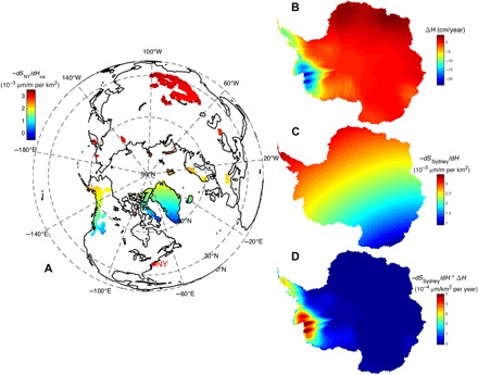
(A) Gradient −dSNY/dH (in 10−3 μm/m per km2) of sea level in New York (SNY) with respect to ice thickness (H) changes in glaciated areas. The gradient units reflect a measure of SLR change (in μm) per unit of ice thickness change (in m) per area unit of ice (in km2), which is equivalent to SLR change (in mm) per unit change in ice mass (in GT). Signs rendered for dS/dH result in positive sensitivities of SLR to negative thickness changes (that is, shrinking ice sheets and glaciers resulting in positive GMSL rise). (B) GRACE-inferred ice thickness change (in cm/year) for Antarctica during January 2003–December 2015, demonstrating strong spatial variability. (C) Gradient −dSSydney/dH (in μm/m per km2) of sea level in Sydney (SSydney) with respect to ice thickness (H) changes in Antarctica. (D) LSL contribution −dSSydney/dH*ΔH (in μm/km2 per year) for each km2 area of Antarctica to LSL in Sydney. The sum of this quantity over the entire ice sheet quantifies the contribution of the entire AIS to LSL in Sydney. Coastlines are plotted in black.
In contrast to a specific SRE forward run, GFM can be used for coastal planning at a specific location. For example, when applied to the port city of Sydney, Australia, Antarctic mass trends mapped by Gravity Recovery and Climate Experiment (GRACE) from January 2003 to December 2015 (Fig. 1B) are certainly important for the prediction of LSL change. However, additional information is revealed in the gradient results shown in Fig. 1C, for the map shows that LSL changes at the port are very strongly influenced by ice changes that occur along the north-northeast and north-northwest coasts, an area that includes the APIS. When both maps are combined (Fig. 1D), GRACE observations and gradient fingerprints reveal that the port city of Sydney must be concerned not only by the ice loss in the Amundsen Sea Sector (the deepest red region in Fig. 1D) but also by the rapid demise of ice in the APIS and its recent loss of buttressing forces caused by a series of precipitous ice shelf collapses (31). The relative importance of these two regions (Amundsen Sea Sector versus APIS) may be quantified by a ratio of approximately 5 to 3 (per km2 of ice) during the GRACE period.
To demonstrate scalability, we apply similar computations to 293 of the world ports and to the locations of long-recording, high-quality tide gauge stations (32). Figure 2 shows a subset of port cities along the Canadian and U.S. coastlines with focus on the values of the gradient fingerprints for Greenland, demonstrating the important impact of the proximity to the GrIS for cities such as Halifax or New York. A clear rotation of the gradients moving counterclockwise along the U.S. coastline, corresponding to the magnitude lines of the underlying sea-level fingerprint, is also shown. Especially useful for policy makers are maps that are normalized by the GMSL gradient values, which enable a quick comparison to what the gradient fingerprint would be in a scenario where LSL is identical to GMSL everywhere in the world. The reference state for the normalizing GMSL gradient is computed using the so-called bathtub model, where sea level is evenly distributed over the entire oceans as though Earth is a nongravitating, nonrotating, rigid planet. This normalization factor is therefore constant for any city and any location in the world. Figure 3 shows normalized maps for Europe, illuminating the fact that cities lying along the Mediterranean shoreline, far from Greenland, have gradient fingerprints that are almost fully consistent with the GMSL gradient (ratio ≈ 100%). Deviations from the GMSL gradient grow larger the closer the city is to Greenland, consistent with a decrease in sea level (due to gravitational effects), with Brest, London, Oslo, and Tromso having substantial departures from the GMSL gradient. We remark that the long-wavelength features of the fingerprints may be dominated by the rotational feedback, a feature also noted in previous analyses (10, 14, 26, 28). This is best reflected in the normalized gradient fingerprint, for example, along the African coastlines (fig. S14), where significantly different patterns can be detected for Dar Es Salaam and Luanda. Despite the fact that both cities are essentially equidistant from Antarctica and Greenland, Luanda is closer to the South Atlantic, where rotational feedbacks associated with Antarctic and Greenland mass changes appear to be important.
Fig. 2. Sensitivity of SLR along U.S./Canadian coastlines to GrIS thickness variations.
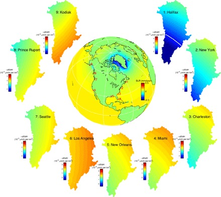
Gradient −dS/dH (in 10−3 μm/m per km2) at U.S. and Canadian coastal cities. Maps 1 to 9 correspond, respectively, to gradients computed for each of the named ports numbered clockwise from Halifax. −dS/dH is computed using the ISSM-AD (23) gradient solver. The forward SLR run used to support the derivation of –dS/dH is shown in the center Earth map (in mm/year). It is computed using the ISSM-SESAW (29) solver with model inputs (ice thickness change) inferred from GRACE for the period 2003–2016. This forward model therefore captures the response to thickness changes in all of the main glaciated areas of the world (including, among others, Alaskan and Canadian Arctic Glaciers, Himalayan Glaciers, Patagonia Glaciers, and the Greenland and Antarctica Ice Sheets) (28), hence representing a truly global “ice” fingerprint.
Fig. 3. GMSL ratios for select coastline cities across Europe applied to GrIS.
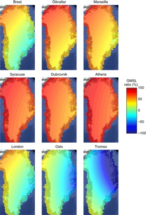
GMSL ratios (in %) for coastal cities across Europe (from −100 to 100%). The ratios are defined as gradients of local SLR with respect to changes in ice thickness, −dS/dH, normalized by the equivalent GMSL gradient –dSGMSL/dH, where SGMSL is the GMSL signal induced by an equivalent change in ice thickness. These ratios measure the departure from GMSL contributed by local ice thickness changes in Greenland. They can be used to multiply against observed/predicted ice thickness changes to quantify any non-GMSL effects at any coastal city of the world.
Because GFM is only dependent on the surface load, and not time variations (if we assume a purely elastic Earth), it can be applied to evaluate the future ensembles of scientific predictions anticipated for Greenland or other glaciated areas. To illustrate this application, we use the Sea-level Response to Ice Sheet Evolution (SeaRISE) benchmark experiments (15), which were designed to better understand the sensitivity of ice-flow models to plausible boundary conditions and initializations. We apply GFM to a subset of two SeaRISE experiments representative of the wide spread in the simulations for GrIS (cf. Materials and Methods). The projection period is 200 years, and for demonstration purposes, we assume that this period is short enough for the elastic response field of our SRE solver (29) to remain valid. The hypothesis is not strictly true when viscous behavior becomes significant and the computation of the gradient is then complicated by load history, lithospheric thickness, and mantle viscosity profile. The effects might be quite complex and spatially variable, particularly in coastal regions where the impact of ocean loading depends on the geometry of the shoreline and possible three-dimensional viscosity structure. In particular, sea-level drop will be exacerbated in the near field and LSL rise in the intermediate and far fields (33), away from the ice basin losing mass. Here, using the two SeaRISE ice-flow runs, we retrieve projected ice thickness changes after 200 years and convert them (using Eq. 1) into an equivalent SLR contribution from each local area in Greenland and show the results for New York and London and for any geographical location that experiences only the GMSL variation (Fig. 4). The maps in Fig. 4 reveal strong spatial variations in predictions of local and total SLR contribution from the GrIS, relative to the GMSL contribution. For New York, the gradient (see Fig. 2) decreases in a northeast to southwest direction, which results in a strong contribution to LSL in New York that is mainly caused by ice loss through the Petermann Glacier, Humboldt Glacier, and North-East Greenland Ice Stream. Because of a strong signal in the predicted ice thickness decrease in Jakobshavn Glacier, this glacier still remains a contributor, but to a lesser degree. For London, the gradient (see Fig. 3) decreases from a northwest to southeast direction, resulting in a strong contribution from the Petermann Glacier, Humboldt Glacier, and Ostenfeld Glacier and a somewhat lesser contribution from the North-East Greenland Ice Stream. For both cities, the entire area south of 77°N contributes very modestly to the LSL signal. A model average for both runs shows a New York SLR contribution owing to GrIS to be 50% of the projected GMSL and 17.7% for London. This demonstrates the importance of refining both the magnitude and spatial distribution of projections of ice thickness change, and shows an example of application of GFM to understand which basin, in particular, is responsible for LSL at a specific location.
Fig. 4. Projected contribution of GrIS to SLR in New York and London based on the SeaRISE experiments.
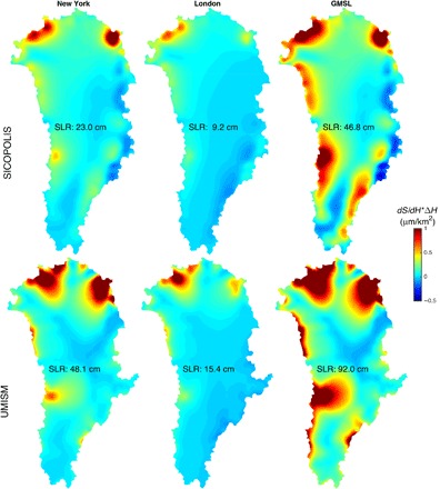
Two hundred–year projection of the contribution (in μm/km2) of local areas in Greenland to SLR in New York (first column), London (second column), and any geographical location that experiences only the GMSL variation (third column) using two models of ice thickness change from the SeaRISE (15) experiments: Simulation Code for Polythermal Ice Sheets (SICOPOLIS) and University of Maine Ice Sheet Model (UMISM). The units reflect a measure of SLR change (in μm) per area unit (in km2) of the GrIS. It is equal to the gradient fingerprint multiplied by the GrIS thickness change, or dS/dH|local*ΔH, where dS/dH|local is the gradient fingerprint for the local port city and ΔH is the projected ice thickness change for the GrIS. This localized contribution can be summed up over the entire GrIS to compute SLR for London, for example, . For reference, we provide total SLR computed for London, New York, and the GMSL scenario. Note that in these two SeaRISE GrIS projections, both London and New York have LSL changes that are reduced over the GMSL rise that will affect far-field cities.
In Table 1 (and associated fig. S1), we extend this approach to describe a roadmap for applying GFM that will enhance coastal planning at the local level. For a specific city, GFM provides dS/dH, the gradient of LSL with respect to ice thickness changes in the world (figs. S2 to S20). This gradient then needs to be combined with an estimate of ice thickness change, ΔH. Here, we rely on an average of the two SeaRISE runs considered in Fig. 4. Observations such as GRACE-derived mass changes extrapolated into the future can also be used, as can any estimate from systematic and robust studies, even ones that are not global. By using Eq. 1, given that dS/dH is computed at high spatial resolution, one can quantify the contribution of any area to LSL at the port city considered. For example, Table 1 presents the contribution of four large basins of Greenland—Petermann Glacier, Helheim Glacier, North-East Greenland Ice Stream, and Jakobshavn Glacier—to LSL in 30 cities across all continents. The computation is virtually instantaneous (provided that the gradients are precomputed) and provides insights into how much LSL each city will experience compared to GMSL and which basins each city should be concerned with. The analysis was carried out at a resolution compatible with each catchment basin for each glacier. However, it could be carried out at a much more refined resolution. This is helpful for Greenland where the number of glaciers is significant. The degree of refinement will depend on the priorities of each coastal planner. In particular, for glaciated areas far from the port city, a coarse resolution would be fine, with increased granularity in the analysis for glaciated areas close to the city itself. In addition, GFM accommodates the analyses of the associated uncertainties in the ice thickness changes, which can be transferred into an equivalent LSL uncertainty range using Eq. 1. This allows coastal planners to instantly derive uncertainty in their local LSL projection by ascribing different scenarios of ice thickness change, according to existing observations, extrapolations thereof, newly released state-of-the-art estimates of projected ice thickness changes, or specific publications focusing on particular basins.
Table 1. Contribution of Greenland catchment basins to LSL.
GFM-derived contribution of five catchment basins (Petermann Glacier, Helheim Glacier, North-East Greenland Ice Stream, and Jakobshavn Glacier, all delimited in fig. S1) to LSL in 30 cities around the world based on an average of two SeaRISE model runs (see Materials and Methods) over a 200-year time period. For each basin, the projected GMSL value is provided for reference. For each city, a value of LSL is provided in cm, along with a ratio to GMSL in %.
| City | Petermann Glacier: 8.22 cm | Helheim Glacier: 1.4 cm | North-East Greenland Ice Stream: 10.6 cm | Jakobshavn Glacier: 4.41 cm |
| New York | 5.1 cm (62%) | 0.497 cm (36%) | 7.2 cm (68%) | 1.54 cm (35%) |
| Miami | 7.51 cm (91%) | 1.09 cm (78%) | 10.1 cm (95%) | 3.41 cm (77%) |
| Los Angeles | 7.44 cm (91%) | 1.35 cm (96%) | 10.6 cm (100%) | 4.04 cm (92%) |
| Seattle | 5.42 cm (66%) | 1.13 cm (81%) | 8.67 cm (82%) | 3.23 cm (73%) |
| Rio | 10.1 cm (123%) | 1.83 cm (131%) | 13.2 cm (124%) | 5.69 cm (129%) |
| Ushuaia | 10.7 cm (130%) | 1.94 cm (139%) | 13.7 cm (129%) | 6.07 cm (138%) |
| Lima | 9.57 cm (116%) | 1.66 cm (119%) | 12.3 cm (116%) | 5.2 cm (118%) |
| Panama | 8.88 cm (108%) | 1.44 cm (103%) | 11.6 cm (109%) | 4.52 cm (102%) |
| London | 3.38 cm (41%) | −0.174 cm (−12%) | 1.7 cm (16%) | 0.257 cm (6%) |
| Oslo | 1.38 cm (17%) | −0.305 cm (−22%) | −2.24 cm (−21%) | −0.276 cm (−6%) |
| Athens | 6.78 cm (83%) | 0.925 cm (66%) | 7.36 cm (69% | 3.18 cm (72%) |
| Casablanca | 6.51 cm (79%) | 0.647 cm (46%) | 7.3 cm (69%) | 2.45 cm (55%) |
| Luanda | 9.14 cm (111%) | 1.58 cm (113%) | 11.9 cm (112%) | 4.95 cm (112%) |
| Durban | 9.77 cm (119%) | 1.76 cm (126%) | 13.1 cm (123%) | 5.41 cm (123%) |
| Djibouti | 8.55 cm (104%) | 1.42 cm (102%) | 10.7 cm (100%) | 4.52 cm (103%) |
| Alexandria | 7.42 cm (90%) | 1.11 cm (79%) | 8.51 cm (80%) | 3.67 cm (83%) |
| Karachi | 8.56 cm (104%) | 1.48 cm (105%) | 10.5 cm (99%) | 4.69 cm (106%) |
| Colombo | 9.63 cm (117%) | 1.66 cm (119%) | 12.3 cm (116%) | 5.22 cm (118%) |
| Jakarta | 9.69 cm (118%) | 1.64 cm (118%) | 12.5 cm (118%) | 5.16 cm (117%) |
| Brunei | 9.75 cm (119%) | 1.7 cm (122%) | 12.6 cm (118%) | 5.32 cm (121%) |
| Sydney | 8.96 cm (109%) | 1.39 cm (99%) | 11.3 cm (106%) | 4.43 cm (100%) |
| Perth | 8.9 cm (108%) | 1.42 cm (101%) | 11.5 cm (109%) | 4.47 cm (101%) |
| Hong Kong | 9.64 cm (117%) | 1.76 cm (126%) | 12.4 cm (116%) | 5.5 cm (125%) |
| Tokyo | 9.84 cm (120%) | 1.91 cm (136%) | 12.9 cm (122%) | 5.89 cm (133%) |
| Okhotsk | 6.86 cm (83%) | 1.61 cm (115%) | 9.43 cm (89%) | 4.84 cm (110%) |
| Karatayka | 1.71 cm (21%) | 0.638 cm (46%) | −0.398 cm (−4%) | 2.02 cm (46%) |
| Nordvik | 0.819 cm (10%) | −0.621 cm (−44%) | −3.34 cm (−31%) | −1.04 cm (−24%) |
| Reykjavik | −4.85 cm (−59%) | −5.23 cm (−373%) | −12.8 cm (−121%) | −10.2 cm (−231%) |
| Ellesmere | −94.7 cm (−1153%) | −1.2 cm (−86%) | −28.5 cm (−268%) | −6.01 cm (−136%) |
| Barrow | 0.31 cm (4%) | 0.95 cm (68%) | 3.57 cm (34%) | 2.48 cm (56%) |
CONCLUSIONS
Using atmosphere-ocean general circulation models, several recent studies examine the uncertainties in future LSL caused by ocean circulation changes (34, 35). In New York, for example, for an ocean circulation–driven GMSL prediction of 22 to 40 cm, the spread of LSL predictions is [−4, 38] cm at about 2100 (35). However, the amplitude of the predicted GMSL contribution from the cryospheric changes at 2100 is considerably larger, with, for example, Antarctica already projected to contribute potentially more than 1-m GMSL rise at 2100 (6). Although these predicted contributions remain highly uncertain, they imply that the practical risks assessed for future LSL change should include a strong contribution from changes to the now well-monitored mass in the land cryosphere (36). Application of GFM by planners and decision makers will improve on the existing state of the art by enabling improved high-resolution quantification of the sensitivity of LSL evolution to global cryospheric changes. Because numerically based projection models of polar ice sheets and mountain glaciers continue to improve, GFM will have an impact in the way long-term coastal planning is executed.
MATERIALS AND METHODS
SRE forward run
We relied on the SRE (11, 13) equations to solve for sea-level evolution. Our implementation of the solver is based on ISSM-SESAW (29), which operates efficiently on an unstructured mesh. For the purpose of GFM, the following equations are of relevance. First, we define a global mass-conserving load function L(θ,λ,t)
| (2) |
where H is the change in ice thickness on a (global or regional) land ice mask I, S is the associated change in sea level with ocean mask O, ρI is the ice density, and ρO is the ocean water density. Mass changes in land ice, along with the associated variations in ocean loading, induce perturbations in the Earth’s gravitational and rotational potential fields, causing further redistribution of S, which is both gravitationally and deformationally self-consistent. For an elastically compressible rotating Earth, the gravitationally consistent S is given by
| (3) |
where G is a Green’s function that models the influence of a specific point load on relative sea level evaluated at an arc distance α from the load coordinate position (θ′,λ′), Λ2mi are related to perturbations in rotational potential and associated solid Earth deformation induced by the applied loading, Y2mi are analytic (degree-2, order-m spherical harmonic) functions (i’s represent the cosine and sine terms), and E is a spatial invariant required to conserve the mass. Parameters R, M, and g represent Earth’s radius, mass, and gravitational acceleration, respectively. The operator ⊗ implies the spatial convolution on the surface of Earth. Solving Eq. 3 for S requires a priori knowledge of S itself (cf. Eq. 2), and we therefore solve the system of equations iteratively, as in the study of Farrell and Clark (11). For more details on this approach, including validation against other existing methods relying on spherical harmonics, we refer the reader to ISSM-SESAW (29).
Gradient fingerprint
To compute the gradient fingerprint dS/dH in Eq. 1, we relied on the automatic differentiation module ISSM-AD (23). This module is based on overloaded operators as an approach to computing discrete adjoints for a parallelized model (22, 23) and to evaluating higher-order derivatives of this model within machine precision. Using ISSM-AD (23), one can basically tape the entire suite of operations required to carry out a forward run of the ISSM-SESAW solver. Once this is carried out, the gradient of the model output with respect to any model inputs can be computed using the reverse chain rule on the tape itself (which recorded all the operations and the values of each operator at each step). Although this approach might be used to evaluate the entire Jacobian dS/dH of Eq. 3, memory and disk space requirements are excessive, given our mesh of 87,886 elements and 43,945 vertices that we used here to solve the SRE equations and for a computational platform such as the NASA Ames Pleiades cluster. Therefore, the solution is to compute the value of the Jacobian only at specific locations. For each location, we define dS/dH|local as the gradient of the fingerprint for the chosen location “local.” In Figs. 1 (A and C) and 2 and figs. S2 to S22, this gradient was evaluated across 293 locations corresponding to major port cities in the world and an additional 15 high-quality tide gauge locations (32). H spans the entire world where areas are glaciated, including, among others, the GrIS, AIS, Alaskan, Arctic, Patagonian, and Himalayan glaciers (see Fig. 1A). Note that, here, we restrict ourselves to H as the only independent variable, although the Jacobian could also be computed with respect to other independent variables. This could include, for example, ocean circulation and/or viscous response of the solid earth, among others.
SeaRISE experiments
The SeaRISE experiments provide quantitative projections of Greenland and Antarctica over the next 500 years. A number of ice sheet models were simulated under the representative concentration pathway emission scenario 8.5 (RCP 8.5) and its suitable extension beyond CE 2100. The radiative forcing associated with the emission scenario drives the ice sheet models through surface climatology, basal sliding, and ice shelf melting. In our analysis, we relied on two model runs for the GrIS that were involved in the RCP 8.5 experiment: SICOPOLIS and UMISM. These two runs represent end members of the ensemble of runs carried out for RCP 8.5 that were computed for at least 200 years. Our purpose in using these SeaRISE experiments was to demonstrate the impact of amplitude and spatial structure of ice mass changes on SLR at select coastal cities, using an ensemble representative of the spread in current model projections of the GrIS (see Fig. 4).
Data release
GFM computed gradients for cities and tide gauge locations in Fig. 1 and figs. S2 to S22 are available for direct download in the Jet Propulsion Laboratory (JPL) Virtual Earth System Laboratory (https://vesl.jpl.nasa.gov/research/sea-level/slr-gfm) as well as the NASA Sea-Level Science Team Portal website (https://sealevel.nasa.gov/vesl/web/research/sea-level/slr-gfm/).
Supplementary Material
Acknowledgments
We would like to thank F. Landerer at JPL for his valuable feedback and insights into the study. Funding: This work was performed at the JPL, California Institute of Technology, under a contract with the JPL Research, Technology and Development Program (grant #01STCR R.15.181.047; 2015–2017), the NASA Cryospheric Sciences Program (grant #509496.02.08.06.21; 2014–2016), the NASA Modeling and Analysis Program (grant #281945.02.04.02.63; 2014–2017), the NASA Earth Surface and Interior Focus Area Program (grant #281945.02.47.03.86; 2014–2017), the NASA Sea-Level Change Science Team (grant #281945.02.47.03.33; 2015–2017), and the NASA GRACE Science Team (grant #E.8.1.1; 2016–2017). Author contributions: All authors contributed to the theory. E.L. led the calculations. E.R.I. and S.A. assisted with the interpretation of the results. All authors contributed to the writing of the paper. Competing interests: The authors declare that they have no competing interests. Data and materials availability: All data needed to evaluate the conclusions in the paper are present in the paper and/or the Supplementary Materials. Additional data related to this paper may be requested from the authors.
SUPPLEMENTARY MATERIALS
Supplementary material for this article is available at http://advances.sciencemag.org/cgi/content/full/3/11/e1700537/DC1
fig. S1. Greenland basins used in Table 1.
fig. S2. Sensitivity of SLR along the South American coastline to GrIS thickness variations.
fig. S3. Sensitivity of SLR along the European coastline to GrIS thickness variations.
fig. S4. Sensitivity of SLR along the African coastline to GrIS thickness.
fig. S5. Sensitivity of SLR along the Middle East and South Asian coastlines to GrIS thickness variations.
fig. S6. Sensitivity of SLR along the Southeast Asian coastline to GrIS thickness variations.
fig. S7. Sensitivity of SLR along the Australian coastline to GrIS thickness variations.
fig. S8. Sensitivity of SLR along the East Asian coastline to GrIS thickness variations.
fig. S9. Sensitivity of SLR along the Northeast Asian and the Russian Arctic coastlines to GrIS thickness variations.
fig. S10. Sensitivity of SLR along the Canadian Arctic coastline to GrIS thickness variations.
fig. S11. Sensitivity of SLR along the North American coastline to AIS thickness variations.
fig. S12. Sensitivity of SLR along the South American coastline to AIS thickness variations.
fig. S13. Sensitivity of SLR along the European coastline to AIS thickness variations.
fig. S14. Sensitivity of SLR along the African coastline to AIS thickness variations.
fig. S15. Sensitivity of SLR along the Middle East and Southeast Asian coastlines to AIS thickness variations.
fig. S16. Sensitivity of SLR along the Southeast Asian coastline to AIS thickness variations.
fig. S17. Sensitivity of SLR along the Australian coastline to AIS thickness variations.
fig. S18. Sensitivity of SLR along the East Asian coastline to AIS thickness variations.
fig. S19. Sensitivity of SLR along the Northeast Asian and the Russian Arctic coastlines to AIS thickness variations.
fig. S20. Sensitivity of SLR along the Canadian Arctic coastline to AIS thickness variations.
fig. S21. Sensitivity of SLR for 15 reliable tide gauges around the world to GrIS thickness variations.
fig. S22. Sensitivity of SLR for 15 reliable tide gauges around the world to AIS thickness variations.
REFERENCES AND NOTES
- 1.Meier M. F., Dyurgerov M. B., Rick U. K., O’Neel S., Pfeffer W. T., Anderson R. S., Anderson S. P., Glazovsky A. F., Glaciers dominate eustatic sea-level rise in the 21st century. Science 317, 1064–1067 (2007). [DOI] [PubMed] [Google Scholar]
- 2.Church J. A., White N. J., A 20th century acceleration in global sea-level rise. Geophys. Res. Lett. 33, L01602 (2006). [Google Scholar]
- 3.Rignot E., Kanagaratnam P., Changes in the velocity structure of the Greenland ice sheet. Science 311, 986–990 (2006). [DOI] [PubMed] [Google Scholar]
- 4.Rignot E., Bamber J. L., van den Broeke M. R., Davis C., Li Y., van de Berg W. J., van Meijgaard E., Recent Antarctic ice mass loss from radar interferometry and regional climate modelling. Nat. Geosci. 1, 106–110 (2008). [Google Scholar]
- 5.R. K. Pachauri, M. R. Allen, V. R. Barros, J. Broome, W. Cramer, R. Christ, J. A. Church, L. Clarke, Q. Dahe, P. Dasgupta, N. K. Dubash, O. Edenhofer, I. Elgizouli, C. B. Field, P. Forster, P. Friedlingstein, J. Fuglestvedt, L. Gomez-Echeverri, S. Hallegatte, G. Hegerl, M. Howden, K. Jiang, B. Jimenez Cisneroz, V. Kattsov, H. Lee, K. J. Mach, J. Marotzke, M. D. Mastrandrea, L. Meyer, J. Minx, Y. Mulugetta, K. O’Brien, M. Oppenheimer, J. J. Pereira, R. Pichs-Madruga, G. K. Plattner, H. O. Pörtner, S. B. Power, B. Preston, N. H. Ravindranath, A. Reisinger, K. Riahi, M. Rusticucci, R. Scholes, K. Seyboth, Y. Sokona, R. Stavins, T. F. Stocker, P. Tschakert, D. van Vuuren, J. P. van Ypserle, Climate Change 2014: Synthesis Report Contribution of Working Groups I, II and III to the Fifth Assessment Report of the Intergovernmental Panel on Climate Change (Intergovernmental Panel on Climate Change, 2014), p. 151. [Google Scholar]
- 6.DeConto R. M., Pollard D., Contribution of Antarctica to past and future sea-level rise. Nature 531, 591–597 (2016). [DOI] [PubMed] [Google Scholar]
- 7.Ritz C., Edwards T. L., Durand G., Payne A. J., Peyaud V., Hindmarsh R. C. A., Potential sea-level rise from Antarctic ice-sheet instability constrained by observations. Nature 528, 115–118 (2015). [DOI] [PubMed] [Google Scholar]
- 8.Oppenheimer M., Alley R. B., How high will the seas rise? Science 354, 1375–1377 (2016). [DOI] [PubMed] [Google Scholar]
- 9.Kopp R. E., Mitrovica J. X., Griffies S. M., Yin J., Hay C. C., Stouffer R. J., The impact of Greenland melt on local sea levels: A partially coupled analysis of dynamic and static equilibrium effects in idealized water-hosing experiments. Clim. Change 103, 619–625 (2010). [Google Scholar]
- 10.Mitrovica J. X., Gomez N., Clark P. U., The sea-level fingerprint of West Antarctic collapse. Science 323, 753 (2009). [DOI] [PubMed] [Google Scholar]
- 11.Farrell W. E., Clark J. A., On postglacial sea level. Geophys. J. Int. 46, 647–667 (1976). [Google Scholar]
- 12.Dahlen F. A., The passive influence of the oceans upon the rotation of the Earth. Geophys. J. Int. 46, 363–406 (1976). [Google Scholar]
- 13.Milne G. A., Mitrovica J. X., Postglacial sea-level change on a rotating Earth. Geophys. J. Int. 133, 1–19 (1998). [Google Scholar]
- 14.Bamber J. L., Riva R. E. M., Vermeersen B. L. A., LeBrocq A. M., Reassessment of the potential sea-level rise from a collapse of the West Antarctic Ice Sheet. Science 324, 901–903 (2009). [DOI] [PubMed] [Google Scholar]
- 15.Bindschadler R. A., Nowicki S., Abe-Ouchi A., Aschwanden A., Choi H., Fastook J., Granzow G., Greve R., Gutowski G., Herzfeld U., Jackson C., Johnson J., Khroulev C., Levermann A., Lipscomb W. H., Martin M. A., Morlighem M., Parizek B. R., Pollard D., Price S. F., Ren D., Saito F., Sato T., Seddik H., Seroussi H., Takahashi K., Walker R., Wang W. L., Ice-sheet model sensitivities to environmental forcing and their use in projecting future sea level (the SeaRISE project). J. Glaciol. 59, 195–224 (2013). [Google Scholar]
- 16.J. A. Church, P. U. Clark, A. Cazenave, J. M. Gregory, S. Jevrejeva, A. Levermann, M. A. Merrifield, G. A. Milne, R. S. Nerem, P. D. Nunn, A. J. Payne, W. T. Pfeffer, D. Stammer, A. S. Unnikrishnan, Sea-level change, in Climate Change 2013: The Physical Science Basis. Contribution of Working Group I to the Fifth Assessment Report of the Intergovernmental Panel on Climate Change, T. F. Stocker, D. Qin, G.-K. Plattner, M. Tignor, S.K. Allen, J. Boschung, A. Nauels, Y. Xia, V. Bex, P. M. Midgley, Eds. (Cambridge Univ. Press, 2013). [Google Scholar]
- 17.Church J. A., Gregory J. M., White N. J., Platten S. M., Mitrovica J. X., Understanding and projecting sea-level change. Oceanography 24, 130–143 (2011). [Google Scholar]
- 18.Slangen A. B. A., Katsman C. A., van de Wal R. S. W., Vermeersen L. L. A., Riva R. E. M., Towards regional projections of twenty-first century sea-level change based on IPCC SRES scenarios. Clim. Dyn. 38, 1191–1209 (2012). [Google Scholar]
- 19.Slangen A. B. A., Carson M., Katsman C. A., van de Wal R. S. W., Köhl A., Vermeersen L. L. A., Stammer D.. Projecting twenty-first century regional sea-level changes. Clim. Change 124, 317–332 (2014). [Google Scholar]
- 20.Thacker W. C., Long R. B., Fitting dynamics to data. J. Geophys. Res. 93, 1227–1240 (1988). [Google Scholar]
- 21.P. Courtier, O. Talagrand, Use of adjoint equations for assimilation of meteorological observations by barotropic models, in Variational Methods in Geosciences, Y. K. Sasaki, Ed. (Elsevier, 1986), pp. 35–42. [Google Scholar]
- 22.A. Griewank, A. Walther, Evaluating Derivatives: Principles and Techniques of Algorithmic Differentiation (Society for Industrial and Applied Mathematics, ed. 2, 2008), vol. 19. [Google Scholar]
- 23.Larour E., Utke J., Bovin A., Morlighem M., Perez G., An approach to computing discrete adjoints for MPI-parallelized models applied to Ice Sheet System Model 4.11. Geosci. Model Dev. 9, 3907–3918 (2016). [Google Scholar]
- 24.Pritchard H. D., Arthern R. J., Vaughan D. G., Edwards L. A., Extensive dynamic thinning on the margins of the Greenland and Antarctic ice sheets. Nature 461, 971–975 (2009). [DOI] [PubMed] [Google Scholar]
- 25.Watkins M. M., Wiese D. N., Yuan D.-N., Boening C., Landerer F. W., Improved methods for observing Earth’s time variable mass distribution with GRACE using spherical cap mascons. J. Geophys. Res. Solid Earth 120, 2648–2671 (2015). [Google Scholar]
- 26.Tamisiea M. E., Mitrovica J. X., Davis J. L., Milne G. A., Long wavelength sea level and solid surface perturbations driven by polar ice mass variations: Fingerprinting Greenland and Antarctic ice sheet flux. Space Sci. Rev. 108, 81–93 (2003). [Google Scholar]
- 27.Raymo M. E., Mitrovica J. X., Collapse of polar ice sheets during the state 11 interglacial. Nature 483, 453–456 (2012). [DOI] [PubMed] [Google Scholar]
- 28.Adhikari S., Ivins E. R., Climate-driven polar motion: 2003–2015. Sci. Adv. 2, e1501693 (2016). [DOI] [PMC free article] [PubMed] [Google Scholar]
- 29.Adhikari S., Ivins E. R., Larour E., ISSM-SESAW v1.0: Mesh-based computation of gravitationally consistent sea-level and geodetic signatures caused by cryosphere and climate driven mass change. Geosci. Model Dev. 9, 1087–1109 (2016). [Google Scholar]
- 30.Larour E., Seroussi H., Morlighem M., Rignot E., Continental scale, high order, high spatial resolution, ice sheet modeling using the Ice Sheet System Model (ISSM). J. Geophys. Res. 117, F01022 (2012). [Google Scholar]
- 31.Fürst J. J., Durand G., Gillet-Chaulet F., Tavard L., Rankl M., Braun M., Gagliardini O., The safety band of Antarctic ice shelves. Nat. Clim. Change 6, 479–482 (2016). [Google Scholar]
- 32.Thompson P. R., Hamlington B. D., Landerer F. W., Adhikari S., Are long tide gauge records in the wrong place to measure global mean sea-level rise? Geophys. Res. Lett. 43, 10403–10411 (2016). [Google Scholar]
- 33.Hay C. C., Lau H. C. P., Gomez N., Austermann J., Powell E., Mitrovica J. X., Latychev K., Wiens D. A., Sea-level fingerprints in a region of complex Earth structure: The case of WAIS. J. Clim. 30, 1881–1892 (2017). [Google Scholar]
- 34.Stammer D., Cazenave A., Ponte R. M., Tamisiea M. E., Causes for contemporary regional sea-level changes. Annu. Rev. Mar. Sci. 5, 21–46 (2013). [DOI] [PubMed] [Google Scholar]
- 35.Little C. M., Horton R. M., Kopp R. E., Oppenheimer M., Yip S., Uncertainty in twenty-first-century CMIP5 sea-level projections. J. Clim. 28, 838–852 (2015). [Google Scholar]
- 36.Briggs K. H., Shepherd A., Hogg A. E., Ivins E., Schlegel N., Joughin I., Smith B., Krinner G., Moyano G., Nowicki S., Payne T. J., Rignot E., Velicogna I., Scambos T., van den Broeke M. R., Whitehouse P. L., Charting ice sheet contributions to global sea-level rise. EOS 97 (2016). [Google Scholar]
Associated Data
This section collects any data citations, data availability statements, or supplementary materials included in this article.
Supplementary Materials
Supplementary material for this article is available at http://advances.sciencemag.org/cgi/content/full/3/11/e1700537/DC1
fig. S1. Greenland basins used in Table 1.
fig. S2. Sensitivity of SLR along the South American coastline to GrIS thickness variations.
fig. S3. Sensitivity of SLR along the European coastline to GrIS thickness variations.
fig. S4. Sensitivity of SLR along the African coastline to GrIS thickness.
fig. S5. Sensitivity of SLR along the Middle East and South Asian coastlines to GrIS thickness variations.
fig. S6. Sensitivity of SLR along the Southeast Asian coastline to GrIS thickness variations.
fig. S7. Sensitivity of SLR along the Australian coastline to GrIS thickness variations.
fig. S8. Sensitivity of SLR along the East Asian coastline to GrIS thickness variations.
fig. S9. Sensitivity of SLR along the Northeast Asian and the Russian Arctic coastlines to GrIS thickness variations.
fig. S10. Sensitivity of SLR along the Canadian Arctic coastline to GrIS thickness variations.
fig. S11. Sensitivity of SLR along the North American coastline to AIS thickness variations.
fig. S12. Sensitivity of SLR along the South American coastline to AIS thickness variations.
fig. S13. Sensitivity of SLR along the European coastline to AIS thickness variations.
fig. S14. Sensitivity of SLR along the African coastline to AIS thickness variations.
fig. S15. Sensitivity of SLR along the Middle East and Southeast Asian coastlines to AIS thickness variations.
fig. S16. Sensitivity of SLR along the Southeast Asian coastline to AIS thickness variations.
fig. S17. Sensitivity of SLR along the Australian coastline to AIS thickness variations.
fig. S18. Sensitivity of SLR along the East Asian coastline to AIS thickness variations.
fig. S19. Sensitivity of SLR along the Northeast Asian and the Russian Arctic coastlines to AIS thickness variations.
fig. S20. Sensitivity of SLR along the Canadian Arctic coastline to AIS thickness variations.
fig. S21. Sensitivity of SLR for 15 reliable tide gauges around the world to GrIS thickness variations.
fig. S22. Sensitivity of SLR for 15 reliable tide gauges around the world to AIS thickness variations.