A block matching based approach with multiple simultaneous templates for the real‐time 2D ultrasound tracking of liver vessels

Abstract

Purpose

The implementation of motion management techniques in radiation therapy can aid in mitigating uncertainties and reducing margins. For motion management to be effective, it is necessary to track key structures both accurately and at a real‐time speed. Therefore, the focus of this work was to develop a 2D algorithm for the real‐time tracking of ultrasound features to aid in radiation therapy motion management.

Materials and Methods

The developed algorithm utilized a similarity measure‐based block matching algorithm incorporating training methods and multiple simultaneous templates. The algorithm is broken down into three primary components, all of which use normalized cross‐correlation (NCC) as a similarity metric. First, a global feature shift to account for gross displacements from the previous frame is determined using large block sizes which encompass the entirety of the feature. Second, the most similar reference frame is chosen from a series of training images that are accumulated during the first K frames of tracking to aid in contour consistency and provide a starting point for the localized template initialization. Finally, localized block matching is performed through the simultaneous use of both a training frame and the previous frame. The localized block matching utilizes a series of templates positioned at the boundary points of the training and previous contours. The weighted final boundary points from both the previous and the training frame are ultimately combined and used to determine an affine transformation from the previous frame to the current frame.

Results

A mean tracking error of 0.72 ± 1.25 mm was observed for 85 point‐landmarks across 39 ultrasound sequences relative to manual ground truth annotations. The image processing speed per landmark with the GPU implementation was between 41 and 165 frames per second (fps) during the training set accumulation, and between 73 and 234 fps after training set accumulation. Relative to a comparable multithreaded CPU approach using OpenMP, the GPU implementation resulted in speedups between −30% and 355% during training set accumulation, and between −37% and 639% postaccumulation.

Conclusions

Initial implementations indicated an accuracy that was comparable to or exceeding those achieved by alternative 2D tracking methods, with a computational speed that is more than sufficient for real‐time applications in a radiation therapy environment. While the overall performance reached levels suitable for implementation in radiation therapy, the observed increase in failures for smaller features, as well as the algorithm's inability to be applied to nonconvex features warrants additional investigation to address the shortcomings observed.

1. Introduction

Intrafraction positional uncertainties during radiation therapy can contribute to inaccuracies in the delivery of a planned treatment. Positional uncertainties are particularly relevant in regions which are highly impacted by respiratory motion, such as the liver, where respiratory motion can be on the order of several centimeters.¹ To account for these uncertainties, margins are added around target structures so that the full clinical tumor target can be adequately covered and treated. However, more extensive margins leads to additional dose to nontarget structures thereby degrading the treatment plan quality.² Image guidance is often used to help mitigate these uncertainties and reduce the necessary margins.^{3, 4} Image guidance allows for verification of the target location throughout a treatment to aid in the accurate delivery of the desired dose to the target while sparing as much normal tissue as possible. In addition, with sufficiently accurate guidance as to the position of the tumor target, the margin size can be reduced as positional uncertainties are reduced. Currently several methods are used clinically or actively being developed to provide real‐time image guidance during liver treatments, including external tracking systems,⁵ embedded electromagnetic transponders,⁶ kV/MV imaging of internal fiducials,⁷ and combined MR‐linac systems.⁸ However, these methods are subject to inherent drawbacks that can limit their effectiveness in a radiation therapy environment. External tracking does not always correlate with internal target motion,⁹ internal markers are invasive and have been subject to marker migration,^{10, 11} kV/MV imaging induces added dose to the patient,¹² and MR‐linac systems are not widely accessible and come at a much greater cost than standard treatment machines.¹³ Therefore, there is a need for a motion management technique that can provide accurate image guidance while addressing the drawbacks of the approaches currently being clinically applied.

In an attempt to provide accurate and noninvasive image guidance while not largely impacting the dosimetric quality of the plan, the use of ultrasound for real‐time image guidance has been proposed and actively pursued. Ultrasound is of interest due to its real‐time imaging capability, low cost, high portability, and absence of added patient dose.^{14, 15} Additionally, ultrasound does not rely on the implantation of any markers, and is widely available. Furthermore, it has been demonstrated that avoiding ultrasound probes during radiation therapy treatments does not significantly impact the dosimetric properties of the plan, making it well‐suited for use within radiation therapy.^{16, 17} While most work with ultrasound tracking has focused solely on the motion visible in the ultrasound image, feature correspondence between real‐time ultrasound and alternative imaging modalities is also being considered to potentially better visualize key structures. For instance, an MR‐compatible ultrasound probe currently being developed by GE Global Research and the University of Wisconsin‐Madison will be used in a novel manner to combine the real‐time imaging features of ultrasound with the excellent soft tissue contrast associated with MRI.^{18, 19}

The overall effectiveness of a motion management solution is inherently dependent upon the accuracy and speed of the algorithm used to track the motion of the tumor target. Radiation therapy applications require a high degree of accuracy while maintaining an image processing speed that allows the radiation therapy system to respond in sufficient time to the motion of the tumor target in real‐time. Often there is a trade‐off between accuracy and speed, especially if more advanced techniques require additional computational complexity. There have been several investigations into ultrasound tracking methods including those based upon the principles of slow feature analysis,²⁰ normalized gradient fields,²¹ logDemons,²² Bayesian methods,²³ and block matching based methods.^{24, 25, 26, 27, 28, 29, 30} A wide range of tracking accuracies have been reported because it is often difficult to compare methods due to the variation in the data sets used for analysis. However, 2D point‐landmark tracking approaches in the liver, as is investigated in this work, have reached accuracies of less than 2 mm, with the most successful achieving an accuracy of <1 mm.^{24, 29} Furthermore, the image processing speeds of the algorithms can vary greatly, with several approaches reaching speeds sufficient for real‐time implementation. While the relative effectiveness of several of the ultrasound tracking methods presented to date are sufficient for implementation in radiation therapy, it is believed that there is potential for further advancement in both tracking accuracy and speed.

The purpose of this work was to develop an accurate tracking algorithm with the potential for real‐time tracking of the motion of tumor targets during radiation therapy. In this work, a block matching framework is presented in which a learning approach with multiple simultaneous templates was used to track point‐landmarks (designated by a single point within a boundary) within the liver.

2. Materials and methods

2.A. 2D liver ultrasound data

Liver ultrasound data were obtained from the MICCAI Challenge on Liver Ultrasound Tracking (CLUST) 2015.^{24, 31, 32, 33, 34, 35, 36} Data were acquired from five different ultrasound scanners using probes with center frequencies ranging from 1.8 to 5.5 MHz. A total of 85 point‐landmarks from 39 different ultrasound sequences (1–4 features per sequence) were annotated by CLUST challenge organizers for validation of the tracking approach. The point‐landmarks approximately corresponded to the center of tracking features, such as a blood vessel, as shown by the center dots in Fig. 1. The image features (specifically the area of a vessel) associated with the point‐landmarks varied in size, position, and orientation. Image sets were acquired at imaging rates from 11 to 31 Hz and ranged in duration from ~1 to 10 min. The image acquisition duration of the sequences was on the order of magnitude of the delivery time for a radiation therapy fraction, making it a representative sample of the tracking duration necessary for clinical implementation.

Figure 1.

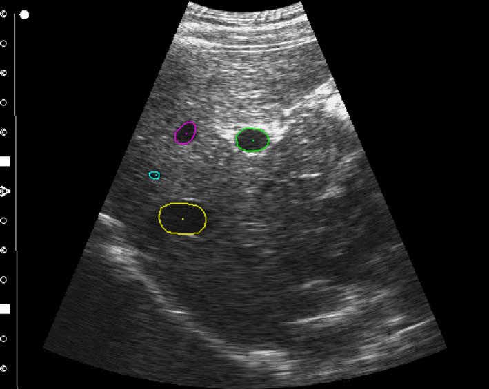
Contour initialization. The initialized first frame contours for the MED‐07‐4 image sequence. The outer contour is manually segmented on the first frame to define the boundary points of the features associated with each landmark point. The landmark points to be tracked are indicated by the single point at the center of each feature. While multiple features are shown for visualization, in practice features are tracked one at a time. [Color figure can be viewed at wileyonlinelibrary.com]

In addition to the data used for algorithm validation, algorithm development was primarily based on the CLUST 14 training set data (two sets, five features) and a subset of the CLUST14 test set data (eight sets, 19 features). The image sets used for development were similar in frequency, imaging rate and duration to the data used to validate the algorithm. Algorithm development was performed using a qualitative analysis where the tracked contour was visually monitored with respect to the appearance of the feature. The contour shape relative to the true feature shape was monitored throughout tracking for partial contour deviations (drift of one contour edge from the true boundary), as well as full contour failures. In scenarios where repeated deviations or failures occurred, the algorithm framework or parameters were adjusted to track the contour boundary more accurately while ensuring the modifications did not significantly compromise the tracking of other features. It should also be noted that while algorithm development was almost entirely performed on the development set mentioned, there were modifications to the algorithm after viewing the validation data. However, this was within the rules outlined by the CLUST challenge and there was no annotation data (outside of the first frame) available to the authors before submitting the tracking results to CLUST for final validation.

2.B. Tracking algorithm framework

The algorithm was developed to employ block matching principles while utilizing both information from the previous frame as well as information from a rolling training set. Critical elements of the proposed algorithm include: a global shift calculation to account for gross displacements, a reference frame selection to find the most similar feature from a training set of previously tracked frames, and a localized deformation calculation based on multiple templates to fine‐tune the contour shape. As shown in the general overview of the proposed algorithm in Fig. 2, these elements are used in every frame during tracking. Additionally, a rolling training set is acquired and grown throughout the first K frames of tracking to be used as reference and to aid in contour shape stabilization in future frames. For all comparisons made in the algorithm, the normalized cross‐correlation (NCC) was chosen as a similarity metric where the NCC is given by

$$\begin{array}{cc}& NCC\left(u,v\right)\hfill \\ & =\frac{{\sum }_{x,y}\left[f\left(x,y\right)-{\overline{f}}_{u,v}\right]\left[g\left(x-u,y-v\right)-\overline{g}\right]}{\sqrt{{\sum }_{x,y}{\left[f\left(x,y\right)-{\overline{f}}_{u,v}\right]}^2{\sum }_{x,y}{\left[g\left(x-u,y-v\right)-\overline{g}\right]}^2}}\hfill \end{array}$$ (1)

where $f(x,y)$ is the search image, $g(x,y)$ is the template image, $(u,v)$ is the image shift, and ${\overline{f}}_{u,v}$ is the mean of $f(x,y)$ in the area of the template. The NCC was chosen to obtain a high accuracy when comparing image similarity while limiting the computational complexity such that real‐time speeds could be attained. The NCC is computationally more efficient than many advanced metrics such as mutual information, while also being more accurate and robust than other computationally efficient metrics such as sum of squared differences or sum of absolute differences.³⁷

Figure 2.

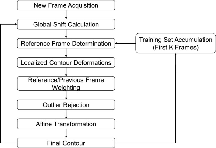
Tracking flowchart. Generalized flowchart of the algorithm framework.

Initialization of the tracking algorithm requires a manual first frame contour be drawn by the user to define the starting point for the feature boundary. The contour drawn by the user is converted to a set of discretized points for tracking by first creating a binary mask of the pixels contained within the contour, and then by using a method based on the Moore‐Neighbor tracing algorithm modified by Jacob's stopping criteria.³⁸ For this work all user defined contours were performed on the first frame of tracking by an author. Examples of the initialized contours are shown in Fig. 1. While four features are shown in the figure to display multiple features at once, in practice features are tracked one at a time and are not simultaneously tracked within an image.

The tracking algorithm is based on tracking the points comprising the feature boundary. As was referenced previously (and will be discussed in more detail in Section 2.B.4.), this is based on the concept of multiple simultaneous templates to provide both shape and temporal constancy. Due to the fact that multiple templates are compared for each boundary point location, it is required that the number of boundary points stay constant throughout tracking and that the location of each boundary point relative to the centroid stay consistent across training images and tracking images. To ensure valid comparison between templates on a point‐by‐point basis, angular normalization is performed at the end of each tracking frame such that the boundary points are always located at distinct angles about the centroid (i.e. 2°, 4°, 6°, etc.). This is achieved by interpolating between the two nearest points in each direction of a given angle.

2.B.1. Training set accumulation

A training set containing information on the feature appearance and contour boundary location is acquired throughout the first K frames of image acquisition. The training set is referenced at later frames and serves as a mechanism to provide feature shape constancy and prevent contour drift. As block matching methods are susceptible to drift over long sequences, the use of a training set helps to provide a shape constraint to the tracking results that is reflective of the expected feature shape as observed in the first K frames of tracking.

At the onset of tracking, the training set only has information for the first frame contour which was initialized by the user. However, for each subsequent frame, the size of the training set grows and the final boundary for each feature is stored in memory. The image data corresponding to each individual feature is cropped such that the tracked centroid of the feature is centered within the image. This allows for all training set images to be aligned, and later facilitates an easier comparison between the tracking frame and all the training frames. Furthermore, as the training frames will be compared to tracking frames that may be acquired at a much later time, it is unlikely that speckle patterns will match between the frames due to decorrelation. Therefore, the intensities related to the speckle pattern are eliminated and a mask image based upon the tracked feature contour is determined. This procedure then allows for a comparison with the training frames on the basis of high contrast light‐to‐dark or dark‐to‐light transitions. The cropped image of the feature will later be used for reference frame selection and smaller templates centered at each boundary point will be used for localized deformation calculations. To avoid repetitive calculations and enhance the speed of future NCC calculations involving the training images, sum tables are obtained of the cropped image intensities and stored in memory as suggested by Luo and Konofagou.³⁹

Initial implementation utilized a training set of K = 200 frames for all sequences analyzed, which corresponded to roughly 2–4 breathing cycles depending on the imaging and respiratory rate. The number of training set frames was set to encompass much of the expected motion and deformation of the feature throughout the subsequent frames, while remaining sufficiently small to avoid the introduction of unnecessary computational complexities.

2.B.2. Global shift calculation

As each new frame of the sequence is acquired, a global shift calculation is performed to manage gross displacements of the feature from the previous frame. The global shift magnitude is calculated by performing NCC‐based block matching in which a template containing the expected feature location in the current frame is scanned through a larger search range in the previous image. The template size of the current image is a fixed size throughout all frames of tracking and is given by

$$T_{Global}=W_{Feat}+\frac{T_{Local}}{2}+d_{Max,Local}+10$$ (2)

where T _Global and T _Local are the global and local template sizes respectively, W _Feat is the diameter of the feature, and d _Max,Local is the maximum local motion during a given frame. The template size is set such that it fully contains the feature plus an additional boundary to allow for feature scaling or shifting over time. The template is then scanned through a search range in the previous image that is larger in size than the template image to allow for a constant 51 × 51 pixel (25 pixel maximum shift) search grid for all features. The fixed search range size is set to encompass the expected maximum frame to frame motion. Both the template image and the search image are centered at the calculated centroid of the previous frame such that a maximum NCC score at the center of the search grid would correspond to zero global motion from the previous to the current frame.

The location in the search grid corresponding to the highest NCC score is taken as the global shift from the previous frame to the current frame given that the NCC was above a user defined threshold (0.55). The threshold was chosen based upon qualitative analysis of training set images by visually assessing the times in which significant shifts were missed between frames. In the case that there is not a good match between the previous and the current frame, it is likely that there has been a substantial change in the feature appearance. Therefore, to attempt to still locate the feature with a high degree of certainty, a previously well‐matched training image, followed by the initial frame, is used in the global shift procedure described above. There is still no guarantee that the training image or initial image will have a similar appearance to the current feature; thus, if all three global searches have a maximum of less than the threshold, the maximum across all three is used to define the global shift. The general process of the globalized matching is presented in the first module of Fig. 3.

Figure 3.

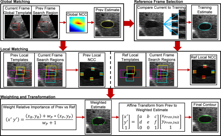
Single frame tracking procedure. A detailed flow diagram outlining the procedure taken to track each frame. The flowchart is broken down into four modules, each corresponding to Sections 2.B.2., 2.B.3., 2.B.4., 2.B.5.. The first module outlines the global matching in which a template set on the current frame is scanned through a search region in the previous frame to find the gross shift of the entire feature. The second module uses the result of the first module and then compares the current image to all images in the training set to determine a most similar training set image. The third module then uses the results of the global matching and reference frame selection to perform localized matching with smaller templates to fine tune the contour shape. The templates are initialized at the boundary points of either the previous or reference frames. Note that only four templates are shown in the image, but in practice they are located at every boundary point. Finally, the two estimates are combined using a weighting scheme on a point‐by‐point basis and an affine transformation is calculated based on the estimated boundary points relative to the previous frame contour to determine the final tracked contour for the current frame. [Color figure can be viewed at wileyonlinelibrary.com]

2.B.3. Reference frame selection

The globalized shift provided a rough estimate of the feature boundary based upon the previous frame; however, in the framework presented it is desired to also use the acquired training set information to provide a degree of shape constancy and obtain a second estimate of the feature boundary. This is done by determining the training set image most similar to the current image based on NCC. The current image is cropped and centered (centering based on global shift calculation in Section 2.B.2.) about the feature and then compared to every image in the training set. The current image and the training set images are the same size and thus there is no scanning needed, and only a single NCC calculation is done for each training set image. The most similar training set image corresponds to the highest NCC given it is above a user defined threshold (0.2). The threshold for the reference frame selection is set based on qualitative analysis of previously tracked features. It is set to a relatively low NCC value to promote matching such that a usable reference frame is found and to account for the fact that the training images have often been acquired much earlier than the current image, making it less likely that the speckle patterns will match well enough to achieve a very high NCC value. This reference frame selection is demonstrated in the second module of Fig. 3.

In the scenario when there is no image in the training set with a similarity above the threshold, it is likely that the feature is not centered properly, and thus a previously well‐matched training image is scanned through a larger section of the current image to determine if the feature has been shifted. If a representative training image still cannot be found after scanning the current image, a reference frame is not selected. Due to the fact that the subsequent steps rely on having both an estimate from the previous frame as well as from the reference frame, if there is no reference frame selected, the tracking for the given frame is terminated at this point and the final contour for the frame is the result of the global shift discussed previously.

2.B.4. Localized matching with multiple templates

By globally aligning the current frame with the previous frame and by also determining the most similar training set image, two rigid estimates of the feature boundary in the current frame are obtained. To account for localized deformations that may occur in the contour boundary, block matching is performed with localized templates for both the masked reference frame and the previous frame independently relative to the current frame. The matching is performed at each boundary point along the contour of the feature. The templates are initialized in either the previous frame or the reference frame at each boundary point location and then are scanned across a search range in the current image. The search region in the current image is centered at the location corresponding to the given boundary point in the previous or reference frame. The localized template sizes and search ranges used for a given feature were determined as linear functions of the number of boundary points in the initial contour, with a larger number of boundary points corresponding to a larger local template size. Template sizes range between 9 × 9 and 41 × 41 pixels, while search ranges varied between 7 × 7 and 11 × 11 pixels. The linear dependence on the number of points was used such that template sizes were relatively consistent with respect to the feature size and to ensure that the localized templates were a subunit of the feature.

As was mentioned previously, the localized reference frame calculations are performed using a mask image to focus on finding high gradient regions that correspond to the feature boundary, and not on matching the background speckle pattern that could be subject to decorrelation. This is demonstrated in the third module of Fig. 3 in which the localized template initializations about the feature boundary are shown for both the previous and reference mask images. While only four of the localized blocks are shown in the figures for clarity, in practice there is a template positioned at every boundary point. By finding the best matching location in the current frame of each template from the previous and reference frames, two estimates of the final boundary after accounting for localized displacements are obtained.

2.B.5. Estimate combination and transformation

At this point the goal is to combine the two boundary estimates to determine a single boundary for the current frame. This is achieved by analyzing the local estimates on a point‐by‐point basis and calculating a weighted sum of the expected boundary locations from the previous and training frames. The single estimate for each boundary point location can then be described by

$$\left(x_m^{\prime },y_m^{\prime }\right)=\frac{(x_{m,Ref},y_{m,Ref})+w_{m,Prev}\ast (x_{m,Prev},y_{m,Prev})}{w_{m,Prev}+1}$$ (3)

where m is the boundary point number, $(x_m^{\prime },y_m^{\prime })$ is the weighted boundary point, $(x_{m,Ref},y_{m,Ref})$ and $(x_{m,Prev},y_{m,Prev})$ are the estimated boundary point location based on the reference and previous estimates respectively, and w _m,Prev is the weight of the previous estimate relative to the reference estimate. The weight of the previous result compared to the reference result is determined for each independent boundary point based upon the matched NCC values, with better matches being weighted more heavily. The one‐to‐one point correspondence between the previous and training frames necessary for the point‐wise analysis is achieved through the angular normalization described in Section 2.B.. The new set of weighted boundary points is then analyzed for possible outliers on the basis of low NCC scores (0.1 reference, 0.92 previous), large angular movements, or large differences between the training and previous matches. The NCC cutoffs used were primarily based on qualitative analysis of times in which the algorithm struggled to correctly identify feature boundaries. For instance, the NCC cutoff relative to the previous frame is primarily based on algorithm performance near regions of shadowing, where at lower cutoffs the algorithm had the potential to fail to detect outliers that had incorrectly extended into the neighboring shadowing regions.

Ultimately, the final contour is determined by calculating the affine transformation from the previous frame contour to the new weighted estimate for the current frame. This transformation is given by

$$\left[\begin{array}{c}{x}^{\prime }\\ y^{\prime }\\ 1\end{array}\right]=\left[\begin{array}{ccc}a& b& c\\ d& e& f\\ 0& 0& 1\end{array}\right]\left[\begin{array}{c}{x}_{Prev,Init}\\ y_{Prev,Init}\\ 1\end{array}\right]$$ (4)

where $(x^{\prime },y^{\prime })$ is the weighted boundary points and (x _Prev,Init , y _Prev,Init ) is the previous contour's initial boundary points. A least squares approach is used to determine the most appropriate transformation from one set of points to the other. The determination of the affine transformation is performed with the outlier points having been removed from both boundary point sets. The estimated affine transformation can then be applied to the full set of previous boundary points (previously determined outliers included) to obtain the final contour in which the total number of boundary points is the same as all previous frames.

2.C. GPU implementation

To enhance the image processing speed and take advantage of the fact that the proposed algorithm is parallelizable, the block matching algorithm was implemented on a graphics processing unit (GPU). The main algorithm was written in MATLAB; however, several MATLAB executable (mex) files calling OpenCV functions or custom CUDA kernels were implemented. The CUDA kernels were written to take advantage of the computational capabilities of a GPU and to address the repetitive NCC calculations which arise in the reference frame selection and localized matching.

The calculations associated with the reference frame selection are rather straight forward, as the current image is directly compared to each static training image of the same size. Thus, there is no translation of the template image and simply 200 static NCC calculations are performed. This is performed on the GPU by first utilizing a kernel to perform the pixel‐wise multiplications associated with the NCC numerator. Then, a separate kernel is used to fully calculate the NCC between the current image and each possible training image, where each training image is calculated with an independent thread. Conversely, detection of the localized templates requires a dynamic shifting of the template image within the search image. Therefore, a different kernel structure is implemented for the localized matching in which each kernel block is associated with a distinct boundary point, and each kernel thread is associated with a possible displacement within the search range of the given boundary point. Subsequently, the optimum location of the localized template corresponding to each boundary point is determined using independent threads for each boundary point.

2.D. Tracking algorithm validation

For each feature of interest, the centroids of the tracked contours were determined at every frame and the net displacement of those centroids relative to the initial contour centroids were calculated. As the goal was to track the specific point‐landmarks annotated by the CLUST organizers, the net displacements of the contour centroids were used to infer the motion of the point‐landmarks. This was done in a manner that assumes the same net displacement between frames for both the contour centroid and the point‐landmarks. Due to the fact that the point‐landmarks roughly corresponded to the feature centroid in all cases, this was considered to be a valid approach. The average difference between the contour centroid after initialization and the first frame point‐landmark annotation was < 0.5 mm, which is on the order of the expected interobserver annotation variability (0.5–0.6 mm) reported by De Luca.³¹ The results of the inferred point‐landmarks were then compared to ground truth as annotated by the CLUST organizers and the Euclidean distance of the inferred point‐landmark from ground truth was used to characterize the performance.

Timings of the algorithm processing speed were performed using the average of three independent runs of the same feature with the image sets preloaded into memory. The primary timings reported in this work are associated with the GPU implemented version of the algorithm. Additionally, to characterize the relative speedup obtained by using a GPU as opposed to a CPU for the reference frame selection and localized matching, a comparison to a multithreaded C++ implementation was explored. All validation testing was performed using an Intel Xeon E5‐2609 2.40 GHz CPU with 1 TB memory and using a Tesla M2090 GPU card with 6 GB GDDR5 memory and 512 CUDA cores.

3. Results

A summary of the overall performance as well as the performance for each sequence subset (different acquisition location and scanner) is provided in Table 1. Values are provided for the total number of features for each subset as well as the mean, standard deviation, 95th percentile, and maximum tracking errors. A full breakdown of the tracking including the mean, standard deviation, and maximum error for each point‐landmark can be found in supporting information. Additionally, Fig. 4 provides the mean tracking accuracy for all features relative to the number of points in the initialized contour.

Table 1.

Tracking performance summary. A summary of the overall performance of the algorithm on all the features tested. Each sequence type represents a different scanner that the sequences were acquired from and the number of features is the total across all sequences for a given scanner. Additionally, the mean, standard deviation, 95th percentile, and maximum tracking accuracies are presented

Sequence	No. Feat.	Mean (mm)	St. dev. (mm)	TE 95th (mm)	Max (mm)
CIL	6	0.89	0.87	2.45	8.58
ETH	30	0.65	1.46	1.43	24.30
ICR	13	0.78	1.27	1.81	11.00
MED1	27	0.86	0.79	2.11	10.34
MED2	9	0.74	0.53	1.71	4.48
2D	85	0.72	1.25	1.71	24.30

Figure 4.

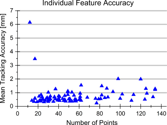
Individual feature tracking accuracy. The mean tracking accuracy is shown for all features analyzed with respect to the number of points in the initialized contour. Tracking failure (Tracking Error > 2.0 mm) was observed in three features with the worst two tracking errors occurring for small features with a low number of boundary points. [Color figure can be viewed at wileyonlinelibrary.com]

Overall the algorithm displayed a mean accuracy of 0.72 ± 1.25 mm across the 85 features analyzed. The average accuracy observed would be sufficient for tracking in radiation therapy and is in line with current state‐of‐the‐art tracking methods. With respect to a 2.0 mm tracking accuracy threshold (as is used in work by O'Shea²⁹), successful tracking was observed for 82 of the 85 features, with 6.14 mm being the worst tracking error observed. The largest tracking error was a result of the algorithm detecting a similar nearby feature and detecting that feature as opposed to the feature of interest. Noting Fig. 4, the two largest tracking errors observed occurred in features with a small number of boundary points, indicating the potential for the algorithm to struggle for smaller features. Additionally, it was observed that tracking of the feature contour performed well for features that had distinct boundary edges; however, there was susceptibility for the tracking to struggle maintaining a consistent contour on features that lacked distinct boundary edges. Relatively consistent results were seen throughout all subsets of data. The average accuracy per scanner subset ranged between 0.65 and 0.89 mm. The consistency across scanners demonstrates the minimal performance dependence on the scanner or transducer used and the potential of the algorithm to be applied across multiple systems.

The processing speed was analyzed during the training set accumulation and postaccumulation independently on a per feature basis with the image sequences preloaded into memory. The processing speeds observed per frame per feature object ranged from 41 to 165 frames per second (fps) during accumulation of the training phase, and from 73 to 234 fps postaccumulation. The processing speed exceeded the imaging rate of the associated acquisition for all sequences. As shown in Fig. 5(a), processing speeds were determined to be dependent upon the overall number of boundary points in the initialized contour, with speeds decreasing with increasing number of points.

Figure 5.

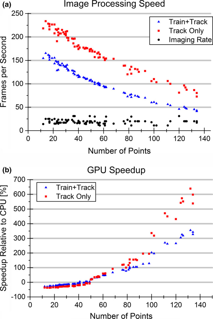
GPU image processing speed. The image processing speed in frames per second for the GPU implementation of the algorithm as a function of the number of points in the initial contour is presented and compared to the imaging rate in (a). The image processing speed decreased with increasing contour size. The relative speedup obtained by implementing the reference frame selection and localized matching calculations on the GPU as opposed to an OpenMP CPU based approach is shown in (b). As the initial contour size increased so did the observed speedup. [Color figure can be viewed at wileyonlinelibrary.com]

Implementation of the algorithm using a GPU for reference frame selection and localized matching calculations resulted in speedups between −30% and 355% during training set accumulation, and −37% and 639% postaccumulation relative to a multithreaded C++ implementation. The observed speedup on a per feature basis is presented in Fig. 5(b). It was observed that GPU implementation did not always perform better, as the CPU implementation performed at a faster rate for small features; however, for large features the GPU implementation greatly outperformed the CPU implementation where a speedup of greater than 600% was observed. The CPU implementation performed better for features containing a smaller number of points as the computational load remained relatively low, and thus the GPU speedup was offset by the overhead associated with copying the data from the hard drive to the GPU memory, and vice versa. The point at which the GPU implementation became advantageous and the relative speedup became positive occurred when the feature size reached approximately 50 boundary points.

4. Discussion

This work presented an algorithm for the 2D tracking of features in ultrasound for the purposes of image guidance during a radiation therapy procedure. A training set of feature information was accumulated over the first K = 200 frames of tracking in an attempt to help negate drift and provide shape constancy to the tracked contour. Obtaining the accumulated training set in turn enabled the simultaneous use of information from both the previous frame (temporal constancy) and a training frame (shape constancy) to consistently track features of interest. Furthermore, the localized block matching was performed using boundary point initialization to enable a search based on boundary edges and high contrast regions as opposed to speckle patterns which can decorrelate over time.

As block matching in general is not a new concept, this work is clearly not the first to implement the general principles for the purposes of ultrasound tracking, and thus this work drew off of several principles of similar works. For instance, the globalized matching step in Section 2.B.2. is quite simply a naïve correlation‐based block matching approach where the previous frame is always used as reference (in our case with the template encompassing the entire feature). Correlation‐based block matching has been applied in several other works, either as the primary focus, or simply as a smaller portion of the overall algorithm.^{24, 25, 26, 28, 29, 30, 40} It has been shown by both De Luca et al.²⁴ and O'Shea et al.²⁹ that this naïve approach applied by itself performs poorly over long sequences, necessitating the need for additional stabilization techniques to avoid the effects of drift. To address this concern over long sequences, De Luca²⁴ proposed the use of a training set, and Kondo²⁵ took a similar approach as well, in which accuracies of 0.96 mm and 1.71 mm were reported respectively. Methods outlined in Section 2.B.3. make use of a training set and the selection of a reference frame which is similar to the works of De Luca and Kondo. However, while a few of the underlying concepts are derived from other works, what distinguishes this work from these previous approaches and allowed for advances in accuracy include the training set accumulation, the simultaneous use of multiple templates on each frame, and the use of a mask image for the localized matching along the boundary of the contour.

In this work, a training set was accumulated from the tracking results of the first K = 200 frames without the use of a pretreatment scan. Theoretically the size of the training set could be adjusted to accommodate a variable number of breathing cycles; however, there will be a tradeoff between encompassing more of the projected motion scenarios and the added computations to extend the training set size. By obtaining the training set from the initial tracking results, the necessity of a pretreatment scan, or a pure learning phase, was eliminated, which could potentially lead to more accurate tracking as well as a more suitable clinical workflow. Obtaining the training set from the first several frames of tracking will limit the potential for any gross displacements of the transducer or patient anatomy between the training set acquisition and the beginning of tracking, and will likely allow for a more representative training set of the true feature shape and orientation expected. Additionally, by utilizing the first subset of the frames acquired, we obtain the training set of information in a timeframe at which the tracking is the most accurate. If the training information were taken or updated at later times in the tracking sequence, there is a greater probability of drift or error accumulation, resulting in poor representation of the true feature shape. This is of importance as there is no way to truly validate whether a contour is correct or not during the tracking procedure and thus it is essential to acquire this training set during the time at which the tracking is expected to be most accurate.

Additionally, this work utilized multiple templates simultaneously for each frame as opposed to choosing a single template from a set of possible options. Since boundary point‐to‐point correspondence between the previous and training frames was obtained by normalizing the boundary points at set angles about the centroid, analysis could be performed on a boundary point‐wise basis. Theoretically the corresponding boundary points in both templates are trying to find the same boundary points in the current image, thus the results could be compared to obtain a weighted average with information from both the previous and a training image. A single reference frame can either provide temporal constancy (previous frame) or shape constancy/renormalization (training frame) to the tracked contour. Our approach was able to simultaneously use both templates in order to provide temporal and shape constancy at each frame. Another advantage of this approach was that it enabled the better detection of potential outlier boundary points as the position of a given boundary point based on each template could be compared on an absolute scale. If a large difference was seen between the previous frame's match and the training frame's match, the boundary point could be removed when calculating the transformation since it was likely unrepresentative of the true boundary.

Finally, by performing the block matching at localized regions surrounding each of the contour boundary points, the templates were able to be initialized at strategic locations on feature edges. Positioning the templates along the feature edges allowed for the use of the most relevant and easily distinguishable information for each feature by emphasizing high contrast regions of the image as opposed to pure speckle patterns. Boundary point block initialization has been done in the past by Boukerroui;²⁷ however, in this work it was coupled with the use of a training set mask image. Finding blocks that contained boundary edges greatly enhanced the performance of the algorithm, especially when finding matches from the training set mask images. As it was likely that the training data was taken at times much different than the analysis frame, it could not be reasonably expected for the speckle pattern to be consistent. Due to out of plane motion as well as nonuniform movement of scatterers, the speckle pattern in 2D images has been known to decorrelate over time.⁴¹ Therefore, trying to find blocks from a comparison image which contains a large degree of speckle pattern and was taken at a time much earlier than the analysis image is not always valid, and could lead to poor results. Therefore, by eliminating all dependence on the speckle pattern and using a mask of the training images, a more representative match could potentially be found in the tracked frame.

Our results have shown how the addition of these novel aspects of the algorithm have allowed for the accurate tracking of point‐landmarks within ultrasound sequences. The accuracy reported is comparable to or exceeds alternative 2D tracking methods. The mean tracking error of ±0.72 mm compared favorably with other algorithms applied to the CLUST 15 data set, with the next closest algorithm presenting a mean tracking error of ±1.21 mm.²² However, there are differences between how this method and other methods were applied to the CLUST 15 data that are noteworthy. This approach was developed after the on‐site challenge concluded, implying that access to all data was allowed before computation as opposed to only 80% of the data for those participating in the on‐site challenge. Additionally, our method relied on a first frame initialized contour as opposed to a single point landmark initialization. However, the method submitted was still within the rules outlined by the CLUST as all parameters were either automatically determined or fixed across all sequences, ensuring that the algorithm was not optimized for each individual sequence.

While the algorithm performed extremely well for the overall feature set, several limitations were observed throughout the development and testing of the algorithm that will need to be addressed moving forward. It was observed that the algorithm may be at a disadvantage when encountering extremely small features, poorly defined feature boundaries, and nonconvex features. As shown in Fig. 4, the two worst tracking performances observed were for features with a limited number of boundary points in the initialized contour. While theoretically the algorithm should still work with a limited number of boundary points, the effects of an undetected outlier have a much greater chance of producing inaccurate results than it would for larger features. With a smaller number of boundary points, each boundary point carries a greater weight, meaning a single poor match can greatly impact the entire contour and cause it to lose the true feature. Relatively poor performance was also observed in features with poorly defined feature boundaries, for instance if a feature has a very bright top and bottom edge however the lateral edges of the feature tend to slowly transition to speckle. This can especially be of concern for matching with the reference frame which strongly depends on the high contrast regions at feature boundaries. Because there was poor definition of feature edges, many of the points near these regions were either removed as outliers due to poor matches or matched to a high contrast neighboring structure, leading to large variability of the contour. While ultimately the well‐defined regions of each individual contour allowed for reasonable point‐landmark tracking, the large variability at regions that did not exhibit large intensity gradients led to a worsened contour estimation and a decreased accuracy. The degree to which this effect is observed could be impacted by the image compression used before analysis. For this work the images were provided to the user in PNG format, a lossless compression method, and thus minimal effect was expected. However, had the data been analyzed based on a lossy compression method, such as JPEG, there could have been a loss of details in the low contrast regions and a potential negative impact on the algorithm performance. While it was not demonstrated in the features analyzed in the work, a further limitation of the algorithm is the current inability to handle grossly nonconvex feature sets. To analyze the best match from the previous frame and a training frame, and compare them to each other on a point‐wise basis, an angular regularization of the contour boundary points was adopted into the framework as was discussed in Section 2.B.. This ensured that the same number of boundary points was always present, and that the boundary points for both the previous and training frames occurred at the same angles about the centroid. However, this angular regularization approach is only applicable for convex, or very nearly convex features. In the event of a nonconvex contour, there is the potential for multiple occurrences of a given angle, thus allowing for potential inaccuracies and multiple answers during the angular interpolation. This shortcoming is not represented in the accuracy presented as all features were either convex, or very nearly convex such that the issue did not arise. However, as we are aware of the potential for nonconvex features in practice, investigation into an alternative approach applying deformable registration between consecutive mask images to establish point correspondence is also being explored.

The algorithm processed the image data at speeds (41–165 fps training accumulation, 73–234 fps postaccumulation) that exceeded the imaging rate (11–31 fps) for each ultrasound sequence. Since this work was performed using a set of retrospective ultrasound sequences, the data transfer latency from the imaging unit to an external processing unit is unknown. However, the degree to which the image processing speeds exceeded standard 2D imaging rates provided confidence that the algorithm has the potential to be used for real‐time application. The observed image processing speed also showed the effectiveness and necessity of applying the algorithm on a GPU. When the algorithm was implemented on the CPU only, it was observed that the average speeds failed to reach real‐time rates for 8 of the features. Failure to reach the real‐time rate could then lead to an increasing latency of triggering the beam on or off relative to the image acquisition over time, or necessitate the skipping of frames to allow for the analysis to keep up with the image acquisition. The GPU implementation proved to enhance the parallelizable calculations, as speed increases between −30% and 355% during training set accumulation, and −37% and 639% postaccumulation were observed. With a GPU, real‐time rates were reached for all features, a substantial improvement in performance. Not only is this significant because it allows for processing at a rate equal to or faster than acquisition to avoid buildup of images, but it is also significant with respect to the overall motion management system latency. The latency of an MLC tracking system is composed of the image acquisition, processing, and MLC repositioning speeds. Sawkey et al. has shown that system latency is the dominant source of positional uncertainty when applying MLC tracking and that a reduction in latency from 200 ms to 100 ms can lead to a reduction in necessary margins from 4.6 mm to 3.1 mm.⁴² The decrease in margins would then subsequently decrease the normal tissue dose while still delivering an adequate dose to the target. Therefore, if the largest feature seen in this work (134 boundary points) is considered, the average processing speed is reduced from 88 ms to 13 ms by implementing the algorithm on the GPU as opposed to the CPU, resulting in an overall decrease in system latency of 75 ms, which could be significant in terms of margin reduction. It was also demonstrated that the effectiveness of the GPU was enhanced with a greater number of necessary calculations, as Fig. 5(b) demonstrates an increase in speedup with increasing number of points. With this in mind, as the work is expanded to 3D, it is expected that the GPU implementation will become more useful and provide an even greater speedup due to the added calculations and increased number of boundary points that will come with an added dimensionality.

While this work focused solely on the tracking of liver vessels from retrospective ultrasound image sets, the desire is for the algorithm to eventually be applied in a clinical setting. With this in mind, it is important to consider the potential impact a clinical situation may have on the algorithm performance, as well as alternative applications. As has been mentioned, the algorithm relies on a manual first frame contour initialization. In the setup used in this work, the contour was initialized on the first frame and tracking consequently began at the next acquired frame. However, clinically the time latency between contour initialization and the beginning of tracking will be much longer than the time between consecutive images. This effect has not yet been explored, however, will likely rely on either patient breath‐hold during contour initialization, or frame matching to ensure that the feature is at a similar location relative to the initial contour when tracking begins. Additionally, this work focused on the tracking of liver vessels, however clinically the PTV is more often of interest. In an ideal scenario, the tracking algorithm could simply be used to directly track the PTV if it is visible in the ultrasound image. However, in the case where the PTV is not visible on the ultrasound image, the liver vessels proximal to the tumor target will generally be used as a surrogate to estimate PTV position. Therefore, the overall clinical effectiveness of the tracking approach will not only rely on the tracking of the vessels, but additionally on the mapping accuracy between the vessels and the PTV. Additionally, the clinical impact of the algorithm implementation does not have to be limited to ultrasound, as it could be applied to alternative imaging modalities such as MRI with systems such as the ViewRay MRIdian^® or future MR‐linac systems. Preliminary investigations into the tracking of both liver vessels and lung tissue with MRI have shown favorable results, and the possibility of direct tumor tracking with applied contrast agents is a potential future application.

5. Conclusions

This work implemented a 2D block matching algorithm while simultaneously using multiple templates to retrospectively track point‐landmarks in ultrasound sequences. We have implemented the use of a rolling training set as a method to retain information about features throughout several initial breathing cycles and to aid in subsequent tracking of the features. Through the simultaneous use of training set images and the previous image we were able to provide both shape and temporal constancy to aid in the consistent tracking of feature contours, and subsequently point‐landmarks, throughout long ultrasound sequences. The high accuracy (±0.72 mm) and image processing speed (41–165 fps training accumulation, 73–234 fps postaccumulation) exhibited have demonstrated the potential of the algorithm to be used as an effective real‐time tracking approach for radiation therapy.

Conflict of interest

The authors have no relevant conflicts of interest to disclose.

Supporting information

Table SI. Full Tracking Performance. A full summary of the tracking performance on each feature tested from the CLUST 15 data set. The mean, standard deviation and maximum error are presented for each feature.

References

- 1. Keall PJ, Mageras GS, Balter JM, et al. The management of respiratory motion in radiation oncology report of AAPM Task Group 76. Med Phys. 2006;33:3874–3900. [DOI] [PubMed] [Google Scholar]
- 2. Son SH, Choi BO, Ryu MR, et al. Stereotactic body radiotherapy for patients with unresectable primary hepatocellular carcinoma: dose‐volumetric parameters predicting the hepatic complication. Int J Radiat Oncol Biol Phys. 2010;78:1073–1080. [DOI] [PubMed] [Google Scholar]
- 3. Goyal S, Kataria T. Image guidance in radiation therapy: techniques and applications. Radiol Res Pract. 2014;2014:705604. [DOI] [PMC free article] [PubMed] [Google Scholar]
- 4. Higgins J, Bezjak A, Hope A, et al. Effect of image‐guidance frequency on geometric accuracy and setup margins in radiotherapy for locally advanced lung cancer. Int J Radiat Oncol Biol Phys. 2011;80:1330–1337. [DOI] [PubMed] [Google Scholar]
- 5. Wagman R, Yorke E, Ford E, et al. Respiratory gating for liver tumors: use in dose escalation. Int J Radiat Oncol Biol Phys. 2003;55:659–668. [DOI] [PubMed] [Google Scholar]
- 6. Poulsen PR, Worm ES, Hansen R, Larsen LP, Grau C, Høyer M. Respiratory gating based on internal electromagnetic motion monitoring during stereotactic liver radiation therapy: first results. Acta Oncol. 2015;54:1445–1452. [DOI] [PubMed] [Google Scholar]
- 7. Worm ES, Høyer M, Fledelius W, Poulsen PR. Three‐dimensional, time‐resolved, intrafraction motion monitoring throughout stereotactic liver radiation therapy on a conventional linear accelerator. Int J Radiat Oncol Biol Phys. 2013;86:190–197. [DOI] [PubMed] [Google Scholar]
- 8. Lagendijk JJ, Raaymakers BW, van Vulpen M. The magnetic resonance imaging‐linac system. Semin Radiat Oncol. 2014;24:207–209. [DOI] [PubMed] [Google Scholar]
- 9. Gierga DP, Brewer J, Sharp GC, Betke M, Willett CG, Chen GT. The correlation between internal and external markers for abdominal tumors: implications for respiratory gating. Int J Radiat Oncol Biol Phys. 2005;61:1551–1558. [DOI] [PubMed] [Google Scholar]
- 10. Patel A, Khalsa B, Lord B, Sandrasegaran K, Lall C. Planting the seeds of success: CT‐guided gold seed fiducial marker placement to guide robotic radiosurgery. J Med Imaging Radiat Oncol. 2013;57:207–211. [DOI] [PubMed] [Google Scholar]
- 11. Kim JH, Hong SS, Park HJ, Chang YW, Chang AR, Kwon SB. Safety and efficacy of ultrasound‐guided fiducial marker implantation for CyberKnife radiation therapy. Korean J Radiol. 2012;13:307–313. [DOI] [PMC free article] [PubMed] [Google Scholar]
- 12. Murphy MJ, Balter J, Balter S, et al. The management of imaging dose during image‐guided radiotherapy: report of the AAPM Task Group 75. Med Phys. 2007;34:4041–4063. [DOI] [PubMed] [Google Scholar]
- 13. Elekta. Elekta plans to introduce MRI‐guided radiation therapy system in 2017. https://www.elekta.com/meta/press-all.html?id=970154. Accessed November 29, 2016. [Google Scholar]
- 14. Fontanarosa D, van der Meer S, Bamber J, Harris E, O'Shea T, Verhaegen F. Review of ultrasound image guidance in external beam radiotherapy: I. Treatment planning and inter‐fraction motion management. Phys Med Biol. 2015;60:R77–R114. [DOI] [PubMed] [Google Scholar]
- 15. O'Shea T, Bamber J, Fontanarosa D, van der Meer S, Verhaegen F, Harris E. Review of ultrasound image guidance in external beam radiotherapy part II: intra‐fraction motion management and novel applications. Phys Med Biol. 2016;61:R90–R137. [DOI] [PubMed] [Google Scholar]
- 16. Hsu A, Miller NR, Evans PM, Bamber JC, Webb S. Feasibility of using ultrasound for real‐time tracking during radiotherapy. Med Phys. 2005;32:1500–1512. [DOI] [PubMed] [Google Scholar]
- 17. Zhong Y, Stephans K, Qi P, Yu N, Wong J, Xia P. Assessing feasibility of real‐time ultrasound monitoring in stereotactic body radiotherapy of liver tumors. Technol Cancer Res Treat. 2013;12:243–250. [DOI] [PubMed] [Google Scholar]
- 18. Bednarz B, Culberson W, Bassetti M, et al. A real‐time tumor localization and guidance platform for radiotherapy using US and MRI. American Association of Physicists in Medicine 2016 Annual Meeting. Washington, DC, USA; 2016.
- 19. Foo T, Culberson W, Bassetti M, et al. Image guided radiation therapy using combined MRI and ultrasound. National Image Guided Therapy Workshop; 2016.
- 20. Cao K, Bednarz B, Smith LS, Foo TKF, Patwardhan KA. Respiration Induced Fiducial Motion Tracking in Ultrasound Using an Extended SFA Approach. SPIE Medical Imaging. Orlando, Florida, USA; 2015.
- 21. Konig L, Kipshagen T, Ruhaak J. A Non‐Linear Image Registration Scheme for Real‐Time Liver Ultrasound Tracking using Normalized Gradient Fields. MICCAI 2014 Challenge on Liver Ultrasound Tracking. Cambridge, MA, USA; 2014.
- 22. Hallack A, Papiez BW, Cifor A, Gooding MJ, Schnabel JA. Robust Liver Ultrasound Tracking using Dense Distinctive Image Features. MICCAI 2015 Challenge on Liver Ultrasound Tracking. Munich, Germany; 2015.
- 23. Rothlubbers S, Schwaab J, Jenne J, Gunther M. MICCAI CLUST 2014 – Bayesian Real‐Time Liver Feature Ultrasound Tracking. MICCAI 2014 Challenge on Liver Ultrasound Tracking. Cambridge, MA, USA; 2014.
- 24. De Luca V, Tschannen M, Székely G, Tanner C. A learning‐based approach for fast and robust vessel tracking in long ultrasound sequences. Med Image Comput Comput Assist Interv. 2013;16:518–525. [DOI] [PubMed] [Google Scholar]
- 25. Kondo S. Liver Ultrasound Tracking Using Long‐term and Short‐term Template Matching. MICCAI 2014 Challenge on Liver Ultrasound Tracking. Cambridge, MA, USA; 2014.
- 26. Banerjee J, Klink C, Peters ED, Niessen WJ, Moelker A, van Walsum T. Fast and robust 3D ultrasound registration–block and game theoretic matching. Med Image Anal. 2015;20:173–183. [DOI] [PubMed] [Google Scholar]
- 27. Boukerroui D, Noble JA, Brady M. Velocity estimation in ultrasound images: a block matching approach. Inf Process Med Imaging. 2003;18:586–598. [DOI] [PubMed] [Google Scholar]
- 28. Wu J, Li C, Gogna A, et al. Technical note: automatic real‐time ultrasound tracking of respiratory signal using selective filtering and dynamic template matching. Med Phys. 2015;42:4536–4541. [DOI] [PubMed] [Google Scholar]
- 29. O'Shea TP, Bamber JC, Harris EJ. Temporal regularization of ultrasound‐based liver motion estimation for image‐guided radiation therapy. Med Phys. 2016;43:455. [DOI] [PMC free article] [PubMed] [Google Scholar]
- 30. Makhinya M, Goksel O. Motion Tracking in 2D Ultrasound Using Vessel Models and Robust Optic‐Flow. MICCAI 2015 Challenge on Liver Ultrasound Tracking, Munich, Germany; 2015.
- 31. De Luca V, Benz T, Kondo S, et al. The 2014 liver ultrasound tracking benchmark. Phys Med Biol. 2015;60:5571–5599. [DOI] [PMC free article] [PubMed] [Google Scholar]
- 32. Preiswerk F, De Luca V, Arnold P, et al. Model‐guided respiratory organ motion prediction of the liver from 2D ultrasound. Med Image Anal. 2014;18:740–751. [DOI] [PubMed] [Google Scholar]
- 33. Lediju MA, Byram BC, Harris EJ, Evans PM, Bamber JC. 3D Liver Tracking Using a Matrix Array: Implications for Ultrasonic Guidance of IMRT. IEEE International Ultrasonics Symposium – IUS 2010; 2010.
- 34. Bell MA, Byram BC, Harris EJ, Evans PM, Bamber JC. In vivo liver tracking with a high volume rate 4D ultrasound scanner and a 2D matrix array probe. Phys Med Biol. 2012;57:1359–1374. [DOI] [PubMed] [Google Scholar]
- 35. Vijayan S, Klein S, Hofstad EF, Lindseth F, Ystgaard B, Lango T. Validation of a Non‐Rigid Registration Method for Motin Compensation in 4D Ultrasound of the Liver. IEEE 10th International Symposium on Biomedical Imaging; 2013.
- 36. Banerjee J, Klink C, Peters ED, Niessen WJ, Moelker A, Van Walsum T. 4D Liver Ultrasound Registration. International Workshop on Biomedical Image Registration: Biomedical Image Registration, Lecture Notes in Computer Science; 2014.
- 37. Wachinger C, Klein T, Navab N. Locally adaptive Nakagami‐based ultrasound similarity measures. Ultrasonics. 2012;52:547–554. [DOI] [PubMed] [Google Scholar]
- 38. Gonzalez RC, Woods RE, Eddins SL. Digital Image Processing Using MATLAB®, 2nd edn. United States: Gatesmark Publishing; 2009. [Google Scholar]
- 39. Luo J, Konofagou E. A fast normalized cross‐correlation calculation method for motion estimation. IEEE Trans Ultrason Ferroelectr Freq Control. 2010;57:1347–1357. [DOI] [PMC free article] [PubMed] [Google Scholar]
- 40. Harris EJ, Miller NR, Bamber JC, Symonds‐Tayler JR, Evans PM. Speckle tracking in a phantom and feature‐based tracking in liver in the presence of respiratory motion using 4D ultrasound. Phys Med Biol. 2010;55:3363–3380. [DOI] [PubMed] [Google Scholar]
- 41. Yeung F, Levinson SF, Fu D, Parker KJ. Feature‐adaptive motion tracking of ultrasound image sequences using a deformable mesh. IEEE Trans Med Imaging. 1998;17:945–956. [DOI] [PubMed] [Google Scholar]
- 42. Sawkey D, Svatos M, Zankowski C. Evaluation of motion management strategies based on required margins. Phys Med Biol. 2012;57:6347–6369. [DOI] [PubMed] [Google Scholar]
Associated Data
This section collects any data citations, data availability statements, or supplementary materials included in this article.
Supplementary Materials