A combined learning algorithm for prostate segmentation on 3D CT images

Abstract

Purpose

Segmentation of the prostate on CT images has many applications in the diagnosis and treatment of prostate cancer. Because of the low soft‐tissue contrast on CT images, prostate segmentation is a challenging task. A learning‐based segmentation method is proposed for the prostate on three‐dimensional (3D) CT images.

Methods

We combine population‐based and patient‐based learning methods for segmenting the prostate on CT images. Population data can provide useful information to guide the segmentation processing. Because of inter‐patient variations, patient‐specific information is particularly useful to improve the segmentation accuracy for an individual patient. In this study, we combine a population learning method and a patient‐specific learning method to improve the robustness of prostate segmentation on CT images. We train a population model based on the data from a group of prostate patients. We also train a patient‐specific model based on the data of the individual patient and incorporate the information as marked by the user interaction into the segmentation processing. We calculate the similarity between the two models to obtain applicable population and patient‐specific knowledge to compute the likelihood of a pixel belonging to the prostate tissue. A new adaptive threshold method is developed to convert the likelihood image into a binary image of the prostate, and thus complete the segmentation of the gland on CT images.

Results

The proposed learning‐based segmentation algorithm was validated using 3D CT volumes of 92 patients. All of the CT image volumes were manually segmented independently three times by two, clinically experienced radiologists and the manual segmentation results served as the gold standard for evaluation. The experimental results show that the segmentation method achieved a Dice similarity coefficient of 87.18 ± 2.99%, compared to the manual segmentation.

Conclusions

By combining the population learning and patient‐specific learning methods, the proposed method is effective for segmenting the prostate on 3D CT images. The prostate CT segmentation method can be used in various applications including volume measurement and treatment planning of the prostate.

1. Introduction

Prostate cancer is one of the leading causes of cancer mortality in American men. It is estimated that there were 180,890 new cases of prostate cancer in the United States in 2016, and which accounts for 21% of all cases in men.¹ Accurate prostate segmentation on CT images is important for the diagnosis and treatment of prostate cancer. Manual segmentation is time‐consuming and depends on the skill and experience of the clinician. As a result, various efforts have been made to develop segmentation methods for prostate CT images to meet the requirements of clinical applications.² Those methods include atlas‐based approaches, level‐sets, genetic algorithms, and deformable shape models.^{3, 4, 5, 6, 7, 8, 9, 10, 11, 12, 13} Since CT images have low soft‐tissue contrast, learning methods with prior knowledge can be useful to aid in the segmentation of a new patient data. Learning‐based segmentation methods can be divided into three categories.

The first category of learning‐based segmentation methods is to ascertain a patient‐specific model for the prostate segmentation of the same patient. As the variations in prostate size and shape are small regarding the image data acquired from the same patient, the model learned from the images in the same patient can guide the prostate segmentation. Wu et al.¹⁴ utilized the latest image information of the current patient to construct the dictionary for the segmentation of a new image. Shi et al.^{15, 16} proposed spatial‐constrained transductive Lasso to generate a 3D prostate‐likelihood map. They used previous images to obtain the shape information to obtain the final segmentation of the prostate in the current image. Liao et al.¹⁷ used discriminative, patch‐based features based on logistic sparse Lasso and a new multi‐atlas label fusion method to segment the prostate in the new images. They used the segmented images of the same patient to implement an online update mechanism. Li et al.¹⁸ used the planning image and the previously segmented treatment images to train two sets of location‐adaptive classifiers for the segmentation of the prostate in current CT images. Gao et al.¹⁹ used sparse representation‐based classification to obtain an initial, segmented prostate. They used the previous, segmented prostate of the same patient as patient‐specific atlases, aligned the atlases onto the current image, and adopted a majority voting strategy to achieve the prostate segmentation.

The second category of learning‐based segmentation methods is to derive a population model from the other patients for the segmentation of a new patient. When segmented CT images of the same patient are not available, only population information can be used to guide the prostate segmentation. Martínez et al.²⁰ created a set of prior organ shapes by applying principal component analysis to a population of manually delineated CT images. For a given patient, they searched the most similar shape and deformed the shape to segment the prostate, rectum, and bladder in planning CT images. Gao et al.²¹ learned a distance transform based on the planning CT images from different patients for boundary detection, and integrated the detected boundary into a level set formulation for segmenting the prostate on CT images. Chen et al.²² proposed a new segmentation cost function for the segmentation of the prostate and rectum. The cost function incorporates learned intensity, shape, and anatomy information from the images of other patients. Song et al.²³ incorporated the intensity distribution information learned from other patients into a graph search framework for the segmentation of the prostate and bladder.

The third category of learning‐based segmentation methods is to combine a population learning method and a patient‐specific learning method together. Although population data can provide useful information to guide segmentation processing, due to inter‐patient variations, patient‐specific information is required to improve the segmentation accuracy for an individual patient. Park et al.²⁴ utilized a priori knowledge from population data and the patient‐specific information from user interactions to estimate the confident voxels of the prostate. Based on these confident voxels, they selected the discriminative features for semi‐supervised learning to predict the labels of unconfident voxels. Gao et al.²⁵ proposed a novel learning framework to “personalize” a population‐based, discriminative appearance model, and to fit the patient‐specific appearance characteristics. They used backward pruning to discard obsolete, population‐based knowledge and used forward learning to incorporate patient‐specific characteristics. Liao et al.²⁶ learned informative anatomical features in the training images and current images. An online update mechanism was used to guide the localization process. Park et al.²⁴ used user interactions to select similar images from population data for feature selection. Gao et al.²⁵ and Liao et al.²⁶ used previous images of the same patient to guide the segmentation of new images.

In this study, we combine the population learning and patient‐specific learning together for segmenting the prostate on CT images. Being different from the existing methods, we train a population model based on the data from different patients and we consider different distribution patient‐specific models for the base, mid‐gland, and apex regions of the prostate because one patient‐specific model cannot describe the shape difference among the three regions. We train three, patient‐specific models based on the information marked by the user. We compute the similarity of the population model and three, patient‐specific models to obtain the applicable knowledge for the specific patient, and then use the knowledge for more accurate segmentation of prostate. In our initial study,²⁷ we tested a learning‐based segmentation method in a small number of 15 patients. In the current study, we propose new algorithmic aspects and performed a comprehensive validation study in 92 patients. Each of the CT volumes was segmented three times by two, clinically experienced radiologists. The manual segmentation was used as the gold standard for validation of the learning‐based segmentation.

The main contributions of this manuscript are summarized as follows: (a) We combined population learning and patient‐specific learning methods for segmenting prostate CT images. Our method can maximize the advantage of each learning method and minimize the disadvantage of each method, and thereby can achieve better performance than a pure population learning or pure patient‐specific learning method; (b) We propose a new, adaptive thresholding method to convert the prostate‐likelihood map into a binary image for the prostate segmentation. The case‐specific threshold value further improves the segmentation accuracy; (c) We use the information on the base, mid‐gland, and apex regions of the prostate to train three, patient‐specific models. With the three models, our method not only considers the different distribution in different parts of the prostate, but also incorporates population information from other patients when the previous images are not available from the same patient; and (d) Our method needs the user to select three key slices to build the patient‐specific models for the patient‐specific knowledge, and the result shows that the proposed method is robust to the selections of the apex, base, and middle slices.

2. Method

Our learning‐based segmentation method consists of four components, i.e., feature extraction, population learning and patient‐specific learning, prostate‐likelihood prediction by capturing the population and patient‐specific characters, and adaptively binary prostate segmentation based on the area distribution model. Figure 1 shows the flowchart of the proposed method.

Figure 1.

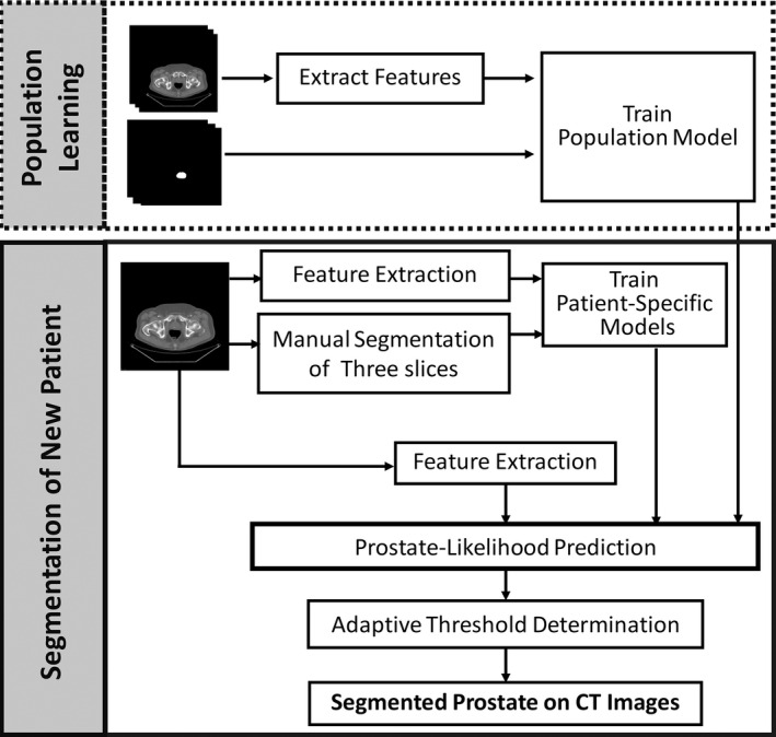
Flowchart of the learning‐based segmentation method for the prostate on 3D CT images.

2.A. Registration

The prostates from different patients have different shapes. To improve classification performance, we align the prostates of different patients in the same orientation and in approximately same location so the features are not affected by the spatial information.

We randomly select one segmented prostate CT images as the fixed image and align other segmented prostates with the fixed one. We use rigid transformation and mutual information and obtain the optimized, transformed images when the registration process reaches the specified maximum number of iterations. We overlay the entire training images together before and after registration, as shown in Fig. 2. The transformed images form a prostate shape or atlas that is helpful for distinguishing between the prostate and non‐prostate pixels, thus improving segmentation performance.

Figure 2.

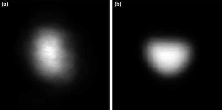
Prostate shape models (a) before and (b) after registration.

2.B. Feature extraction

We used six different types of discriminant features to describe each pixel in the aligned images, including the intensity, multi‐scale rotation Local Binary Pattern (mrLBP), Gray‐Level Co‐occurrence Matrix (GLCM), Histogram of oriented gradient (HOG), Haar‐like features, and the CT value histogram (CThist). Figure 3 shows the six different discriminant image features.

Figure 3.

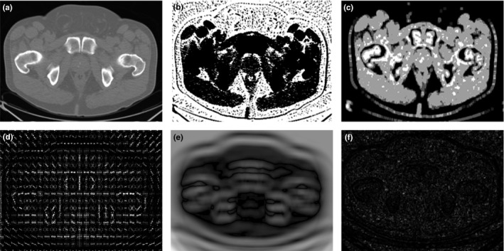
Feature images: (a–f) Original images that are an intensity feature image, mrLBP feature image, GLCM feature image, HOG feature image, Haar‐like feature image, and the CThist feature image.

2.B.1. Intensity

The intensity value is a useful indicator of the local spatial variation in the boundary.

2.B.2. Multi‐scale rotation local binary pattern

The LBP feature²⁸ is a compact texture descriptor in which each comparison result between a center pixel and one of its surrounding neighbors is encoded as a bit. The neighborhood in the LBP operator can be defined very flexibly. We define a rectangle neighborhood, represented by (P, R), where P represents the number of sampling points and R is the radius of the neighborhood. By using the different P and R, we can achieve multi‐scale rotation local binary pattern (mrLBP) features. In addition, for obtaining a stable LBP value, we rotate each bit pattern in each scale to the minimum value and use the minimum as its LBP value. The ranges of P and R for calculating the LBP feature are set to be (4, 8, 16, 24) and (1, 2, 3), respectively. Therefore, we have 8‐D LBP features (when R = 1, P is 4 or 8, when R = 2, P is 4, 8, or 16, and when R = 3, P is 4, 8, or 24). Figure 4 shows the mrLBP for the center pixel, represented by a solid, five‐pointed star. In Fig. 4, the hollow and solid circle represents the comparison result between the center pixel and its surrounding neighbor. The first row gives an example of the multi‐scale LBP feature and the second one shows the mrLBP feature by rotating each bit for a minimum value.

Figure 4.

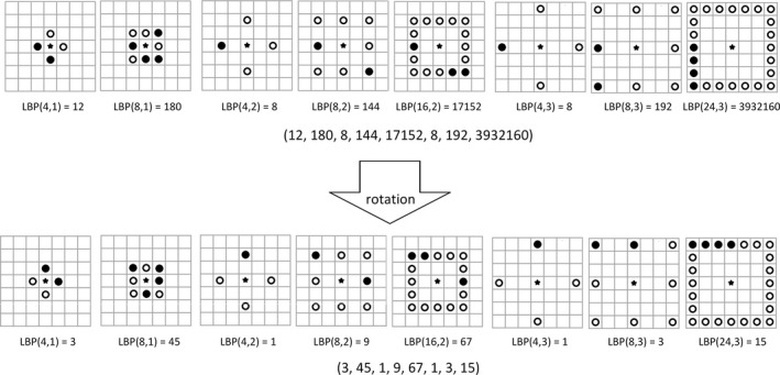
An example of the Multi‐scale Rotation Local Binary Pattern (mrLBP) feature.

2.B.3. Gray‐level co‐occurrence matrix

The gray level co‐occurrence matrix (GLCM)²⁹ is a well‐known statistical tool for extracting second‐order texture information from images. It can deal with the spatial relationships of pairs of gray values of pixels. A co‐occurrence matrix is a function of distance d, angle θ, and grayscales i and j. Its element is specified by the relative frequencies P(i, j, d, θ) in which two pixels, separated by distance d, occur in a direction specified by the angle θ, one with gray level i and the other with gray level j. We compute four GLCM with a distance of one pixel and four directions of 0˚, 45˚, 90˚, and 135˚. For each co‐occurrence matrix, we use four criteria to characterize its statistical behavior, including Energy, Entropy, Contrast, and Correlation. Therefore, we will have the 16‐D GLCM feature from a small 7 × 7 window centered at each pixel. Specifically, Energy is a measure of local homogeneity and it can therefore describe how uniform the texture is. It can be calculated by

$$Energy(d,\mathit{\theta })={\sum }_i{\sum }_j{P}^2(i,j,d,\mathit{\theta }).$$ (1)

Entropy can measure the randomness and spatial disorder of the gray‐level distribution. It can be calculated by

$$Entropy(d,\mathit{\theta })=-{\sum }_i{\sum }_{j}P(i,j,d,\mathit{\theta })·\text{log}(P(i,j,d,\mathit{\theta })).$$ (2)

Contrast is a local grey‐level variation in the grey‐level co‐occurrence matrix. It can be calculated by

$$Contrast(d,\mathit{\theta })={\sum }_i{\sum }_j{(i-j)}^2·P(i,j,d,\mathit{\theta })$$ (3)

Correlation measures the joint probability occurrence of the specified pixel pairs. Let μ _x , μ _y , σ _x , and σ _y be the mean and standard deviation of GLCM along row wise x and columns wise y. Correlation can be calculated by

$$Correlation(d,\mathit{\theta })=\frac{{\sum }_i{\sum }_{j}i·j·P(i,j,d,\mathit{\theta })-{\mathit{\mu }}_i·{\mathit{\mu }}_j}{\sqrt{{\mathit{\sigma }}_i^2·{\mathit{\sigma }}_i^2}}.$$ (4)

2.B.4. Histogram of the oriented gradient

The Histogram of the oriented gradient (HOG) feature is a texture descriptor describing the distribution of image gradients in different orientations.³⁰ We extract the HOG feature from a 16 × 16 window centered at each pixel. We divide the window into smaller rectangular blocks of 8 × 8 pixels and further divide each block into four cells of 4 × 4 pixels. An orientation histogram which contains nine bins covering a gradient orientation range of 0°–180°, is computed for each cell. Then, a block is represented by linking the orientation histograms of the cells in it. This means a 36‐D HOG feature vector is extracted for each pixel.

2.B.5. Haar‐like features

Haar‐like features are regional characteristics based on the gray distribution.³¹ Haar‐like is the difference between the sums of pixel gray values in different rectangles which are designed in advance. There are standard edge, line, and center‐surround Haar‐like features. They are illustrated in Fig. 5. Considering a 7 × 7 window centered at each pixel, we design the eight rectangles, after which we can obtain 8‐D Haar‐like feature for each pixel.

Figure 5.

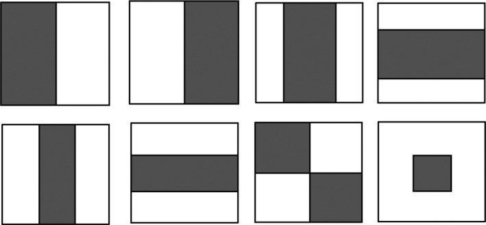
The standard Haar‐like features.

2.B.6. CT value histogram (CThist)

CT value histogram means the histogram of the CT values, which is the statistic probabilistic distribution of each density value in a CT image and is invariant in scale, rotation, and translation. In CT images, the CT values of pixels are expressed in the Hounsfield value (HU). We compute the histogram of CT values over a 7 × 7 window centered at each pixel. The number of bins in the histogram is 40, because it obtained the best performance according to.³²

2.C. Population learning and patient‐specific learning

In the training stage, we use the populartion learning and patient‐specific learning to obtain population knowledge and part of the patient‐specific knowledge for a new patient, respectively, by using the Adaboost classifier. Then, we combine the two knowledges together to guide the prostate segmentation for a new patient.

2.C.1. AdaBoost classifier

AdaBoost³³ is one of the most popular methods in ensemble learning. It can combine several learning algorithms (“weak learners”) to improve the performance in a weighted sum.

Let ε _t be the classification error of t‐th weak classifier and ln() is the log function to the base e, after which the weight of t‐th weak classifier a _t can be computed by

$$a_t=\frac{1}{2}\text{ln}(\frac{1-{\mathit{\epsilon }}_t}{{\mathit{\epsilon }}_t}).$$ (5)

Let x be the test sample and T be the number of weak classifier, after which h _t (x) is the hypothesis of t‐th weak classifier. Therefore, Adaboost can construct a “strong” classifier as a linear combination by

$$f(x)={\sum }_{t=1}^T{a}_t{h}_t(x)$$ (6)

Then AdaBoost offers the final decision according to the sign of f(x), like

$$H(x)=sign(f(x))$$ (7)

AdaBoost can force the weak classifier to focus on the hard examples in the training set by increasing the weights of incorrectly classified examples and thus it can converge to a strong learner. Since a decision tree owns the fast speed and superior performance, usually it is chosen as the week classifier.³⁴ Thus, we adopt the AdaBoost with the decision tree as our learning method for a good classification performance.

2.C.2. Population knowledge and patient‐specific knowledge

For the population learning, we extract the six discriminant features of each pixel in the registered prostates from the training set. We use the Adaboost classifier to train the population model, represented by Ada_PO. For the patient‐specific learning, we need the user to provide part of the information from the new patient. The user provides the contours of the prostate on three slices, i.e., the base, mid‐gland, and apex slices. According to the feature of each pixel and its label on the three slices, we train three, patient‐specific models represented by Ada_PAB, Ada_PAM, and Ada_PAA.

2.D. Prostate‐likelihood prediction based on the population and patient‐specific knowledge

Because the prostates from different patients vary greatly in size, shape, and position in the CT images, it is not straightforward to apply prior population knowledge to a new patient data. The learned patient‐specific knowledge based on the base, mid‐gland, and apex slices may have the problem of overfitting. Therefore, we combine the patient‐specific knowledge with the general population statistics to achieve more accurate segmentation.

We compute the similarity between the population knowledge and patient‐specific knowledge as the useful knowledge to the new patient, which can be used to predict the probabilities of the pixels on the slices except the base, mid‐gland, and apex slice. Let P _PAB (i), P _PAM (i), and P _PAA (i) be the probability of the pixel i predicted by the models Ada_PAB, Ada_PAM, and Ada_PAA, respectively, and S(PO, PAB), S(PO, PAM), and S(PO, PAA) be the similarity between the population model and the patient‐specific models on the base, mid‐gland, and apex slices, respectively. The final probability of belonging to the prostate for the pixel i, P(i), is computed by

$$P(i)=S(PO,PAB)·P_{PAB}(i)+S(PO,PAM)·P_{PAM}(i)+S(PO,PAA)·P_{PAA}(i).$$ (8)

For the given model M1 and M2, we use D _M2 to present the pixel set used to train the model M2, N _M2 to present the maximum of the real number of pixels belonging to the prostate and the number of predicted prostate pixels by the model M2, L _M1(k), and True(k) to be the label predicted by the model M1 and the true label of pixel k, respectively. And use SIM(L, C) as a function measuring the similarity between the two labels:

$$SIM(L,C)=\left\{\begin{array}{cc}1,& ifC=Landtheyareprostate\\ 0,& others\end{array}\right..$$ (9)

Then we compute the similarity of the two models, M1 and M2, S(M1, M2), by

$$S(M1,M2)={\sum }_{k\in D_{M2}}\frac{SIM(L_{M1}(k),True(k))}{N_{M2}}.$$ (10)

In (8), we compute the accuracy of the population model on the base, mid‐gland, and apex slices, as the similarity between the population model and the base, mid‐gland, and apex models, respectively. The accuracy represents the consistency between the population and patient‐specific knowledge. And it also indicates a proportion of the general population knowledge which is applicable to a specific patient. Then, we multiply the probability obtained by the patient‐specific model by the similarity of the population and patient‐specific model, and use the product as the probability of the pixel belonging to the prostate. The product can address the influences of applicable knowledge to capture the patient‐specific characters more accurately and then improve the accuracy of computing the probability. We combine the probability obtained by the three, weighted, patient‐specific models into a sum to represent the final probability to improve the stability and accuracy.

2.E. Adaptively binary prostate segmentation based on the area distribution model

On the basis of the predicted probability belonging to the prostate, we develop an adaptive threshold selection method based on the area distribution model to produce the prostate segmentation. For each patient in the training set, we compute the area of the prostate, i.e., the sum of the number of pixels belonging to the prostate, on each slice to produce its area distribution. We then create the model of the prostate area distribution by averaging the area distribution of each training 3D prostate image. Let ADM and AD(T) be the area distribution model and the area distribution of the patient to be segmented with the threshold T, respectively, and BD(·) be a Bhattacharyya distance function measuring the similarity of two discrete or continuous probability distributions. Then the optical threshold T can be computed by

$$T^{}\ast =argminBD(ADM,AD(T)).$$ (11)

Let p, q be the discrete probability distributions over the same domain X and BC(p, q) is the Bhattacharyya coefficient, which is a measure of the amount of overlap between p and q. Then their Bhattacharyya distance is defined by

$$BD(p,q)=-\text{ln}(BC(p,q)).$$ (12)

And the Bhattacharyya coefficient, BC(p, q), can be calculated by

$$BC(p,q)={\sum }_{x\in X}\sqrt{p(x)·q(x)}.$$ (13)

On the basis of the optimal threshold value, we segment the probability image into the prostate and non‐prostate pixels. We then combine these 2D prostate masks to form a 3D segmented prostate. Finally, we use a Gaussian smoothing method to achieve a smoothed 3D segmented prostate.

2.F. Evaluation criterion

To evaluate the performance of the segmentation, the Dice similarity coefficient (DSC), sensitivity, specificity, detection, false negative rate (FNR) and overlap error (OVE) were investigated in our segmentation experiments.³⁵

DSC is the relative volume overlap ratio between the binary masks from our method and the gold standard established by the expert‐defined segmentation. Sensitivity and specificity are widely used in the medical image analysis and are essentially two measurements of performance. Sensitivity measures the proportion of actual positives which are correctly identified as the prostate. Specificity measures the proportion of negatives which are correctly identified as non‐prostate. Detection is the detection rate, which is defined as the number of true positive voxels divided by the sum of the number of the false positive voxels and the number of the false negative voxels. The false negative rate (FNR) and the overlap error (OVE) are the evaluation criterion of error detection. The FNR was defined as the number of false negative voxels divided by the total number of the prostate voxels on the gold standard and the overlap error (OVE) is the nonoverlap area between the segmented result and the gold standard.

3. Experimental results

3.A. Databases and gold standards

We collected 3D CT image volumes from 92 prostate patients who underwent PET/CT scans. All the collected prostate CT images are from a GE scanner, and the volumetric data were saved slice by slice in the DICOM format. The slice thickness is 4.25 mm, and the size of the images is 512 × 512 × 27 voxels. The prostate was manually segmented independently three times by each of two, clinically experienced radiologists to produce the gold standards, and any two manual segmentations by the same radiologist were performed at least 1 week apart to eliminate the interference of previous manual segmentation. We use G1, G2, and G3 to represent the three manual segmentations obtained by Radiologist 1. We use G4, G5, and G6 to represent the three manual segmentations obtained by Radiologist 2. To obtain a robust gold standard, we adopt majority voting to fuse the labels from six manual segmentations to obtain a fused gold standard, G7. In our experiment, we conducted five‐fold cross‐validation experiments of the prostate segmentation using the seven gold standards.

To assess the inter‐observer and intra‐observer variability, we use the DSC to evaluate the segmentation performance. Tables 1 and 2 show the intra‐observer variations of the prostate segmentation for Radiologist 1 and Radiologist 2, respectively. In Tables 1 and 2, the DSC values of three times are close, and thus indicating that the manual segmentations by the radiologists were robust. The inter‐observer variations are shown in Table 3. The DSC varies from 87.12% to 93.73%, indicating that the manual segmentation is reliable and sufficiently confident.

Table 1.

Intra‐observer variation in prostate segmentation for radiologist 1 for three times

DSC (%)	Radiologist 1, time 1	Radiologist 1, time 2	Radiologist 1, time 3
Radiologist 1, time 1	100.0	96.68	93.64
Radiologist 1, time 2	96.68	100.00	93.07
Radiologist 1, time 3	93.64	93.07	100.0

Table 2.

Intra‐observer variation in prostate segmentation for radiologist 2 for three times

DSC (%)	Radiologist 2, time 1	Radiologist 2, time 2	Radiologist 2, time 3
Radiologist 2, time 1	100.0	93.91	92.03
Radiologist 2, time 2	93.91	100.0	95.44
Radiologist 2, time 3	92.03	95.44	100.0

Table 3.

Inter‐observer variation in prostate segmentation for radiologists 1 and 2 for three times

DSC (%)	Radiologist 2, time 1	Radiologist 2, time 2	Radiologist 2, time 3
Radiologist 1, time 1	91.67	88.25	87.12
Radiologist 1, time 2	93.73	89.70	88.40
Radiologist 1, time 3	91.58	88.31	87.24

3.B. Parameter tuning

The only parameter of our approach is the number of decision trees (week classifier) in AdaBoost during the training procedure. As a too large a number leads to long running time, and a too small a number leads to a bad modeling, we conducted the five‐fold cross‐validation experiments in the training data to test seven numbers, including 10, 20, 30, 50, 100, 150, and 200, to achieve the optimal tradeoff between the running time and classification accuracy rate. For each tested number, N, we trained the AdaBoost with N decision trees on the training data with G7 as the gold standard and recorded the classification accuracy rate on the training data. The average results are shown in Fig. 6. The number of 100 was chosen and was used in all of the following experiments.

Figure 6.

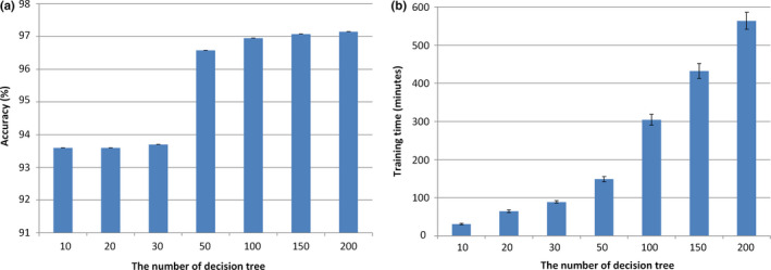
(a) Accuracy and (b) training time for different numbers of decision trees in AdaBoost. [Color figure can be viewed at wileyonlinelibrary.com]

3.C. The effectiveness of extracted features

To better character the prostate tissue, except for the intensity, we extracted five, different kinds of features, including mrLBP, HOG, GLCM, Haar like, and CThist. We conducted the five‐fold, cross‐validation experiments in the training data to test the distinguishing ability of features between prostate pixel and non‐prostate pixel. Since the number of non‐prostate pixels is far greater than that of prostate pixels, we computed the average sensitivity of the prostate for better measuring the ability to identify the prostate tissue. We show the results in Fig. 7 in which we can see that each feature can achieve more than 70% sensitivity and which proves that the features we chose are discriminant for our prostate segmentation problem. In addition, we linked these features together to obtain the combined features. Figure 7 showed that our combined features achieve the highest sensitivity and which proves that our combined features can provide the complementary information for better distinguishing between prostate pixel and non‐prostate pixel. Therefore, we can demonstrate that the extracted features are effective for prostate segmentation.

Figure 7.

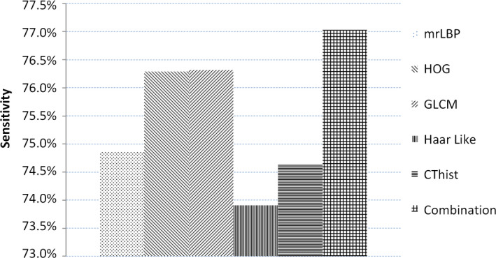
The sensitivity of each feature and combined features. [Color figure can be viewed at wileyonlinelibrary.com]

3.D. The effectiveness of adaptively binary prostate segmentation based on the area distribution model

To prove that our adaptive threshold obtained by the area distribution model can improve segmentation performance, first we show an example of one specific patient in Fig 8 in which we show the different thresholds, the different similarities of the area distribution model, and the area distributions obtained by different thresholds as well as the different DSC values obtained by different thresholds. We can see that we get 17 candidate thresholds, from −2 to 14. For each threshold, we can obtain a segmented prostate and its area distribution. Then, we compare its area distribution with the area distribution model and calculate their distance, as shown as the stippled bar in Fig. 8. Finally, to see the relationship between the threshold and segmentation performance, we compute the DSC between the segmented prostate with different thresholds and the gold standard, as shown as the striped bar. We find that the minimum distance corresponds to the best segmentation performance.

Figure 8.

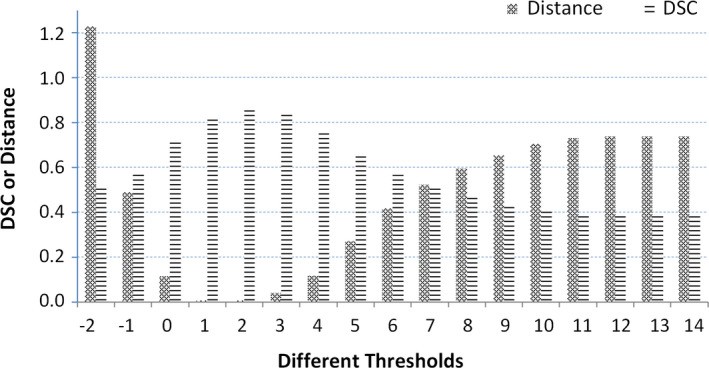
Different DSCs and distances between the area distribution model and area distributions obtained by different thresholds. [Color figure can be viewed at wileyonlinelibrary.com]

Second, we prove the advantage of our adaptive threshold selection by comparing the results with a fixed threshold (the threshold is fixed as zero). We conducted the experiments in the same way except the binary processing and show the results in Fig. 9. Our adaptive threshold selection can obtain a higher DSC and sensitivity as well as a lower false negative rate and overlap error. This proves that our adaptive threshold can improve segmentation performance.

Figure 9.

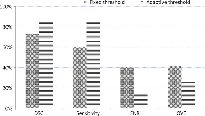
The average of the dice similarity coefficient, sensitivity, false negative rate, and overlap error from data from 92 patients for our adaptive threshold selection and the fixed threshold method. [Color figure can be viewed at wileyonlinelibrary.com]

3.E. The effectiveness of training three, patient‐specific models

In this study, we train three, patient‐specific models to learn the characteristics of a specific patient. We used the information on the base, mid‐gland, and apex slices to train three, patient‐specific models (3‐Model Method) for better charactering the test patient. To highlight the advantages of our three, patient‐specific models, we compared our method with the method that uses just one patient‐specific model (1‐Model Method). We used the information on the three slices to train one model rather than three models.

Similarly, let P _PA (i) be the probability of the pixel i predicted by the one patient‐specific model and S(PO, PA) be the similarity between the population model and the patient‐specific model, computed by (10). Therefore, the final probability of belonging to the prostate for the pixel i, P ¹(i), is computed by

$$P_{}^1(i)=S(PO,PA)·P_{PA}(i)$$ (14)

We then use the adaptive threshold method to obtain the best threshold. We compare the performance between the 3‐Model Method and the 1‐Model method and show the results in Fig. 10, which show that our 3‐Model method can achieve better performance because our method considers the particular characteristic of the prostate in the base, mid‐gland, and apex regions.

Figure 10.

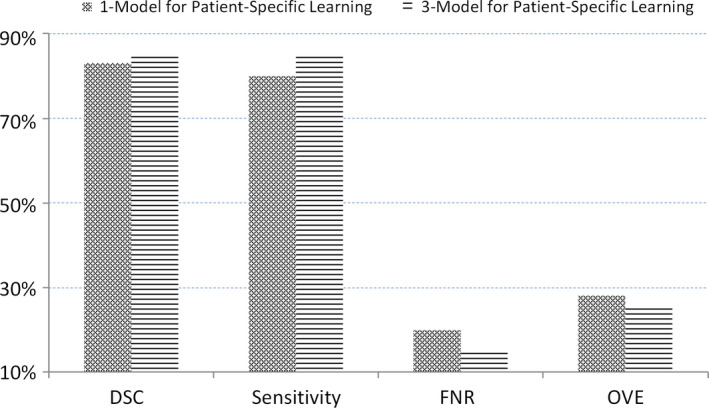
The average of dice similarity coefficient, sensitivity, false negative rate, and overlap error from 92 patients' data for our 3‐Model method and the 1‐Model method. [Color figure can be viewed at wileyonlinelibrary.com]

3.F. The segmentation performance of the fivefold cross‐validation

The segmented results for the 92 patients' data are shown in Table 4. Even for different manual segmentations as the gold standard, our approach achieved a maximum DSC of 87.18% and a minimal DSC of 83.58%, a maximum sensitivity of 87.46% and a minimal sensitivity of 83.28%, a maximum specificity of 97.94% and a minimal specificity of 97.34%, a maximum detection of 3.63 and a minimal detection of 2.86, a maximum false negative rate of 16.72% and a minimal false negative rate of 12.54%, and a maximum overlap error of 27.81% and a minimal overlap error of 22.61%. These results are close and our method achieved high segmentation performance no matter which manual segmentation was used as the gold standard, and thus indicating that our method is robust and effective.

Table 4.

The dice similarity coefficient, sensitivity, specificity, detection, false negative rate, and overlap error, of 92 CT images in the 5‐fold cross‐validation for different gold standards (G1‐G7), where the bold values denote the best results among the seven gold standards

	1	2	3	4	5	Average
DSC (%)
G1	86.78 ± 4.76	85.82 ± 4.10	86.69 ± 2.92	87.15 ± 2.85	85.73 ± 5.07	86.43 ± 3.98
G2	87.38 ± 3.13	86.53 ± 3.89	87.27 ± 2.86	87.10 ± 2.64	87.60 ± 2.51	87.18 ± 2.99
G3	87.11 ± 4.47	84.69 ± 5.64	86.96 ± 2.94	86.83 ± 3.06	87.04 ± 3.96	86.52 ± 4.14
G4	83.17 ± 6.35	84.08 ± 5.30	84.46 ± 4.12	86.21 ± 3.01	86.97 ± 3.63	84.98 ± 4.74
G5	81.15 ± 6.09	82.35 ± 5.84	83.97 ± 4.95	85.86 ± 4.01	84.55 ± 6.99	83.58 ± 5.77
G6	81.84 ± 4.95	82.06 ± 5.47	83.76 ± 4.67	85.73 ± 4.44	85.02 ± 6.30	83.68 ± 5.31
G7	84.79 ± 6.87	84.32 ± 4.36	83.80 ± 4.84	86.67 ± 3.05	85.58 ± 5.18	85.22 ± 4.99
SE (%)
G1	85.58 ± 8.49	84.51 ± 7.21	85.34 ± 5.02	91.54 ± 3.26	85.90 ± 9.49	86.58 ± 7.34
G2	86.65 ± 4.67	84.73 ± 6.56	86.85 ± 4.88	90.20 ± 4.21	88.87 ± 5.12	87.46 ± 5.37
G3	86.02 ± 8.84	82.38 ± 10.17	85.56 ± 5.76	88.65 ± 4.99	86.81 ± 7.88	85.88 ± 7.84
G4	81.35 ± 9.00	80.19 ± 9.48	84.6 ± 7.86	88.54 ± 5.08	86.44 ± 7.47	84.23 ± 8.33
G5	79.57 ± 7.73	79.81 ± 9.74	84.28 ± 8.40	88.39 ± 4.35	84.33 ± 10.26	83.28 ± 8.79
G6	81.22 ± 8.98	80.53 ± 9.93	84.45 ± 5.88	88.96 ± 5.76	84.54 ± 9.50	83.94 ± 8.55
G7	84.02 ± 10.94	80.66 ± 8.06	84.49 ± 7.58	88.96 ± 4.77	84.79 ± 10.45	84.91 ± 8.84
SP (%)
G1	97.69 ± 0.77	97.34 ± 1.51	97.82 ± 1.07	96.99 ± 0.86	97.37 ± 0.88	97.44 ± 1.07
G2	97.28 ± 2.05	97.65 ± 1.13	97.72 ± 0.94	97.21 ± 0.75	97.24 ± 1.29	97.42 ± 1.30
G3	97.98 ± 0.65	97.85 ± 1.10	98.12 ± 0.89	97.66 ± 0.68	97.89 ± 0.82	97.90 ± 0.84
G4	97.49 ± 1.22	98.17 ± 0.80	97.56 ± 0.83	97.53 ± 0.79	97.89 ± 0.84	97.73 ± 0.92
G5	97.19 ± 1.10	97.67 ± 1.08	97.52 ± 0.90	97.42 ± 1.16	97.45 ± 1.21	97.45 ± 1.08
G6	97.10 ± 1.18	97.42 ± 1.03	97.32 ± 1.02	97.36 ± 1.28	97.52 ± 0.90	97.34 ± 1.07
G7	97.86 ± 0.92	98.36 ± 0.84	97.60 ± 1.07	97.84 ± 0.55	98.05 ± 0.90	97.94 ± 0.89
DET
G1	3.63 ± 1.14	3.42 ± 1.64	3.43 ± 0.88	3.58 ± 0.95	3.34 ± 1.06	3.48 ± 1.14
G2	3.68 ± 0.98	3.66 ± 1.82	3.60 ± 0.86	3.54 ± 0.85	3.67 ± 0.75	3.63 ± 1.10
G3	3.73 ± 1.20	3.30 ± 1.78	3.50 ± 0.80	3.47 ± 0.81	3.63 ± 1.00	3.53 ± 1.16
G4	2.87 ± 1.19	3.10 ± 1.62	2.93 ± 0.88	3.29 ± 0.82	3.61 ± 1.10	3.16 ± 1.16
G5	2.43 ± 0.95	2.75 ± 1.52	2.92 ± 1.09	3.26 ± 0.89	3.24 ± 1.29	2.92 ± 1.18
G6	2.48 ± 0.96	2.51 ± 0.80	2.80 ± 0.86	3.28 ± 1.02	3.24 ± 1.14	2.86 ± 1.00
G7	3.24 ± 1.18	3.03 ± 1.45	2.80 ± 0.80	3.42 ± 0.81	3.30 ± 1.08	3.18 ± 1.09
FNS (%)
G1	14.42 ± 8.49	15.49 ± 7.21	14.63 ± 5.02	8.46 ± 3.26	14.10 ± 9.49	13.42 ± 7.34
G2	13.35 ± 4.67	15.27 ± 6.56	13.15 ± 4.88	9.80 ± 4.21	11.13 ± 5.12	12.54 ± 5.37
G3	13.98 ± 8.84	17.62 ± 10.17	14.44 ± 5.76	11.35 ± 4.99	13.19 ± 7.88	14.12 ± 7.84
G4	18.65 ± 9.00	19.81 ± 9.48	15.4 ± 7.86	11.46 ± 5.08	13.56 ± 7.47	15.78 ± 8.33
G5	20.43 ± 7.73	20.19 ± 9.74	15.72 ± 8.40	11.61 ± 4.35	15.67 ± 10.26	16.72 ± 8.79
G6	18.78 ± 8.98	19.47 ± 9.93	15.55 ± 5.88	11.04 ± 5.76	15.46 ± 9.50	16.06 ± 8.55
G7	15.98 ± 10.94	19.34 ± 8.06	15.51 ± 7.58	11.04 ± 4.77	15.21 ± 10.45	15.09 ± 8.84
OVE (%)
G1	23.09 ± 6.93	24.63 ± 6.33	23.39 ± 4.52	22.67 ± 4.47	24.66 ± 7.36	23.69 ± 5.95
G2	22.29 ± 4.86	23.54 ± 6.14	22.48 ± 4.40	22.76 ± 4.15	21.98 ± 3.88	22.61 ± 4.66
G3	22.59 ± 6.61	26.17 ± 8.41	22.97 ± 4.51	23.16 ± 4.67	22.76 ± 5.92	23.53 ± 6.18
G4	28.34 ± 9.06	27.12 ± 7.98	26.69 ± 6.11	24.12 ± 4.63	22.89 ± 5.60	25.83 ± 6.99
G5	31.32 ± 8.47	29.61 ± 8.50	27.34 ± 7.29	24.59 ± 5.90	26.20 ± 9.82	27.81 ± 8.26
G6	30.46 ± 7.09	30.09 ± 7.58	27.69 ± 6.75	24.74 ± 6.47	25.61 ± 8.76	27.72 ± 7.55
G7	25.88 ± 9.44	26.87 ± 6.61	27.62 ± 6.80	23.41 ± 4.65	24.90 ± 7.43	25.49 ± 7.13

3.G. The visualization of the segmented prostate

We randomly chose the slices except for the base, apex, and mid‐gland slices from different patients. We applied our segmented method to obtain the boundary of the prostate on these slices. Figure 11 shows that our segmented boundary accurately matches the manual segmentation.

Figure 11.

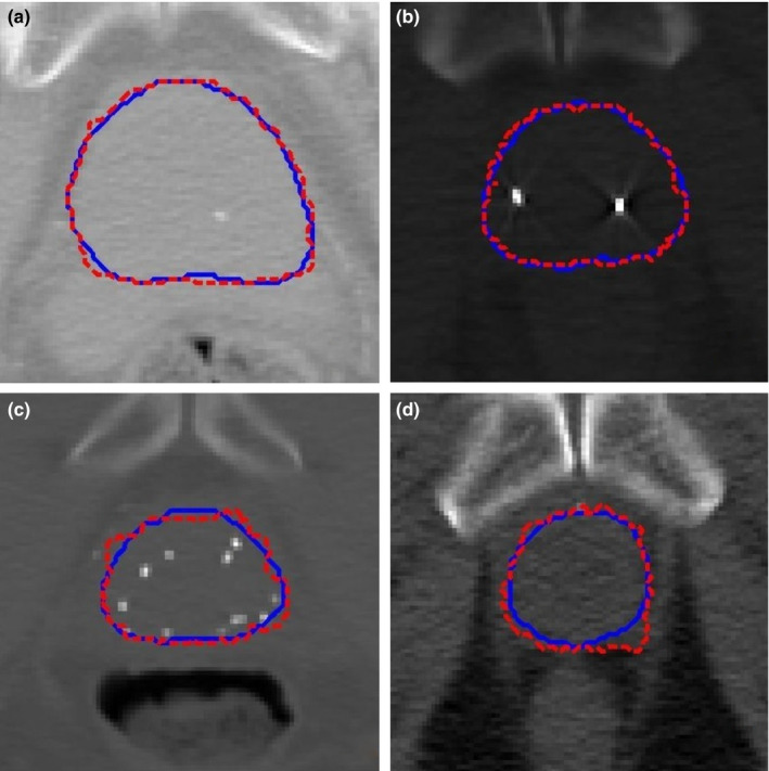
The segmented prostate on 2D slices (a)–(d) where the dash red boundaries were obtained by our method and the solid blue boundaries were obtained by manual segmentation. [Color figure can be viewed at wileyonlinelibrary.com]

3.H. Comparison with the pure population learning and pure patient‐specific learning methods

To illustrate the effectiveness of our combined method, we compare it with the pure population learning method (POL) and the pure patient‐specific learning method (PSL). The POL trains the model based only on the population data, whereas PSL is based only on the part of the new patient data. They use their trained models to identify the class (prostate or non‐prostate) of pixels to complete the prostate segmentation. In our experiments, we use the same classifier and still conduct the fivefold cross‐validation experiments to segment the prostate for the 92 patients by using POL, PSL, and our method POPSL. The comparison results are shown in Fig. 12. The DSC from our method is highest among the three methods, and the overlap error is the lowest. Our method achieved the highest performance compared with the other two, pure learning methods. It demonstrates that our method can take advantage of each pure leaning method and overcome the weaknesses of each learning method by combining the population and patient‐specific characteristics.

Figure 12.

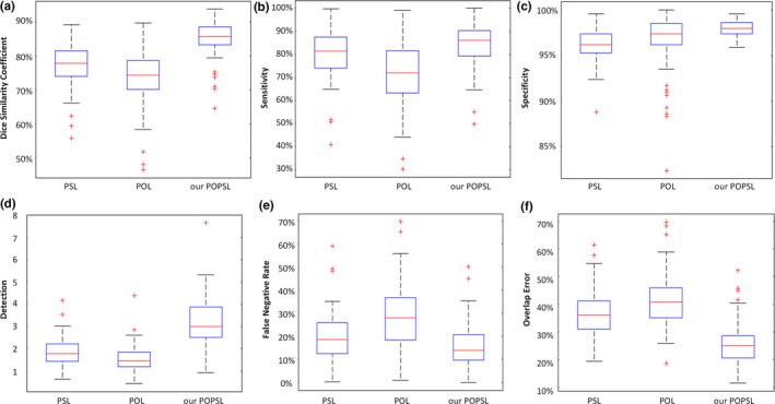
(a) The dice similarity coefficient, (b) sensitivity, (c) specificity, (d) detection, (e) false negative rate, and (f) overlap error for the 92 patient data by using the pure population learning method (POL), the pure patient‐specific learning method (PSL), and our method (POPSL). [Color figure can be viewed at wileyonlinelibrary.com]

3.I. Comparison with the other prostate segmentation methods

Our method is part of the method combining the population learning and patient‐specific learning together. To prove the effectiveness of our method, we compare our method with the other combination method.^{24, 25} Compared with the method²⁴ which conducted the prostate segmentation on 30 CT images, method²⁵ used 32 patients, and our database contains 92 patients. We also list the different collection schemes of the compared methods and our method in the last column in Table 5. Different from the method²⁴ iteratively getting the patient‐specific information, we access the information once. Different from method,²⁵ we do not need the planning and treatment images. Our DSC is greater or equal to the one in method²⁴ and the one in method²⁵ when they used planning image information. Therefore, we recognize that our method is effective compared with the other methods.

Table 5.

Comparison with the other prostate ct segmentation methods

Method	Database	DSC	Collection of patient‐specific information
Method24	30 CT images	0.865–0.872	Manual annotation iteratively
Method25	32 patients with 478 images	0.89	Manual annotation in one planning image and four treatment images
		0.85	Manual annotation in a planning CT
Ours	92 patients with 92 CT images	0.872	Manual annotation on three slices

3.J. The robustness of our method

Finally, we test the sensitivity of our method to the selection of the apex, middle, and base slices. Our method requires the user to select three slices to obtain the patient‐specific information for guiding the segmentation. To evaluate the effect of selecting the three slices, we perform our segmentation method on the neighboring slices around the apex, middle, and base slices. If S(A), S(M), and S(B) are the selected slices at the apex, mid‐gland, and base, respectively, then the neighboring slices are S(A + 1), S(A‐1), S(M + 1), S(M‐1), S(B + 1), and S(B‐1). We randomly choose five patients and use the neighboring slices to test the segmentation individually and jointly. We show the evaluation results in Fig. 13 in which the standard deviations of the five patients are very small. This proves that our method is robust regarding the selection of apex, middle, and base slices.

Figure 13.

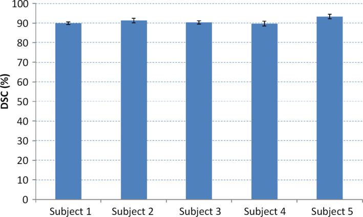
The effect of selecting three, key slices on the segmentation performance for five, random patients. [Color figure can be viewed at wileyonlinelibrary.com]

4. Discussion

We proposed and evaluated a learning‐based segmentation algorithm for the prostate in 3D CT images. The method combines the population and patient‐specific learning methods to improve the segmentation performance. The main contributions of this manuscript include (a) the combination of population and patient‐specific knowledge, (b) the adaptive selection of the threshold value for binarization, and (c) the robustness of our segmentation method.

We used the data from the other patients to obtain the general knowledge and used partial data from the new patient to obtain the specific knowledge. We combined them together to achieve the applicable population and patient‐specific knowledge. Because the prostates from different patients may have different size or shape and because of the inter‐patient variations, some population knowledge may not be applicable to a new patient. For the apex region, the mid‐gland region and the base region, we choose three slices of the new patient to train three, patient‐specific models for a better description of the prostate of the new patient. The combined population and patient‐specific knowledge can maximize the useful knowledge and minimize contradictory knowledge for a specific patient to improve the segmentation performance. The experimental results show that our combined method outperforms any single, learning‐based method alone. Our method is robust to the user interaction and the training data. Our method can compute the likelihood of each pixel in the CT image belonging to the prostate region more accurately. Hence, compared with the other combined learning methods, our method is effective and robust.

After obtaining the prostate likelihood for each pixel of the new patient image using the combined learning, we did not use a fixed threshold value to obtain the prostate or non‐prostate pixels. We calculated an adaptive value which was closely related to the specific patient to binary the prostate or non‐prostate pixels. We considered both the general shape of the prostate and the specific prostate likelihood to obtain a case‐specific value for a good performance. As shown in the experimental results, the calculated adaptive threshold value can achieve higher segmentation performance compared with the other values.

To evaluate the robustness of the selection of the slices, we recorded the slice numbers of the apex slice, middle slice, and base slice from the gold standards and we found that there is up to ±1 slice difference between every two gold standards. We performed our segmentation method using the ± neighboring slices and also achieved satisfactory DSC values. It indicates that our method is robust to the user selection of the slices.

The proposed method was implemented in MATLAB codes. The algorithm takes approximately 11.31 s to segment one prostate volume in 3D CT images in a Windows 7 desktop with a 32 GB RAM and 3.40 GHz processor. It contains approximately 10.95 s for recognition, 0.18 s for binarization, and 0.18 s for smoothing. Our code is not optimized and does not use multi‐thread, GPU acceleration or parallel programming. The segmentation method can be further speeded up for many applications in the management of prostate cancer patients.

5. Conclusion

We propose a learning‐based segmentation scheme that combines the population learning and patient‐specific learning together for segmenting the prostate on 3D CT images. The method overcomes the inter‐patient variations by taking advantage of the patient‐specific learning. It also takes advantage of the population learning to improve the segmentation performance. We use an adaptive threshold method to improve segmentation accuracy. Experimental results demonstrate the effectiveness and robustness of the method. The learning‐based segmentation method can be applied to prostate imaging applications, including targeted biopsy, diagnosis, and treatment planning of the prostate.

References

- 1. Siegel RL, Miller KD, Jemal A. Cancer statistics, 2016. CA Cancer J Clin. 2015;66:7–30. [DOI] [PubMed] [Google Scholar]
- 2. Ghose S, Oliver A, Marti R, et al. A survey of prostate segmentation methodologies in ultrasound, magnetic resonance and computed tomography images. Comput Meth Programs Biomed. 2012;108:262–287. [DOI] [PubMed] [Google Scholar]
- 3. Acosta O, Dowling J, Cazoulat G, et al. Atlas based segmentation and mapping of organs at risk from planning CT for the development of voxel‐wise predictive models of toxicity in prostate radiotherapy. In: Madabhushi A, Dowling J, Yan P, Fenster A, Abolmaesumi P, Hata N, eds. International Workshop on Prostate Cancer Imaging. Berlin: Springer; 2010:42–51. [Google Scholar]
- 4. Acosta O, Simon A, Monge F, et al. Evaluation of multi‐atlas‐based segmentation of CT scans in prostate cancer radiotherapy. In: Wright S, ed. 2011 IEEE International Symposium on Biomedical Imaging: From Nano to Macro. Chicago, IL: IEEE; 2011:1966–1969. [Google Scholar]
- 5. Bueno G, Deniz O, Salido J, Carrascosa C, Delgado JM. A geodesic deformable model for automatic segmentation of image sequences applied to radiation therapy. Int J Comput Assist Radiol Surg. 2011;6:341–350. [DOI] [PubMed] [Google Scholar]
- 6. Chai X, Xing L. SU‐E‐J‐92: multi‐atlas based prostate segmentation guided by partial active shape model for CT image with gold markers. Med Phys. 2013;40:171–171. [Google Scholar]
- 7. Chen S, Radke RJ. Level set segmentation with both shape and intensity priors. In: Matsuyama T, ed. 2009 IEEE 12th International Conference on Computer Vision. Kyoto: IEEE; 2009:763–770. [Google Scholar]
- 8. Chen T, Kim S, Zhou J, Metaxas D, Rajagopal G, Yue N. 3D meshless prostate segmentation and registration in image guided radiotherapy. Med Image Comput Comput Assist Interv. 2009;2009:43–50. [DOI] [PubMed] [Google Scholar]
- 9. Cosio FA, Flores JAM, Castaneda MAP. Use of simplex search in active shape models for improved boundary segmentation. Pattern Recognit Lett. 2010;31:806–817. [Google Scholar]
- 10. Costa MJ, Delingette H, Novellas S, Ayache N. Automatic segmentation of bladder and prostate using coupled 3D deformable models. Med Image Comput Comput Assist Interv. 2007;2007:252–260. [DOI] [PubMed] [Google Scholar]
- 11. Ghosh P, Mitchell M. Prostate segmentation on pelvic CT images using a genetic algorithm. In: Reinhardt JM, Pluim JPW, eds. Medical Imaging, International Society for Optics and Photonics. San Diego, CA: SPIE; 2008:691442–691442. [Google Scholar]
- 12. Rousson M, Khamene A, Diallo M, Celi JC, Sauer F. Constrained surface evolutions for prostate and bladder segmentation in CT images. In: Liu Y, Jiang T, Zhang C, eds. International Workshop on Computer Vision for Biomedical Image Applications. Berlin: Springer; 2005:251–260. [Google Scholar]
- 13. Tang X, Jeong Y, Radke RJ, Chen GT. Geometric‐model‐based segmentation of the prostate and surrounding structures for image‐guided radiotherapy. In: Panchanathan S, Vasudev B, eds. Electronic Imaging, International Society for Optics and Photonics. San Jose, CA: SPIE; 2004:168–176. [Google Scholar]
- 14. Wu Y, Liu G, Huang M, et al. Prostate segmentation based on variant scale patch and local independent projection. IEEE Trans Med Imaging. 2014;33:1290–1303. [DOI] [PubMed] [Google Scholar]
- 15. Shi Y, Liao S, Gao Y, Zhang D, Gao Y, Shen D. Transductive prostate segmentation for CT image guided radiotherapy. In: Wang F, Shen D, Yan P, Suzuki K, eds. International Workshop on Machine Learning in Medical Imaging. Berlin: Springer; 2012:1–9. [Google Scholar]
- 16. Shi Y, Liao S, Gao Y, Zhang D, Gao Y, Shen D. Prostate segmentation in CT images via spatial‐constrained transductive lasso. In: Medioni G, Zabih R, eds. Proceedings of the IEEE Conference on Computer Vision and Pattern Recognition. Portland, OR: IEEE; 2013:2227–2234. [DOI] [PMC free article] [PubMed] [Google Scholar]
- 17. Liao S, Gao Y, Lian J, Shen D. Sparse patch‐based label propagation for accurate prostate localization in CT images. IEEE Trans Med Imaging. 2013;32:419–434. [DOI] [PMC free article] [PubMed] [Google Scholar]
- 18. Li W, Liao S, Feng QJ, Chen WF, Shen DG. Learning image context for segmentation of the prostate in CT‐guided radiotherapy. Phys Med Biol. 2012;57:1283–1308. [DOI] [PMC free article] [PubMed] [Google Scholar]
- 19. Gao YZ, Liao S, Shen DG. Prostate segmentation by sparse representation based classification. Med Phys. 2012;39:6372–6387. [DOI] [PMC free article] [PubMed] [Google Scholar]
- 20. Martínez F, Romero E, Dréan G, et al. Segmentation of pelvic structures for planning CT using a geometrical shape model tuned by a multi‐scale edge detector. Phys Med Biol. 2014;59:1471. [DOI] [PMC free article] [PubMed] [Google Scholar]
- 21. Gao Y, Wang L, Shao Y, Shen D. Learning distance transform for boundary detection and deformable segmentation in CT prostate images. In: Wu G, Zhang D, Zhou L, eds. International Workshop on Machine Learning in Medical Imaging. Cham: Springer; 2014:93–100. [DOI] [PMC free article] [PubMed] [Google Scholar]
- 22. Chen S, Lovelock DM, Radke RJ. Segmenting the prostate and rectum in CT imagery using anatomical constraints. Med Image Anal. 2011;15:1–11. [DOI] [PubMed] [Google Scholar]
- 23. Song Q, Liu YX, Liu YL, Saha PK, Sonka M, Wu XD. Graph search with appearance and shape information for 3‐D prostate and bladder segmentation. In: Jiang T, Navab N, Pluim JPW, Viergever MA, eds. International Conference on Medical Image Computing and Computer‐Assisted Intervention. Berlin: Springer; 2010:172–180. [DOI] [PubMed] [Google Scholar]
- 24. Park SH, Gao Y, Shi Y, Shen D. Interactive prostate segmentation using atlas‐guided semi‐supervised learning and adaptive feature selection. Med Phys. 2014;41:111715. [DOI] [PMC free article] [PubMed] [Google Scholar]
- 25. Gao Y, Zhan Y, Shen D. Incremental learning with selective memory (ILSM): towards fast prostate localization for image guided radiotherapy. IEEE Trans Med Imaging. 2014;33:518–534. [DOI] [PMC free article] [PubMed] [Google Scholar]
- 26. Liao S, Shen D. A feature‐based learning framework for accurate prostate localization in CT images. IEEE Trans Image Process. 2012;21:3546–3559. [DOI] [PubMed] [Google Scholar]
- 27. Ma L, Guo R, Tian Z, et al. Combining population and patient‐specific characteristics for prostate segmentation on 3D CT images. In: Styner MA, Angelini ED, eds. SPIE Medical Imaging, International Society for Optics and Photonics. San Diego, CA: SPIE; 2016:978427–978427. [DOI] [PMC free article] [PubMed] [Google Scholar]
- 28. Ojala T, Pietikäinen M, Harwood D. A comparative study of texture measures with classification based on featured distributions. Pattern Recogn. 1996;29:51–59. [Google Scholar]
- 29. Haralick RM, Shanmugam RM, Dinstein IH. Textural features for image classification. IEEE Trans Syst Man Cybern. 1973;6:610–621. [Google Scholar]
- 30. Dalal N, Triggs B. Histograms of oriented gradients for human detection. In: Schmid C, Soatto S, Tomasi C, eds. 2005 IEEE Computer Society Conference on Computer Vision and Pattern Recognition. San Diego, CA: IEEE; 2005:886–893. [Google Scholar]
- 31. Viola P, Jones M. Rapid object detection using a boosted cascade of simple features. In: Jacobs A, Baldwin T, eds. IEEE Computer Society Conference on Computer Vision and Pattern Recognition. Kauai, HI: IEEE; 2001:I–511. [Google Scholar]
- 32. Liu X, Ma L, Song L, Zhao Y, Zhao X, Zhou C. Recognizing common CT imaging signs of lung diseases through a new feature selection method based on Fisher criterion and genetic optimization. IEEE J Biomed Health Inform. 2015;19:635–647. [DOI] [PubMed] [Google Scholar]
- 33. Freund Y, Schapire RE. Experiments with a new boosting algorithm. Int Conf Mach Learn. 1996;96:148–156. [Google Scholar]
- 34. Safavian SR, Landgrebe D. A survey of decision tree classifier methodology. IEEE Trans Syst Man Cybern. 1990;21:660–674. [Google Scholar]
- 35. Fei B, Yang X, Nye JA, et al. MR/PET quantification tools: registration, segmentation, classification, and MR‐based attenuation correction. Med Phys. 2012;39:6443–6454. [DOI] [PMC free article] [PubMed] [Google Scholar]