Dosimetric characterization of the $\mathrm{M}-15$ high‐dose‐rate $\text{Iridium}-192$ brachytherapy source using the AAPM and ESTRO formalism

Abstract

The Source Production & Equipment Co. (SPEC) model $\mathrm{M}-15$ is a new $\text{Iridium}-192$ brachytherapy source model intended for use as a temporary high‐dose‐rate (HDR) brachytherapy source for the Nucletron microSelectron Classic afterloading system. The purpose of this study is to characterize this HDR source for clinical application by obtaining a complete set of Monte Carlo calculated dosimetric parameters for the M‐15, as recommended by AAPM and ESTRO, for isotopes with average energies greater than 50 keV. This was accomplished by using the MCNP6 Monte Carlo code to simulate the resulting source dosimetry at various points within a pseudoinfinite water phantom. These dosimetric values next were converted into the AAPM and ESTRO dosimetry parameters and the respective statistical uncertainty in each parameter also calculated and presented. The $\mathrm{M}-15$ source was modeled in an MCNP6 Monte Carlo environment using the physical source specifications provided by the manufacturer. $\text{Iridium}-192$ photons were uniformly generated inside the iridium core of the model $\mathrm{M}-15$ with photon and secondary electron transport replicated using photoatomic cross‐sectional tables supplied with MCNP6. Simulations were performed for both water and air/vacuum computer models with a total of $4\times {10}^9$ sources photon history for each simulation and the in‐air photon spectrum filtered to remove low‐energy photons below $\delta =10\mathrm{\%}\text{keV}$. Dosimetric data, including $\mathrm{D}(\mathrm{r},\theta ),{\mathrm{g}}_{\mathrm{L}}(\mathrm{r}),\mathrm{F}(\mathrm{r},\theta ),{\mathrm{\Phi }}_{\text{an}}(\mathrm{r})$, and ${\overline{\phi }}_{\text{an}}$, and their statistical uncertainty were calculated from the output of an MCNP model consisting of an $\mathrm{M}-15$ source placed at the center of a spherical water phantom of 100 cm diameter. The air kerma strength in free space, ${\mathrm{S}}_{\mathrm{K}}$, and dose rate constant, Λ, also was computed from a MCNP model with $\mathrm{M}-15$ $\text{Iridium}-192$ source, was centered at the origin of an evacuated phantom in which a critical volume containing air at STP was added 100 cm from the source center. The reference dose rate, $\dot{\mathrm{D}}({\mathrm{r}}_0,{\theta }_0)\equiv \dot{\mathrm{D}}(1\text{cm},\pi /2)$, is found to be $4.038\pm 0.064\hspace{0.17em}\text{cGy}\hspace{0.17em}{\text{mCi}}^{-1}\hspace{0.17em}{\mathrm{h}}^{-1}$. The air kerma strength, ${\mathrm{S}}_{\mathrm{K}}$, is reported to be $3.632\pm 0.086\hspace{0.17em}\text{cGy}\hspace{0.17em}{\text{cm}}^2\hspace{0.17em}{\text{mCi}}^{-1}\hspace{0.17em}{\mathrm{g}}^{-1}$, and the dose rate constant, Λ, is calculated to be $1.112\pm 0.029\hspace{0.17em}\text{cGy}\hspace{0.17em}{\mathrm{h}}^{-1}\hspace{0.17em}{\mathrm{U}}^{-1}$. The normalized dose rate, radial dose function, and anisotropy function with their uncertainties were computed and are represented in both tabular and graphical format in the report. A dosimetric study was performed of the new $\mathrm{M}-15$ $\text{Iridium}-192$ HDR brachytherapy source using the MCNP6 radiation transport code. Dosimetric parameters, including the dose‐rate constant, radial dose function, and anisotropy function, were calculated in accordance with the updated AAPM and ESTRO dosimetric parameters for brachytherapy sources of average energy greater than 50 keV. These data therefore may be applied toward the development of a treatment planning program and for clinical use of the source.

PACS numbers: 87.56.bg, 87.53.Jw

I. INTRODUCTION

$\text{Iridium}-192$ is a standard high‐dose‐rate brachytherapy isotope that has been well studied and tested for clinical treatments of lung, esophageal, prostate, cervical, coronary, and other diseases. ¹ , ² , ³ , ⁴ , ⁵ Source Production & Equipment Co. (SPEC) has developed a new $\text{Iridium}-192$ high‐dose‐rate brachytherapy source model, the M‐15, for use in temporary high‐dose‐rate (HDR) brachytherapy. This model was designed to be an alternative replacement source for the Nucletron microSelectron Classic HDR afterloading system, since Nucletron no longer manufactures replacement sources for that system.

In accordance with the recommendation of the AAPM and ESTRO for brachytherapy sources with average energies greater than 50 keV ⁽⁶⁾ and in accordance with the updated AAPM Task Group Report No. 43 (TG‐43U1), ⁽⁷⁾ this report performed a complete series of Monte Carlo simulations to obtain the dosimetric parameters of the model $\mathrm{M}-15$ $\text{Iridium}-192$ brachytherapy source. This was achieved using the MCNP6 Monte Carlo code ⁽⁸⁾ to obtain dosimetric data in both water and air/vacuum modeled environments; the resulting data used to calculate source dosimetric parameters at one‐degree increments from 0° to 10° and 170° to 180° and five‐degree increments from 10° to 170°, as recommended by AAPM and ESTRO. ⁽⁶⁾ The statistical uncertainties in each parameter also were calculated using the methods derived by Medich et al. ⁽⁹⁾ and are presented herein.

II. MATERIALS AND METHODS

A. Brachytherapy source geometry and composition

The methods employed in this investigation of the SPEC model $\mathrm{M}-15$ source were similar to the methods used previously for the SPEC model M‐19 $\text{Iridium}-192$ source. ⁽¹⁰⁾ To summarize, the $\mathrm{M}-15$ source was modeled in an MCNP Monte Carlo environment using the physical source specifications provided by the manufacturer. In this case, the MCNP6 code was used to obtain these results. A graphical depiction of the $\mathrm{M}-15$ schematic used in the Monte Carlo simulation is presented in Fig. 1, with its corresponding physical parameters listed in Table 1. The source construction was symmetric about the coaxial axis, but nonsymmetric about the traverse plane due to the addition of an attached source cable.

Figure 1.

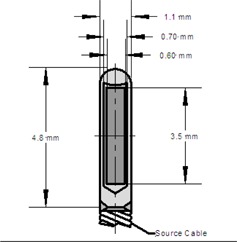
Configuration of the $\mathrm{M}-15$ $\text{Iridium}-192$ HDR brachytherapy source modeled for the MCNP simulation. This model consists of a 3.5 mm long $\text{Iridium}-192$ source encapsulated in a steel shell.

Table 1.

Physical parameters of the $\mathrm{M}-15$ $\text{Iridium}-192$ source used in the MCNP simulations.

Component	Outside Diameter (mm)	Inside Diameter (mm)	Length (mm)	Density (mg/mm3)	Remarks
Active	0.6	N.A	3.5	22.4	Iridium Metal
Encapsulation	1.1	0.7	4.8	7.8	Stainless Steel
Source Cable	1.1	N.A	2000	7.8	Stainless Steel

B. Monte Carlo calculation techniques

Radiation transport calculations were performed on a Windows‐based (Microsoft, Redmond, WA) personal computer running the MCNP6 Monte Carlo computer code. ⁽⁸⁾ $\text{Iridium}-192$ photons were uniformly generated inside the iridium core of the model $\mathrm{M}-15$ with photon and secondary electron transport replicated using default MCPLIB04 photoatomic cross‐sectional tables supplied with MCNP6. Simulations were performed for both water and air/vacuum computer models with a total of $4\times {10}^9$ sources photon history for each simulation. All simulations were performed in the photon and electron transport mode (Mode: p,e in the MCNP code) so that both primary photons and resulting secondary electrons were properly transported. ⁽¹¹⁾ The complete $\text{Iridium}-192$ photon spectrum, presented by Firestone and Ekström, ⁽¹²⁾ was used in these calculations and the total uncertainty in the spectrum, ${\sigma }_{\mathrm{I}\gamma }^{\text{relative}}=0.5\mathrm{\%}$, calculated as an intensity‐weighted average of the uncertainty in each spectral line also presented by Firestone and Ekström.

Dosimetric data, including $\dot{\mathrm{D}}(\mathrm{r},\theta ),{\mathrm{g}}_{\mathrm{L}}(\mathrm{r}),\mathrm{F}(\mathrm{r},\theta ),{\mathrm{\theta }}_{\text{an}}(\mathrm{r})$, and ${\overline{\phi }}_{\text{an}}$, and their statistical uncertainty(⁹) were calculated from the output of an MCNP computer model consisting of an $\mathrm{M}-15$ source placed at the center of a spherical water phantom of 100 cm diameter; this diameter was chosen to approximate an infinite water phantom, allowing for full photon scattering conditions in the dosimetric regions of interest. ¹¹ , ¹³ Dosimetric data were calculated at radial distances ranging from 0.5 to 15 cm in half centimeter increments and over angles ranging from 0° to 180°, using the MCNP6 F6 energy deposition tally, ${\mathrm{R}}_{\text{tally}}(\mathrm{r},\theta )$, reported in units of $\text{MeV}\hspace{0.17em}{\mathrm{g}}^{-1}\hspace{0.17em}{\text{photon}}^{-1}$.

The energy deposition tally output, ${\mathrm{R}}_{\text{tally}}$($\mathrm{r},\theta$), was multiplied by the $\text{Iridium}-192$ photon yield, ${\mathrm{I}}_{\gamma }=2.301\hspace{0.17em}\gamma \hspace{0.17em}{\text{Bq}}^{-1}\hspace{0.17em}{\mathrm{s}}^{-1}$, to obtain the calculated dose deposited in the tally region per disintegration, $\dot{\mathrm{D}}(\mathrm{r},\theta )$:

$$\dot{D}(r,\theta )=R_{MonteCarlo}(r,\theta )I_{\gamma }.$$ (1)

This result, expressed in units of $\text{MeV}\hspace{0.17em}{\mathrm{g}}^{-1}\hspace{0.17em}{\text{Bq}}^{-1}\hspace{0.17em}{\mathrm{s}}^{-1}$ was converted into more conventional units through the relationship: 1 $\text{MeV}\hspace{0.17em}{\mathrm{g}}^{-1}\hspace{0.17em}{\text{Bq}}^{-1}\hspace{0.17em}{\mathrm{s}}^{-1}=2.13\times 103\text{cGy}\hspace{0.17em}{\text{mCi}}^{-1}\hspace{0.17em}{\mathrm{h}}^{-1}$. ⁽¹⁰⁾

The air‐kerma strength in free space, ${\mathrm{S}}_{\mathrm{K}}$, was calculated using the methods described previously.⁽⁹) Briefly, the $\mathrm{M}-15$ $\text{Iridium}-192$ source was centered at the origin of an evacuated phantom in which a critical volume containing air at STP was added 100 cm from the source center. The MCNP6 *F4 tally $(\text{Mev}/{\text{cm}}^2)$ output from the air‐kerma simulation was multiplied by the respective air mass‐energy absorption coefficient, ${\mu }_{\text{en}}/p\hspace{0.17em}({\text{cm}}^2/\mathrm{g})$,⁽¹⁴) to obtain the air kerma per source photon $(\text{MeV}\hspace{0.17em}{\mathrm{g}}^{-1}\hspace{0.17em}{\text{photon}}^{-1})$. Equivalence is assumed between the air mass‐energy transfer coefficient and the air mass‐energy absorption coefficient due to negligible radiative energy losses. ⁽¹⁵⁾ The X‐ray cutoff energy, δ, was chosen to be $\delta =10\mathrm{\%}\text{keV}$;^(9,10) photons within the critical target with energies less than or equal to δ were removed from the final air‐kerma rate calculation. Once filtered, air‐kerma strength in free space is found by multiplying the square of the source to volume distance by the resulting air‐kerma rate.

III. RESULTS & DISCUSSION

A. Dose rate and normalized dose‐rate distribution

The Monte Carlo tally output ${\mathrm{R}}_{\text{tally}}$($\mathrm{r},\theta$) at each point of interest in the water phantom is converted to the dose rate $\dot{\mathrm{D}}(\mathrm{r},\theta )$ using Eq. (1). This dose rate corresponds to the updated AAPM TG‐43 dose rate in water:

$${\dot{D}}_{TG-43}(r,\theta )=S_K*\Lambda *\frac{G_L(r,\theta )}{G_L(r_0,{\theta }_0)}*g_L(r)*F(r,\theta )$$ (2)

The absolute uncertainty in $\dot{D}(r,\theta )$ was calculated as the quadrature sum of the relative simulation uncertainty, the relative uncertainty in the cross section tables, and the relative uncertainty in the photon yield, as presented in Eq. (3):

$${\sigma }_{\dot{D}}^{absolute}(r,\theta )=\sqrt{{({\sigma }_{MonteCarlo}^{relative}(r,\theta ))}^2+{({\sigma }_{cros\text{sec}tion}^{relative})}^2+{({\sigma }_{I_{{}^{\gamma }}}^{relative})}^2}$$ (3)

The data were next corrected for the geometry effect by multiplying the dose rate, $\dot{\mathrm{D}}(\mathrm{r},\theta )$, by the radial distance squared, r². The resulting dose rate is then normalized to the reference dose in water, $\dot{\mathrm{D}}({\mathrm{r}}_0,{\theta }_0)=4.038\pm 0.064\hspace{0.17em}{\text{cGy mCi}}^{-1}\hspace{0.17em}{\mathrm{h}}^{-1}$, to obtain ${\dot{\mathrm{D}}}_{\mathrm{N}}(\mathrm{r},\theta )$:

$${\dot{D}}_N(r,\theta )=\frac{\dot{D}(r,\theta )\cdot r^2}{\dot{D}(r_0,{\theta }_0)}$$ (4)

A graphical representation of the normalized dose rate is presented in Fig. 2. The tabular representation is also presented in Table 2, with the absolute uncertainty calculated using the equation:

$${\sigma }_{{\dot{D}}_N}^{absolute}(r,\theta )={\dot{D}}_N(r,\theta )\sqrt{{({\sigma }_{MonteCarlo}^{relative}(r,\theta ))}^2+{({\sigma }_{MonteCarlo}^{relative}(r_{0,}{\theta }_0))}^2+2{({\sigma }_{cross\text{sec}tion}^{relative})}^2}$$ (5)

Figure 2.

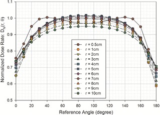
Presentation of the normalized dose‐rate distribution of model $\mathrm{M}-15$ $\text{Iridium}-192$ from the MCNP output. Geometry effects were removed by multiplying the dose rate, $\dot{\mathrm{D}}(\mathrm{r},\theta )$, by the radial distance squared, r². Once corrected, the dose rate is then normalized to the dose rate at 1 cm along the seed's traverse's axis, $\dot{\mathrm{D}}(\mathrm{r},\theta )=4.038\pm 0.064\hspace{0.17em}\text{cGy}\hspace{0.17em}{\text{mCi}}^{-1}\hspace{0.17em}{\mathrm{h}}^{-1}$, to obtain the normalized dose rate.

Table 2.

Calculated normalized dose rate distribution of the $\mathrm{M}-15$ $\text{Iridium}-192$ in water ${\dot{\mathrm{D}}}_{\mathrm{N}}(\mathrm{r},\theta )=[\dot{\mathrm{D}}(\mathrm{r},\theta )\cdot {\mathrm{r}}^2]\dot{\mathrm{D}}({\mathrm{r}}_0,{\theta }_0)$ with absolute uncertainty, ${\sigma }_{{\dot{\mathrm{D}}}_{\mathrm{N}}}$.

$r(cm)\theta \hspace{0.17em}(deg)$	0.5	1.0	2.0	3.0	4.0	5.0	6.0	7.0	8.0	9.0	10.0
0	$0.756\pm 0.016$	$0.650\pm 0.014$	$0.648\pm 0.014$	$0.674\pm 0.015$	$0.698\pm 0.015$	$0.716\pm 0.015$	$0.727\pm 0.016$	$0.736\pm 0.016$	$0.740\pm 0.016$	$0.740\pm 0.016$	$0.738\pm 0.016$
1	$0.760\pm 0.016$	$0.655\pm 0.014$	$0.654\pm 0.014$	$0.676\pm 0.014$	$0.698\pm 0.015$	$0.716\pm 0.015$	$0.730\pm 0.016$	$0.739\pm 0.016$	$0.744\pm 0.016$	$0.745\pm 0.016$	$0.742\pm 0.016$
2	$0.760\pm 0.016$	$0.656\pm 0.014$	$0.664\pm 0.014$	$0.688\pm 0.015$	$0.709\pm 0.015$	$0.725\pm 0.015$	$0.738\pm 0.016$	$0.747\pm 0.016$	$0.751\pm 0.016$	$0.752\pm 0.016$	$0.749\pm 0.016$
3	$0.761\pm 0.016$	$0.667\pm 0.014$	$0.677\pm 0.014$	$0.699\pm 0.015$	$0.720\pm 0.015$	$0.735\pm 0.016$	$0.747\pm 0.016$	$0.754\pm 0.016$	$0.758\pm 0.016$	$0.759\pm 0.016$	$0.755\pm 0.016$
4	$0.764\pm 0.016$	$0.681\pm 0.014$	$0.690\pm 0.015$	$0.712\pm 0.015$	$0.730\pm 0.015$	$0.745\pm 0.016$	$0.757\pm 0.016$	$0.764\pm 0.016$	$0.766\pm 0.016$	$0.765\pm 0.016$	$0.761\pm 0.016$
5	$0.775\pm 0.016$	$0.696\pm 0.015$	$0.703\pm 0.015$	$0.723\pm 0.015$	$0.741\pm 0.016$	$0.755\pm 0.016$	$0.765\pm 0.016$	$0.771\pm 0.016$	$0.773\pm 0.016$	$0.772\pm 0.016$	$0.767\pm 0.016$
6	$0.789\pm 0.017$	$0.710\pm 0.015$	$0.716\pm 0.015$	$0.734\pm 0.016$	$0.751\pm 0.016$	$0.764\pm 0.016$	$0.773\pm 0.016$	$0.779\pm 0.017$	$0.781\pm 0.017$	$0.778\pm 0.017$	$0.773\pm 0.016$
7	$0.803\pm 0.017$	$0.723\pm 0.015$	$0.727\pm 0.015$	$0.746\pm 0.016$	$0.761\pm 0.016$	$0.774\pm 0.016$	$0.782\pm 0.017$	$0.787\pm 0.017$	$0.787\pm 0.017$	$0.785\pm 0.017$	$0.779\pm 0.017$
8	$0.817\pm 0.017$	$0.736\pm 0.016$	$0.741\pm 0.016$	$0.758\pm 0.016$	$0.773\pm 0.016$	$0.785\pm 0.017$	$0.792\pm 0.017$	$0.796\pm 0.017$	$0.796\pm 0.017$	$0.793\pm 0.017$	$0.786\pm 0.017$
9	$0.830\pm 0.018$	$0.750\pm 0.016$	$0.753\pm 0.016$	$0.769\pm 0.016$	$0.783\pm 0.017$	$0.794\pm 0.017$	$0.801\pm 0.017$	$0.804\pm 0.017$	$0.804\pm 0.017$	$0.800\pm 0.017$	$0.792\pm 0.017$
10	$0.844\pm 0.018$	$0.764\pm 0.016$	$0.767\pm 0.016$	$0.782\pm 0.017$	$0.795\pm 0.017$	$0.805\pm 0.017$	$0.811\pm 0.017$	$0.813\pm 0.017$	$0.811\pm 0.017$	$0.807\pm 0.017$	$0.799\pm 0.017$
15	$0.906\pm 0.019$	$0.827\pm 0.018$	$0.825\pm 0.018$	$0.836\pm 0.018$	$0.845\pm 0.018$	$0.851\pm 0.018$	$0.853\pm 0.018$	$0.852\pm 0.018$	$0.847\pm 0.018$	$0.840\pm 0.018$	$0.829\pm 0.018$
20	$0.950\pm 0.020$	$0.875\pm 0.019$	$0.870\pm 0.018$	$0.878\pm 0.019$	$0.884\pm 0.019$	$0.887\pm 0.019$	$0.886\pm 0.019$	$0.883\pm 0.019$	$0.876\pm 0.019$	$0.866\pm 0.018$	$0.854\pm 0.018$
25	$0.978\pm 0.021$	$0.910\pm 0.019$	$0.904\pm 0.019$	$0.910\pm 0.019$	$0.914\pm 0.019$	$0.915\pm 0.019$	$0.912\pm 0.019$	$0.907\pm 0.019$	$0.899\pm 0.019$	$0.888\pm 0.019$	$0.874\pm 0.019$
30	$0.995\pm 0.021$	$0.936\pm 0.020$	$0.930\pm 0.020$	$0.934\pm 0.020$	$0.937\pm 0.020$	$0.936\pm 0.020$	$0.933\pm 0.020$	$0.926\pm 0.020$	$0.917\pm 0.019$	$0.904\pm 0.019$	$0.890\pm 0.019$
35	$1.002\pm 0.021$	$0.955\pm 0.020$	$0.950\pm 0.020$	$0.953\pm 0.020$	$0.955\pm 0.020$	$0.954\pm 0.020$	$0.949\pm 0.020$	$0.941\pm 0.020$	$0.931\pm 0.020$	$0.918\pm 0.019$	$0.902\pm 0.019$
40	$1.005\pm 0.021$	$0.968\pm 0.021$	$0.966\pm 0.020$	$0.969\pm 0.021$	$0.969\pm 0.021$	$0.967\pm 0.021$	$0.962\pm 0.020$	$0.954\pm 0.020$	$0.943\pm 0.020$	$0.929\pm 0.020$	$0.913\pm 0.019$
45	$1.003\pm 0.021$	$0.978\pm 0.021$	$0.978\pm 0.021$	$0.981\pm 0.021$	$0.981\pm 0.021$	$0.978\pm 0.021$	$0.973\pm 0.021$	$0.964\pm 0.020$	$0.952\pm 0.020$	$0.938\pm 0.020$	$0.922\pm 0.020$
50	$0.999\pm 0.021$	$0.986\pm 0.021$	$0.987\pm 0.021$	$0.990\pm 0.021$	$0.990\pm 0.021$	$0.987\pm 0.021$	$0.981\pm 0.021$	$0.972\pm 0.021$	$0.960\pm 0.020$	$0.946\pm 0.020$	$0.929\pm 0.020$
55	$0.994\pm 0.021$	$0.991\pm 0.021$	$0.995\pm 0.021$	$0.998\pm 0.021$	$0.998\pm 0.021$	$0.995\pm 0.021$	$0.988\pm 0.021$	$0.979\pm 0.021$	$0.967\pm 0.021$	$0.952\pm 0.020$	$0.935\pm 0.020$
60	$0.988\pm 0.021$	$0.994\pm 0.021$	$1.001\pm 0.021$	$1.004\pm 0.021$	$1.004\pm 0.021$	$1.000\pm 0.021$	$0.994\pm 0.021$	$0.984\pm 0.021$	$0.972\pm 0.021$	$0.957\pm 0.020$	$0.940\pm 0.020$
65	$0.983\pm 0.021$	$0.997\pm 0.021$	$1.005\pm 0.021$	$1.008\pm 0.021$	$1.008\pm 0.021$	$1.005\pm 0.021$	$0.998\pm 0.021$	$0.989\pm 0.021$	$0.976\pm 0.021$	$0.961\pm 0.020$	$0.943\pm 0.020$
70	$0.977\pm 0.021$	$0.998\pm 0.021$	$1.008\pm 0.021$	$1.012\pm 0.021$	$1.012\pm 0.021$	$1.009\pm 0.021$	$1.002\pm 0.021$	$0.992\pm 0.021$	$0.979\pm 0.021$	$0.964\pm 0.020$	$0.946\pm 0.020$
75	$0.974\pm 0.021$	$0.999\pm 0.021$	$1.011\pm 0.021$	$1.015\pm 0.022$	$1.015\pm 0.022$	$1.011\pm 0.021$	$1.004\pm 0.021$	$0.994\pm 0.021$	$0.982\pm 0.021$	$0.966\pm 0.020$	$0.949\pm 0.020$
80	$0.970\pm 0.021$	$0.999\pm 0.021$	$1.012\pm 0.021$	$1.016\pm 0.022$	$1.016\pm 0.022$	$1.013\pm 0.021$	$1.006\pm 0.021$	$0.996\pm 0.021$	$0.983\pm 0.021$	$0.968\pm 0.021$	$0.950\pm 0.020$
85	$0.969\pm 0.021$	$1.000\pm 0.021$	$1.013\pm 0.021$	$1.017\pm 0.022$	$1.017\pm 0.022$	$1.013\pm 0.021$	$1.007\pm 0.021$	$0.997\pm 0.021$	$0.984\pm 0.021$	$0.969\pm 0.021$	$0.951\pm 0.020$
90	$0.968\pm 0.021$	1.000	$1.013\pm 0.021$	$1.017\pm 0.022$	$1.017\pm 0.022$	$1.014\pm 0.022$	$1.007\pm 0.021$	$0.997\pm 0.021$	$0.984\pm 0.021$	$0.969\pm 0.021$	$0.951\pm 0.020$
95	$0.969\pm 0.021$	$1.000\pm 0.021$	$1.013\pm 0.021$	$1.017\pm 0.022$	$1.017\pm 0.022$	$1.013\pm 0.021$	$1.007\pm 0.021$	$0.997\pm 0.021$	$0.984\pm 0.021$	$0.969\pm 0.021$	$0.951\pm 0.020$
100	$0.971\pm 0.021$	$0.999\pm 0.021$	$1.012\pm 0.021$	$1.016\pm 0.022$	$1.016\pm 0.022$	$1.013\pm 0.021$	$1.006\pm 0.021$	$0.996\pm 0.021$	$0.983\pm 0.021$	$0.968\pm 0.021$	$0.950\pm 0.020$
105	$0.973\pm 0.021$	$0.999\pm 0.021$	$1.011\pm 0.021$	$1.015\pm 0.022$	$1.015\pm 0.022$	$1.011\pm 0.021$	$1.004\pm 0.021$	$0.994\pm 0.021$	$0.982\pm 0.021$	$0.966\pm 0.020$	$0.948\pm 0.020$
110	$0.978\pm 0.021$	$0.999\pm 0.021$	$1.009\pm 0.021$	$1.012\pm 0.021$	$1.012\pm 0.021$	$1.009\pm 0.021$	$1.002\pm 0.021$	$0.992\pm 0.021$	$0.979\pm 0.021$	$0.964\pm 0.020$	$0.946\pm 0.020$
115	$0.983\pm 0.021$	$0.997\pm 0.021$	$1.006\pm 0.021$	$1.009\pm 0.021$	$1.009\pm 0.021$	$1.005\pm 0.021$	$0.999\pm 0.021$	$0.989\pm 0.021$	$0.976\pm 0.021$	$0.961\pm 0.020$	$0.943\pm 0.020$
120	$0.989\pm 0.021$	$0.995\pm 0.021$	$1.001\pm 0.021$	$1.004\pm 0.021$	$1.004\pm 0.021$	$1.001\pm 0.021$	$0.994\pm 0.021$	$0.984\pm 0.021$	$0.972\pm 0.021$	$0.957\pm 0.020$	$0.940\pm 0.020$
125	$0.995\pm 0.021$	$0.991\pm 0.021$	$0.995\pm 0.021$	$0.998\pm 0.021$	$0.998\pm 0.021$	$0.995\pm 0.021$	$0.988\pm 0.021$	$0.979\pm 0.021$	$0.967\pm 0.021$	$0.952\pm 0.020$	$0.935\pm 0.020$
130	$1.000\pm 0.021$	$0.987\pm 0.021$	$0.988\pm 0.021$	$0.991\pm 0.021$	$0.991\pm 0.021$	$0.988\pm 0.021$	$0.982\pm 0.021$	$0.972\pm 0.021$	$0.960\pm 0.020$	$0.946\pm 0.020$	$0.929\pm 0.020$
135	$1.004\pm 0.021$	$0.979\pm 0.021$	$0.979\pm 0.021$	$0.981\pm 0.021$	$0.981\pm 0.021$	$0.979\pm 0.021$	$0.973\pm 0.021$	$0.964\pm 0.020$	$0.952\pm 0.020$	$0.938\pm 0.020$	$0.921\pm 0.020$
140	$1.006\pm 0.021$	$0.969\pm 0.021$	$0.966\pm 0.020$	$0.969\pm 0.021$	$0.970\pm 0.021$	$0.967\pm 0.021$	$0.962\pm 0.020$	$0.954\pm 0.020$	$0.943\pm 0.020$	$0.929\pm 0.020$	$0.913\pm 0.019$
145	$1.004\pm 0.021$	$0.955\pm 0.020$	$0.950\pm 0.020$	$0.953\pm 0.020$	$0.955\pm 0.020$	$0.953\pm 0.020$	$0.948\pm 0.020$	$0.941\pm 0.020$	$0.930\pm 0.020$	$0.917\pm 0.019$	$0.902\pm 0.019$
150	$0.996\pm 0.021$	$0.936\pm 0.020$	$0.929\pm 0.020$	$0.933\pm 0.020$	$0.935\pm 0.020$	$0.935\pm 0.020$	$0.931\pm 0.020$	$0.925\pm 0.020$	$0.915\pm 0.019$	$0.903\pm 0.019$	$0.888\pm 0.019$
155	$0.978\pm 0.021$	$0.909\pm 0.019$	$0.902\pm 0.019$	$0.907\pm 0.019$	$0.911\pm 0.019$	$0.912\pm 0.019$	$0.909\pm 0.019$	$0.904\pm 0.019$	$0.896\pm 0.019$	$0.885\pm 0.019$	$0.871\pm 0.018$
160	$0.948\pm 0.020$	$0.870\pm 0.018$	$0.864\pm 0.018$	$0.872\pm 0.018$	$0.878\pm 0.019$	$0.881\pm 0.019$	$0.881\pm 0.019$	$0.877\pm 0.019$	$0.871\pm 0.018$	$0.861\pm 0.018$	$0.849\pm 0.018$
165	$0.897\pm 0.019$	$0.815\pm 0.017$	$0.812\pm 0.017$	$0.823\pm 0.017$	$0.833\pm 0.018$	$0.839\pm 0.018$	$0.842\pm 0.018$	$0.841\pm 0.018$	$0.838\pm 0.018$	$0.831\pm 0.018$	$0.821\pm 0.017$
170	$0.810\pm 0.017$	$0.730\pm 0.015$	$0.734\pm 0.016$	$0.752\pm 0.016$	$0.768\pm 0.016$	$0.780\pm 0.017$	$0.788\pm 0.017$	$0.792\pm 0.017$	$0.792\pm 0.017$	$0.788\pm 0.017$	$0.782\pm 0.017$
171	$0.788\pm 0.017$	$0.708\pm 0.015$	$0.717\pm 0.015$	$0.737\pm 0.016$	$0.754\pm 0.016$	$0.767\pm 0.016$	$0.776\pm 0.016$	$0.780\pm 0.017$	$0.781\pm 0.017$	$0.779\pm 0.017$	$0.773\pm 0.016$
172	$0.763\pm 0.016$	$0.686\pm 0.015$	$0.698\pm 0.015$	$0.720\pm 0.015$	$0.738\pm 0.016$	$0.752\pm 0.016$	$0.762\pm 0.016$	$0.768\pm 0.016$	$0.770\pm 0.016$	$0.769\pm 0.016$	$0.764\pm 0.016$
173	$0.733\pm 0.016$	$0.664\pm 0.014$	$0.678\pm 0.014$	$0.701\pm 0.015$	$0.722\pm 0.015$	$0.738\pm 0.016$	$0.749\pm 0.016$	$0.756\pm 0.016$	$0.760\pm 0.016$	$0.759\pm 0.016$	$0.755\pm 0.016$
174	$0.713\pm 0.015$	$0.643\pm 0.014$	$0.659\pm 0.014$	$0.684\pm 0.015$	$0.706\pm 0.015$	$0.723\pm 0.015$	$0.736\pm 0.016$	$0.744\pm 0.016$	$0.749\pm 0.016$	$0.749\pm 0.016$	$0.746\pm 0.016$
175	$0.703\pm 0.015$	$0.626\pm 0.013$	$0.642\pm 0.014$	$0.669\pm 0.014$	$0.692\pm 0.015$	$0.711\pm 0.015$	$0.724\pm 0.015$	$0.733\pm 0.016$	$0.739\pm 0.016$	$0.740\pm 0.016$	$0.738\pm 0.016$
176	$0.694\pm 0.015$	$0.613\pm 0.013$	$0.629\pm 0.013$	$0.656\pm 0.014$	$0.679\pm 0.014$	$0.699\pm 0.015$	$0.714\pm 0.015$	$0.723\pm 0.015$	$0.730\pm 0.015$	$0.731\pm 0.016$	$0.730\pm 0.015$
177	$0.692\pm 0.015$	$0.603\pm 0.013$	$0.617\pm 0.013$	$0.645\pm 0.014$	$0.669\pm 0.014$	$0.689\pm 0.015$	$0.704\pm 0.015$	$0.715\pm 0.015$	$0.723\pm 0.015$	$0.725\pm 0.015$	$0.724\pm 0.015$
178	$0.694\pm 0.015$	$0.592\pm 0.013$	$0.606\pm 0.013$	$0.634\pm 0.013$	$0.660\pm 0.014$	$0.680\pm 0.014$	$0.697\pm 0.015$	$0.708\pm 0.015$	$0.716\pm 0.015$	$0.718\pm 0.015$	$0.718\pm 0.015$
179	$0.692\pm 0.015$	$0.591\pm 0.013$	$0.596\pm 0.013$	$0.622\pm 0.013$	$0.649\pm 0.014$	$0.671\pm 0.014$	$0.688\pm 0.015$	$0.700\pm 0.015$	$0.708\pm 0.015$	$0.710\pm 0.015$	$0.711\pm 0.015$
180	$0.692\pm 0.015$	$0.587\pm 0.013$	$0.594\pm 0.013$	$0.618\pm 0.013$	$0.644\pm 0.014$	$0.664\pm 0.014$	$0.684\pm 0.015$	$0.696\pm 0.015$	$0.702\pm 0.015$	$0.708\pm 0.015$	$0.705\pm 0.015$

B. Geometry function, ${\mathrm{G}}_{\mathrm{L}}$($\mathrm{r},\theta$)

The geometry function, ${\mathrm{G}}_{\mathrm{L}}$($\mathrm{r},\theta$), accounting for the spatial distribution of radioactivity within the source, was calculated using the TG‐43U1 approximation for a line source of length L and subtended angle β:

$$G_L(r,\theta )=\{\begin{array}{ll}\frac{\beta }{Lr\text{sin}(\theta )}\hfill & if\hspace{0.17em}\theta \ne 0^0\hfill \\ {(r^2-L^2/4)}^{-1}\hfill & if\hspace{0.17em}\theta =0^0\hfill \end{array}$$ (6)

C. Radial dose function, ${\mathrm{g}}_{\mathrm{L}}$(r)

The radial dose function ${\mathrm{g}}_{\mathrm{L}}$(r) of model $\mathrm{M}-15$ $\text{Iridium}-192$, a geometry independent dosimetric parameter accounting for dose falloff on traverse plane due to photon scattering and attenuation, was calculated using the TG‐43U1 formalism:

$$g_L(r)=\frac{\dot{D}(r,{\theta }_0)}{\dot{D}(r_0,{\theta }_0)}\frac{G_L(r_0,{\theta }_0)}{G_L(r,{\theta }_0)}$$ (7)

The radial dose function was computed for radial distances from 0.25 cm to 10 cm. The absolute uncertainty $g_L(r)$ was also computed using Eq. (8):

$${\sigma }_{g_L}^{absolute}(r)=g_L(r)\sqrt{{({\sigma }_{MonteCarlo}^{relative}(r,{\theta }_0))}^2+{({\sigma }_{MonteCarlo}^{relative}(r_{0,}{\theta }_0))}^2+2{({\sigma }_{cross\text{sec}tion}^{relative})}^2}$$ (8)

The resulting radial dose values are presented in Table 3. For clinical implementation, these results were fit to a 5th order polynomial. As the TG‐43U1 ⁽⁷⁾ recommended, polynomial fitting function is unreliable outside the distances for which data were obtained, a double exponential fit of the form $g_L(r)=C_1\cdot e^{{\mu }_1.r}+C_2\cdot e^{{\mu }_2.r}$ also is presented, since it better predicts the radial dose function outside our calculated data. ⁽¹⁶⁾ The resulting 5th order polynomial coefficients and the double exponential coefficients are presented in Table 4. Graphical presentation of the computed results and fitted curves are presented in Fig. 3.

Table 3.

Calculated radial dose function, ${\mathrm{g}}_{\mathrm{L}}$(r), for the $\mathrm{M}-15$ $\text{Iridium}-192$ source with the absolute uncertainty, ${\sigma }_{\text{gL}}$.

$r(cm)$	$g_L(r)$	${\sigma }_{gL}(r)$
0.5	0.996	0.021
1	1.000	0.000
2	1.006	0.021
3	1.008	0.021
4	1.008	0.021
5	1.004	0.021
6	0.997	0.021
7	0.987	0.021
8	0.974	0.021
9	0.959	0.020
10	0.941	0.020

Table 4.

Summary of the 5th order polynomial regression coefficients and double exponential regression for the $\mathrm{M}-15$ $\text{Iridium}-192$ radial dose function. For treatment planning, the radial dose function at $\mathrm{r}=0$ should be derived from the double exponential fit resulting in ${\mathrm{g}}_{\mathrm{L}}(0)=0.994$.

5th Order Polynomial Parameters	5th Order Polynomial Coefficients	Double Exponential Parameters	Double Exponential Coefficients
${\mathrm{a}}_0$	0.9919	${\mathrm{C}}_1$	$-0.08651$
${\mathrm{a}}_1$	0.0092	${\mu }_1$	0.1312
${\mathrm{a}}_2$	$-0.0009$	${\mathrm{C}}_2$	1.081
${\mathrm{a}}_3$	$-0.0001$	${\mu }_2$	0.01549
${\mathrm{a}}_4$	$1.29\times {10}^{-5}$
${\mathrm{a}}_5$	$3.74\times {10}^{-7}$

Figure 3.

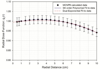
Calculated $\mathrm{M}-15$ radial dose function, ${\mathrm{g}}_{\mathrm{L}}$(r), presented at distances between 0.5 and 10 cm. These data were fit to a 5th order polynomial, as recommended in TG‐43U1, and fit to a double exponential function, as discussed by Furhang and Anderson, ⁽¹⁶⁾ for better accuracy when extrapolating outside of the measured data.

D. Anisotropy function, $\mathbf{F}(\mathbf{r},\theta ),{\varphi }_{\text{an}}(\mathbf{r})$, and ${\overline{\varphi }}_{\text{an}}$

The anisotropy function, $\mathrm{F}(\mathrm{r},\theta )$ was calculated using the TG‐43U1 equation:

$$F(r,\theta )=\frac{\dot{D}(r,\theta )}{\dot{D}(r,{\theta }_0)}\frac{G_L(r,{\theta }_0)}{G_L(r,\theta )}$$ (9)

The uncertainty in the anisotropy function, $F(r,\theta )$ was calculated using the equation derived by Medich et al.:(⁹)

$${\sigma }_F^{absolute}(r,\theta )=F(r,\theta )\sqrt{{({\sigma }_{MonteCarlo}^{relative}(r,\theta ))}^2+{({\sigma }_{MonteCarlo}^{relative}(r_{0,}{\theta }_0))}^2+2{({\sigma }_{cross\text{sec}tion}^{relative})}^2}$$ (10)

The results of these calculations are presented in Table 5 and Fig 4.

Table 5.

Calculated anisotropy function, $\mathrm{F}(\mathrm{r},\theta )$, and anisotrpy factor, ${\varphi }_{\text{an}}(\mathrm{r})$, and their absolute uncertainties for $\mathrm{M}-15$ $\text{Iridium}-192$.

$r(cm)\hspace{0.17em}\theta (deg)$	0.5	1	2.0	3.0	4.0	5.0	6.0	7.0	8.0	9.0	10.0
0	$0.660\pm 0.014$	$0.624\pm 0.014$	$0.633\pm 0.014$	$0.659\pm 0.014$	$0.684\pm 0.015$	$0.705\pm 0.015$	$0.721\pm 0.016$	$0.738\pm 0.016$	$0.751\pm 0.016$	$0.763\pm 0.016$	$0.776\pm 0.017$
1	$0.665\pm 0.014$	$0.630\pm 0.013$	$0.641\pm 0.014$	$0.664\pm 0.014$	$0.684\pm 0.015$	$0.707\pm 0.015$	$0.724\pm 0.015$	$0.743\pm 0.016$	$0.753\pm 0.016$	$0.766\pm 0.016$	$0.779\pm 0.017$
2	$0.663\pm 0.014$	$0.633\pm 0.013$	$0.648\pm 0.014$	$0.670\pm 0.014$	$0.696\pm 0.015$	$0.712\pm 0.015$	$0.728\pm 0.016$	$0.753\pm 0.016$	$0.759\pm 0.016$	$0.775\pm 0.017$	$0.779\pm 0.017$
3	$0.661\pm 0.014$	$0.642\pm 0.014$	$0.661\pm 0.014$	$0.685\pm 0.015$	$0.707\pm 0.015$	$0.727\pm 0.015$	$0.742\pm 0.016$	$0.753\pm 0.016$	$0.772\pm 0.016$	$0.783\pm 0.017$	$0.789\pm 0.017$
4	$0.668\pm 0.014$	$0.649\pm 0.014$	$0.670\pm 0.014$	$0.696\pm 0.015$	$0.715\pm 0.015$	$0.732\pm 0.016$	$0.749\pm 0.016$	$0.768\pm 0.016$	$0.779\pm 0.017$	$0.791\pm 0.017$	$0.800\pm 0.017$
5	$0.674\pm 0.014$	$0.667\pm 0.014$	$0.684\pm 0.015$	$0.706\pm 0.015$	$0.723\pm 0.015$	$0.742\pm 0.016$	$0.760\pm 0.016$	$0.773\pm 0.016$	$0.779\pm 0.017$	$0.791\pm 0.017$	$0.810\pm 0.017$
6	$0.690\pm 0.015$	$0.679\pm 0.015$	$0.695\pm 0.015$	$0.716\pm 0.015$	$0.734\pm 0.016$	$0.752\pm 0.016$	$0.763\pm 0.016$	$0.783\pm 0.017$	$0.792\pm 0.017$	$0.800\pm 0.017$	$0.810\pm 0.017$
7	$0.701\pm 0.015$	$0.696\pm 0.015$	$0.712\pm 0.015$	$0.729\pm 0.016$	$0.747\pm 0.016$	$0.762\pm 0.016$	$0.774\pm 0.017$	$0.788\pm 0.017$	$0.798\pm 0.017$	$0.808\pm 0.017$	$0.821\pm 0.017$
8	$0.714\pm 0.015$	$0.706\pm 0.015$	$0.724\pm 0.015$	$0.744\pm 0.016$	$0.759\pm 0.016$	$0.774\pm 0.016$	$0.785\pm 0.017$	$0.797\pm 0.017$	$0.805\pm 0.017$	$0.816\pm 0.017$	$0.831\pm 0.018$
9	$0.729\pm 0.015$	$0.720\pm 0.015$	$0.736\pm 0.016$	$0.753\pm 0.016$	$0.767\pm 0.016$	$0.784\pm 0.017$	$0.792\pm 0.017$	$0.807\pm 0.017$	$0.818\pm 0.017$	$0.825\pm 0.018$	$0.831\pm 0.018$
10	$0.740\pm 0.016$	$0.734\pm 0.016$	$0.749\pm 0.016$	$0.765\pm 0.016$	$0.780\pm 0.017$	$0.793\pm 0.017$	$0.804\pm 0.017$	$0.815\pm 0.017$	$0.824\pm 0.017$	$0.832\pm 0.018$	$0.840\pm 0.018$
15	$0.801\pm 0.017$	$0.796\pm 0.017$	$0.807\pm 0.017$	$0.818\pm 0.017$	$0.829\pm 0.018$	$0.838\pm 0.018$	$0.846\pm 0.018$	$0.854\pm 0.018$	$0.860\pm 0.018$	$0.867\pm 0.018$	$0.872\pm 0.019$
20	$0.848\pm 0.018$	$0.844\pm 0.018$	$0.851\pm 0.018$	$0.859\pm 0.018$	$0.867\pm 0.018$	$0.874\pm 0.019$	$0.879\pm 0.019$	$0.885\pm 0.019$	$0.889\pm 0.019$	$0.894\pm 0.019$	$0.898\pm 0.019$
25	$0.884\pm 0.019$	$0.880\pm 0.019$	$0.885\pm 0.019$	$0.891\pm 0.019$	$0.896\pm 0.019$	$0.901\pm 0.019$	$0.905\pm 0.019$	$0.909\pm 0.019$	$0.913\pm 0.019$	$0.916\pm 0.019$	$0.919\pm 0.020$
30	$0.911\pm 0.019$	$0.908\pm 0.019$	$0.911\pm 0.019$	$0.915\pm 0.019$	$0.919\pm 0.020$	$0.923\pm 0.020$	$0.926\pm 0.020$	$0.929\pm 0.020$	$0.931\pm 0.020$	$0.933\pm 0.020$	$0.935\pm 0.020$
35	$0.932\pm 0.020$	$0.929\pm 0.020$	$0.931\pm 0.020$	$0.934\pm 0.020$	$0.937\pm 0.020$	$0.940\pm 0.020$	$0.942\pm 0.020$	$0.944\pm 0.020$	$0.946\pm 0.020$	$0.947\pm 0.020$	$0.949\pm 0.020$
40	$0.948\pm 0.020$	$0.946\pm 0.020$	$0.947\pm 0.020$	$0.950\pm 0.020$	$0.951\pm 0.020$	$0.953\pm 0.020$	$0.955\pm 0.020$	$0.956\pm 0.020$	$0.958\pm 0.020$	$0.959\pm 0.020$	$0.960\pm 0.020$
45	$0.961\pm 0.020$	$0.959\pm 0.020$	$0.960\pm 0.020$	$0.962\pm 0.020$	$0.963\pm 0.020$	$0.964\pm 0.021$	$0.966\pm 0.021$	$0.967\pm 0.021$	$0.968\pm 0.021$	$0.968\pm 0.021$	$0.969\pm 0.021$
50	$0.971\pm 0.021$	$0.970\pm 0.021$	$0.970\pm 0.021$	$0.971\pm 0.021$	$0.972\pm 0.021$	$0.973\pm 0.021$	$0.974\pm 0.021$	$0.975\pm 0.021$	$0.975\pm 0.021$	$0.976\pm 0.021$	$0.976\pm 0.021$
55	$0.979\pm 0.021$	$0.978\pm 0.021$	$0.979\pm 0.021$	$0.979\pm 0.021$	$0.980\pm 0.021$	$0.981\pm 0.021$	$0.981\pm 0.021$	$0.982\pm 0.021$	$0.982\pm 0.021$	$0.983\pm 0.021$	$0.983\pm 0.021$
60	$0.985\pm 0.021$	$0.984\pm 0.021$	$0.985\pm 0.021$	$0.986\pm 0.021$	$0.986\pm 0.021$	$0.987\pm 0.021$	$0.987\pm 0.021$	$0.987\pm 0.021$	$0.988\pm 0.021$	$0.988\pm 0.021$	$0.988\pm 0.021$
65	$0.990\pm 0.021$	$0.990\pm 0.021$	$0.990\pm 0.021$	$0.990\pm 0.021$	$0.991\pm 0.021$	$0.991\pm 0.021$	$0.991\pm 0.021$	$0.992\pm 0.021$	$0.992\pm 0.021$	$0.992\pm 0.021$	$0.992\pm 0.021$
70	$0.993\pm 0.021$	$0.994\pm 0.021$	$0.994\pm 0.021$	$0.994\pm 0.021$	$0.995\pm 0.021$	$0.995\pm 0.021$	$0.995\pm 0.021$	$0.995\pm 0.021$	$0.995\pm 0.021$	$0.995\pm 0.021$	$0.995\pm 0.021$
75	$0.996\pm 0.021$	$0.996\pm 0.021$	$0.997\pm 0.021$	$0.997\pm 0.021$	$0.997\pm 0.021$	$0.997\pm 0.021$	$0.997\pm 0.021$	$0.997\pm 0.021$	$0.998\pm 0.021$	$0.997\pm 0.021$	$0.997\pm 0.021$
80	$0.998\pm 0.021$	$0.998\pm 0.021$	$0.999\pm 0.021$	$0.999\pm 0.021$	$0.999\pm 0.021$	$0.999\pm 0.021$	$0.999\pm 0.021$	$0.999\pm 0.021$	$0.999\pm 0.021$	$0.999\pm 0.021$	$0.999\pm 0.021$
85	$0.999\pm 0.021$	$1.000\pm 0.021$	$0.999\pm 0.021$	$1.000\pm 0.021$	$1.000\pm 0.021$	$1.000\pm 0.021$	$1.000\pm 0.021$	$1.000\pm 0.021$	$1.000\pm 0.021$	$1.000\pm 0.021$	$1.000\pm 0.021$
90	1.000	1.000	1.000	1.000	1.000	1.000	1.000	1.000	1.000	1.000	1.000
95	$1.000\pm 0.021$	$1.000\pm 0.021$	$0.999\pm 0.021$	$1.000\pm 0.021$	$1.000\pm 0.021$	$1.000\pm 0.021$	$1.000\pm 0.021$	$1.000\pm 0.021$	$1.000\pm 0.021$	$1.000\pm 0.021$	$1.000\pm 0.021$
100	$0.998\pm 0.021$	$0.998\pm 0.021$	$0.999\pm 0.021$	$0.999\pm 0.021$	$0.999\pm 0.021$	$0.999\pm 0.021$	$0.999\pm 0.021$	$0.999\pm 0.021$	$0.999\pm 0.021$	$0.999\pm 0.021$	$0.999\pm 0.021$
105	$0.996\pm 0.021$	$0.996\pm 0.021$	$0.997\pm 0.021$	$0.997\pm 0.021$	$0.997\pm 0.021$	$0.997\pm 0.021$	$0.997\pm 0.021$	$0.997\pm 0.021$	$0.997\pm 0.021$	$0.997\pm 0.021$	$0.997\pm 0.021$
110	$0.993\pm 0.021$	$0.994\pm 0.021$	$0.994\pm 0.021$	$0.995\pm 0.021$	$0.995\pm 0.021$	$0.995\pm 0.021$	$0.995\pm 0.021$	$0.995\pm 0.021$	$0.995\pm 0.021$	$0.995\pm 0.021$	$0.995\pm 0.021$
115	$0.990\pm 0.021$	$0.990\pm 0.021$	$0.991\pm 0.021$	$0.991\pm 0.021$	$0.991\pm 0.021$	$0.991\pm 0.021$	$0.992\pm 0.021$	$0.992\pm 0.021$	$0.992\pm 0.021$	$0.992\pm 0.021$	$0.992\pm 0.021$
120	$0.985\pm 0.021$	$0.985\pm 0.021$	$0.986\pm 0.021$	$0.986\pm 0.021$	$0.987\pm 0.021$	$0.987\pm 0.021$	$0.987\pm 0.021$	$0.987\pm 0.021$	$0.988\pm 0.021$	$0.988\pm 0.021$	$0.988\pm 0.021$
125	$0.979\pm 0.021$	$0.978\pm 0.021$	$0.979\pm 0.021$	$0.980\pm 0.021$	$0.980\pm 0.021$	$0.981\pm 0.021$	$0.981\pm 0.021$	$0.982\pm 0.021$	$0.982\pm 0.021$	$0.982\pm 0.021$	$0.983\pm 0.021$
130	$0.972\pm 0.021$	$0.970\pm 0.021$	$0.971\pm 0.021$	$0.972\pm 0.021$	$0.973\pm 0.021$	$0.974\pm 0.021$	$0.974\pm 0.021$	$0.975\pm 0.021$	$0.976\pm 0.021$	$0.976\pm 0.021$	$0.977\pm 0.021$
135	$0.962\pm 0.020$	$0.960\pm 0.020$	$0.961\pm 0.020$	$0.962\pm 0.020$	$0.963\pm 0.020$	$0.965\pm 0.021$	$0.966\pm 0.021$	$0.967\pm 0.021$	$0.967\pm 0.021$	$0.968\pm 0.021$	$0.969\pm 0.021$
140	$0.949\pm 0.020$	$0.947\pm 0.020$	$0.948\pm 0.020$	$0.950\pm 0.020$	$0.952\pm 0.020$	$0.953\pm 0.020$	$0.955\pm 0.020$	$0.956\pm 0.020$	$0.957\pm 0.020$	$0.958\pm 0.020$	$0.959\pm 0.020$
145	$0.933\pm 0.020$	$0.930\pm 0.020$	$0.932\pm 0.020$	$0.934\pm 0.020$	$0.937\pm 0.020$	$0.939\pm 0.020$	$0.941\pm 0.020$	$0.943\pm 0.020$	$0.945\pm 0.020$	$0.946\pm 0.020$	$0.948\pm 0.020$
150	$0.913\pm 0.019$	$0.908\pm 0.019$	$0.910\pm 0.019$	$0.914\pm 0.019$	$0.918\pm 0.019$	$0.921\pm 0.020$	$0.924\pm 0.020$	$0.927\pm 0.020$	$0.929\pm 0.020$	$0.932\pm 0.020$	$0.933\pm 0.020$
155	$0.885\pm 0.019$	$0.879\pm 0.019$	$0.883\pm 0.019$	$0.888\pm 0.019$	$0.893\pm 0.019$	$0.898\pm 0.019$	$0.902\pm 0.019$	$0.906\pm 0.019$	$0.910\pm 0.019$	$0.913\pm 0.019$	$0.915\pm 0.019$
160	$0.847\pm 0.018$	$0.839\pm 0.018$	$0.845\pm 0.018$	$0.853\pm 0.018$	$0.861\pm 0.018$	$0.868\pm 0.018$	$0.874\pm 0.019$	$0.880\pm 0.019$	$0.885\pm 0.019$	$0.889\pm 0.019$	$0.893\pm 0.019$
165	$0.793\pm 0.017$	$0.784\pm 0.017$	$0.794\pm 0.017$	$0.806\pm 0.017$	$0.817\pm 0.017$	$0.827\pm 0.018$	$0.836\pm 0.018$	$0.843\pm 0.018$	$0.851\pm 0.018$	$0.857\pm 0.018$	$0.863\pm 0.018$
170	$0.711\pm 0.015$	$0.701\pm 0.015$	$0.718\pm 0.015$	$0.736\pm 0.016$	$0.753\pm 0.016$	$0.768\pm 0.016$	$0.782\pm 0.017$	$0.793\pm 0.017$	$0.804\pm 0.017$	$0.814\pm 0.017$	$0.822\pm 0.017$
171	$0.691\pm 0.015$	$0.684\pm 0.014$	$0.705\pm 0.015$	$0.724\pm 0.015$	$0.740\pm 0.016$	$0.757\pm 0.016$	$0.771\pm 0.016$	$0.788\pm 0.017$	$0.792\pm 0.017$	$0.800\pm 0.017$	$0.810\pm 0.017$
172	$0.669\pm 0.014$	$0.660\pm 0.014$	$0.682\pm 0.015$	$0.705\pm 0.015$	$0.726\pm 0.015$	$0.744\pm 0.016$	$0.756\pm 0.016$	$0.773\pm 0.016$	$0.785\pm 0.017$	$0.791\pm 0.017$	$0.810\pm 0.017$
173	$0.645\pm 0.014$	$0.640\pm 0.014$	$0.663\pm 0.014$	$0.687\pm 0.015$	$0.707\pm 0.015$	$0.727\pm 0.015$	$0.746\pm 0.016$	$0.763\pm 0.016$	$0.772\pm 0.016$	$0.783\pm 0.017$	$0.800\pm 0.017$
174	$0.626\pm 0.013$	$0.618\pm 0.013$	$0.643\pm 0.014$	$0.671\pm 0.014$	$0.693\pm 0.015$	$0.712\pm 0.015$	$0.731\pm 0.016$	$0.748\pm 0.016$	$0.759\pm 0.016$	$0.775\pm 0.016$	$0.789\pm 0.017$
175	$0.615\pm 0.013$	$0.600\pm 0.013$	$0.628\pm 0.013$	$0.656\pm 0.014$	$0.679\pm 0.014$	$0.703\pm 0.015$	$0.721\pm 0.015$	$0.738\pm 0.016$	$0.753\pm 0.016$	$0.758\pm 0.016$	$0.779\pm 0.017$
176	$0.608\pm 0.013$	$0.590\pm 0.013$	$0.611\pm 0.013$	$0.636\pm 0.014$	$0.660\pm 0.014$	$0.685\pm 0.015$	$0.706\pm 0.015$	$0.724\pm 0.015$	$0.733\pm 0.016$	$0.750\pm 0.016$	$0.768\pm 0.016$
177	$0.600\pm 0.013$	$0.577\pm 0.012$	$0.607\pm 0.013$	$0.631\pm 0.013$	$0.659\pm 0.014$	$0.678\pm 0.014$	$0.699\pm 0.015$	$0.719\pm 0.015$	$0.733\pm 0.016$	$0.741\pm 0.016$	$0.758\pm 0.016$
178	$0.607\pm 0.013$	$0.571\pm 0.012$	$0.593\pm 0.013$	$0.621\pm 0.013$	$0.643\pm 0.014$	$0.671\pm 0.014$	$0.692\pm 0.015$	$0.714\pm 0.015$	$0.727\pm 0.015$	$0.733\pm 0.016$	$0.758\pm 0.016$
179	$0.610\pm 0.013$	$0.572\pm 0.012$	$0.589\pm 0.012$	$0.610\pm 0.013$	$0.637\pm 0.014$	$0.668\pm 0.014$	$0.681\pm 0.015$	$0.704\pm 0.015$	$0.714\pm 0.015$	$0.733\pm 0.016$	$0.747\pm 0.016$
180	$0.604\pm 0.013$	$0.563\pm 0.012$	$0.580\pm 0.013$	$0.604\pm 0.013$	$0.632\pm 0.014$	$0.654\pm 0.014$	$0.678\pm 0.015$	$0.698\pm 0.015$	$0.713\pm 0.015$	$0.730\pm 0.016$	$0.741\pm 0.016$
${\varphi }_{\text{an}}(\mathrm{r})$	$1.009\pm 0.015$	$0.971\pm 0.014$	$0.963\pm 0.014$	$0.964\pm 0.014$	$0.965\pm 0.014$	$0.966\pm 0.014$	$0.967\pm 0.014$	$0.968\pm 0.014$	$0.969\pm 0.014$	$0.970\pm 0.014$	$0.971\pm 0.014$

Figure 4.

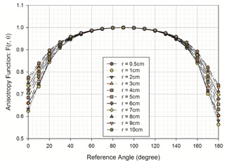
Resulting anisotropy function, $\mathrm{F}(\mathrm{r},\theta )$, of the model $\mathrm{M}-15$ source at angles between 0° and 180° and for depths between 0.5 cm to 10 cm.

The anisotropy factor, ${\varphi }_{\text{an}}(\mathrm{r})$ was also calculated using the formula:

$${\varphi }_{an}(r)=\frac{{\displaystyle {\int }_0^{\pi }\dot{D}(r,\theta )\text{sin}(\theta )d\theta }}{2\dot{D}(r,{\theta }_0)}$$ (11)

The absolute uncertainty in ${\varphi }_{\text{an}}(\mathrm{r})$ was calculated ⁽⁹⁾ as:

$$({{\sigma }_{{\phi }_{an}}^{\mathit{\text{absolute}}})}^2(r)={\left[{\phi }_{an}(r)-\frac{\Delta \theta }{2}\right]}^2[{\sigma }_{R_{\mathit{\text{tally}}}}^{\mathit{\text{relative}}}({r,{\theta }_0)]}^2+\sum _{\genfrac{}{}{0ex}{}{\theta =0}{\theta \ne {\theta }_0}}^{\pi }{\left(\frac{\dot{D}(r,\theta )}{\dot{D}(r,{\theta }_0)}\frac{\text{sin}(\theta )}{2}\Delta \theta \right)}^2[{\sigma }_{R_{\mathit{\text{tally}}}}^{\mathit{\text{relative}}}({r,\theta )]}^2$$ (12)

These results are also presented in Table 5 for the radial distance from 0.5 cm to 10 cm. From this data, the anisotropy constant was calculated to be ${\overline{\phi }}_{an}=0.969\pm 0.007$ by integrating ${\phi }_{an}(r)$ between 1 cm and 10 cm using the weighting factor ⁽⁹⁾ $w(r)=\frac{\frac{1}{r^2}}{\sum _{r=1}^{10}\frac{\mathrm{\Delta }r}{r^2}}$. The absolute uncertainty in ${\overline{\phi }}_{an}(r)$ was calculated using the equation:

$${\left({\sigma }_{{\overline{\phi }}_{an}}^{absolute}\right)}^2={\displaystyle \sum _{r=1}^{10}{[w(r)\Delta r]}^2}{\sigma }_{{\phi }_{an}}^2(r)$$ (13)

E. $\dot{\mathrm{D}}({\mathbf{r}}_0,{\theta }_0),{\mathbf{S}}_{\mathbf{k}}$, and Λ

The Monte Carlo calculated reference dose rate in water $\dot{\mathrm{D}}({\mathrm{r}}_0,{\theta }_0),\equiv \dot{\mathrm{D}}(1\text{cm},\pi /2)$ was determined to be $\dot{\mathrm{D}}({\mathrm{r}}_0,{\theta }_0)=4.038\pm 0.064\hspace{0.17em}{\text{cGy mCi}}^{-1}{\mathrm{h}}^{-1}$. The absolute uncertainty in $\dot{\mathrm{D}}({\mathrm{r}}_0,{\theta }_0)$ was calculated using Eq. (3).

The air‐kerma in free space, ${\mathrm{S}}_{\mathrm{k}}$ was reported to be $3.632\hspace{0.17em}{\text{cGy cm}}^2\hspace{0.17em}{\text{mCi}}^{-1}\hspace{0.17em}{\mathrm{h}}^{-1}$. The absolute uncertainty in ${\mathrm{S}}_{\mathrm{k}}$ was calculated to be ${\sigma }_{{\mathrm{S}}_{\mathrm{k}}}^{\text{absolute}}=0.086\hspace{0.17em}{\text{cGy cm}}^2\hspace{0.17em}{\text{mCi}}^{-1}\hspace{0.17em}{\mathrm{h}}^{-1}$ using the following equation:

$${\sigma }_{S_k}^{absolute}=S_k\sqrt{{\left({\sigma }_{MonteCarlo}^{relative}\right)}^2+{\left({\sigma }_{cross\text{sec}tion}^{relative}\right)}^2+{\left({\sigma }_{I_{\gamma }}^{relative}\right)}^2}$$ (14)

From the above data, the dose rate constant can be calculated using:

$$\Lambda =\frac{\dot{D}(r_0,{\theta }_0)}{S_K}$$ (15)

The reported dose rate constant Λ is $\Lambda =1.112\hspace{0.17em}cGy\hspace{0.17em}{h}^{-1}\hspace{0.17em}{U}^{-1}$. The absolute uncertainty has been calculated to be using the following ${\sigma }_{\Lambda }^{\text{absolute}}=0.029\hspace{0.17em}{\text{cGy h}}^{-1}\hspace{0.17em}{\mathrm{h}}^{-1}{\mathrm{U}}^{-1}$ using the following equation:

$${\sigma }_{\Lambda }^{absolute}=\Lambda \sqrt{{({\sigma }_{R_{tally}}^{relative}(r_0,{\theta }_0))}^2+{({\sigma }_{R_{air\hspace{0.17em}\text{ker}ma}^{\delta =10}}^{relative})}^2}$$ (16)

IV. CONCLUSIONS

A dosimetric study of the $\mathrm{M}-15$ $\text{Iridium}-192$ HDR brachytherapy source was performed using the MCNP6 radiation transport code. The dose rate constant, radial dose function, and anisotropy function were calculated in accordance with the updated AAPM and ESTRO dosimetric parameters for brachytherapy sources of average energy greater than 50 keV. These data, therefore, may be applied toward clinical use and toward the development of a treatment program.

REFERENCES

- 1. Hammer J, Seewald DH, Track C, Zoidl JP, Labeck W. Breast cancer: primary treatment with external‐beam radiation therapy and high‐dose‐rate iridium implantation. Radiology. 1994;193(2):573–77. [DOI] [PubMed] [Google Scholar]
- 2. Kapp KS, Stuecklschweiger GF, Kapp DS, Poschauko J, Pickel H, Hackl A. Carcinoma of the cervix: analysis of complications after primary external beam radiation and Ir‐192 HDR brachytherapy. Radiother Oncol. 1997;42(2):143–53. [DOI] [PubMed] [Google Scholar]
- 3. Kapp KS, Stuecklschweiger GF, Kapp DS, et al. Prognostic factors in patients with carcinoma of the uterine cervix treated with external beam irradiation and IR‐192 high‐dose‐rate brachytherapy. Int J Radiat Oncol Biol Phys. 1998;42(3):531–40. [DOI] [PubMed] [Google Scholar]
- 4. Nag S. High dose rate brachytherapy: its clinical applications and treatment guidelines. Technol Cancer Res Treat. 2004;3(3):269–87. [DOI] [PubMed] [Google Scholar]
- 5. Schmidt‐Ullrich R, Zwicker RD, Wu A, Kelly K. Interstitial IR‐192 implants of the oral cavity: the planning and construction of volume implants. Int J Radiat Oncol Biol Phys. 1991;20(5):1079–85. [DOI] [PubMed] [Google Scholar]
- 6. Perez‐Calatayud J, Ballester F, Das RK, et al. Dose calculation for photon‐emitting brachytherapy sources with average energy higher than 50 keV: report of the AAPM and ESTRO. Med Phys. 2012;39(5):2904–29. [DOI] [PubMed] [Google Scholar]
- 7. Rivard MJ, Coursey BM, DeWerd LA, et al. Update of AAPM Task Group No. 43 Report: a revised AAPM protocol for brachytherapy dose calculations. Med Phys. 2004;31(3):633–74. [DOI] [PubMed] [Google Scholar]
- 8. Pelowitz D, editor. MCNP6 user manual, Version 1.0. Report No. LA‐CP‐13‐00634. Los Alamos, NM: Los Alamos National Laboratory; 2013. [Google Scholar]
- 9. Medich DC, Tries MA, Munro JJ. Monte Carlo characterization of an ytterbium‐169 high dose rate brachytherapy source with analysis of statistical uncertainty. Med Phys. 2006;33(1):163–72. [DOI] [PubMed] [Google Scholar]
- 10. Medich DC and Munro JJ III. Monte Carlo characterization of the M‐19 high dose rate Iridium‐192 brachytherapy source. Med Phys. 2007;34(6):1999–2006. [DOI] [PubMed] [Google Scholar]
- 11. Melhus CS and Rivard MJ. Approaches to calculating AAPM TG‐43 brachytherapy dosimetry parameters for 137Cs, 125I, 192Ir, 103Pd, and 169Yb sources. Med Phys. 2006;33(6):1729–37. [DOI] [PubMed] [Google Scholar]
- 12. Firestone RB and Ekström LP. WWW table of radioactive isotopes. 2004. Available from: http://ie.lbl.gov/toi/perchart.htm
- 13. Perez‐Calatayud J, Granero D, Ballester F. Phantom size in brachytherapy source dosimetric studies. Med Phys. 2004;31(7):2075–81. [DOI] [PubMed] [Google Scholar]
- 14. Hubbell JH and Seltzer SM. Tables of x‐ray mass attenuation coefficients and mass energy‐absorption coerricients (version 1.03). 1997. Available from: http://physics.nist.gov/PhysRefData/XrayMassCoef/cover.html
- 15. Berger MJ, Coursey JS, Zucker MA, Chang J. Stopping‐power and range tables for electrons, protons, and helium ions. 2000. Available from: http://physics.nist.gov/PhysRefData/Star/Text/contents.html
- 16. Furhang EE and Anderson LL. Functional fitting of interstitial brachytherapy dosimetry data recommended by the AAPM Radiation Therapy Committee Task Group 43. American Association of Physicists in Medicine. Med Phys. 1999;26(2):153–60. [DOI] [PubMed] [Google Scholar]