Continuum Reconfigurable Parallel Robots for Surgery: Shape Sensing and State Estimation with Uncertainty

Abstract

This paper examines shape sensing for a new class of surgical robot that consists of parallel flexible structures that can be reconfigured inside the human body. Known as CRISP robots, these devices provide access to the human body through needle-sized entry points, yet can be configured into truss-like structures capable of dexterous movement and large force application. They can also be reconfigured as needed during a surgical procedure. Since CRISP robots are elastic, they will deform when subjected to external forces or other perturbations. In this paper, we explore how to combine sensor information with mechanics-based models for CRISP robots to estimate their shapes under applied loads. The end result is a shape sensing framework for CRISP robots that will enable future research on control under applied loads, autonomous motion, force sensing, and other robot behaviors.

I. Introduction

CONTINUUM Reconfigurable Incisionless Surgical Parallel (CRISP) robots combine the stiffness advantages of parallel robots with the adaptability of reconfigurable robots [1]. Their thin elements can pass through needle-size body entry points, making them highly minimally invasive. Because the elements bend continuously like continuum robots, CRISP robots must be described by mechanics-based models that can accommodate large deflection. We proposed the CRISP concept for the first time in [1], and discussed a variety of potential applications for it in thoracic and abdominal surgery (e.g., a compelling application is percutaneous closed-chest lung biopsy and intervention). This paper addresses the problem of integrating sensing with these large-deflection models in order to determine the robot’s configuration when an external load or other disturbance is applied.

CRISP devices lie at the intersection of continuum, parallel, and reconfigurable robotics, and combine a number of their advantages in a way that is beneficial in surgical scenarios. Continuum robots are largely motivated by the problem of manipulation in confined, hard-to-reach workspaces. Unlike rigid-link robots, continuum robots can continuously deform along their body [2]. Continuum devices have been applied to the applications of exploration [3] and medicine [4]. Parallel robots differ from classical serial-link manipulators in that they are composed of closed kinematic chains [5]. Because of this structure, parallel robots are stiff mechanisms that can carry high payloads compared to serial-link devices. Reconfigurable robots are motivated by the frustration of trade-offs during the design of robot systems [6]. Reconfigurable devices can change their morphology to satisfy changing task requirements without redesigning the device. The CRISP concept melds the reach of continuum robots with the stiffness of parallel robots and the reconfigurability of reconfigurable robots.

A particular motivation that inspired the CRISP concept was the recognition that the process of designing continuum robots is fraught with trade-offs. Designers can choose between actuation methods such as tendons [7], pneumatics [8], concentric-tubes [9], [10], and antagonistic backbones [11]. These decisions govern the robot’s workspace, dexterity, and stiffness. Formal design methods for continuum robots often incorporate planning [12] and numerical optimization [13], resulting in highly task-optimized devices. It is challenging to design continuum robots for tasks whose requirements change. In minimally-invasive surgical applications, robots must be able to reach large workspaces that dynamically change as tissue is deformed or resected, yet also apply large forces that cannot be fully characterized a priori. Using traditional designs, one cannot simultaneously optimize all constraints, forcing the optimization of one at the expense of others.

The desire to avoid having to make so many tradeoffs recently motivated the development of the Continuum Reconfigurable Incisionless Surgical Parallel (CRISP) robot concept [1]. CRISP systems consist of multiple needle-diameter (< 3 mm) devices that are inserted through the skin and assembled into parallel structures in the body using snares (Fig. 1(a)). The base of each needle-diameter element is attached to and controlled by a robot manipulator. The CRISP concept is well-suited for a robotic approach because the required motions of the robot manipulators to achieve the desired motion of the surgical instrument inside the body are physically well-defined but not necessarily intuitive. For an example of the trajectory motion of a CRISP system, see [1].

Fig. 1.

The Continuum Reconfigurable Incisionless Surgical Parallel (CRISP) concept lies at the intersection of parallel [5], continuum [2], and reconfigurable [6] robotics. (a) CRISP devices are parallel structures consisting of a needle-diameter flexible tool that is grasped by multiple needle-diameter snare devices. The snare devices are positioned using manipulators. (b) This paper addresses the problem of shape sensing and state estimation for CRISP systems using uncertain kinematic models and noisy sensors.

The CRISP concept takes the benefits of continuum robots (e.g., their small size makes them favorable for minimally-invasive therapy [4]) and combines them with the benefits of parallel robots (e.g., their rigid structure [5]). CRISP systems also take the benefits of reconfigurable robots [6] with the unique ability to reconfigure their parallel structures inside the patient’s body in a way that selectively adjusts their properties (e.g., workspace, stiffness, etc.) to meet changing task requirements. The CRISP concept’s parallel structure, its ability to reconfigure, and its ability to deploy inside the body without incisions, make it a unique concept within the surgical robotics community. Potential applications include the biopsy and ablation of lung tumors, fetal surgery, and neonatal surgery (for additional discussion of motivating clinical applications, see [1]).

This paper examines the problem of state and shape estimation for CRISP robots ((Fig. 1(b)). Our work is motivated by the fact that the needle-diameter continuum elements that make up the structure are continuously flexible and a physician will want to know the structure’s shape for safe operation near sensitive tissue in the presence of uncertainty. Uncertainty can result from unmodeled friction or uncertainty in the tool and snare needles’ base poses relative to the workspace (i.e., system inputs). Adding sensors to the system can reduce uncertainty, even though sensor observations can be subject to uncertainty themselves. Sensors that can be used with continuum robots are also appropriate for the CRISP concept. Clinically relevant sensors include electromagnetic tracking sensors [14], optical tracking systems [15], and fiber Bragg-grating (FBG) sensors [16]. In the remainder of this paper we extend concepts originally developed for continuum robots in [17] to CRISP systems that enable powerful classical estimation techniques to be used to reason about a CRISP system’s state in the presence of uncertainty.

II. Sensing for CRISP Systems

We use a notation where matrices are written in upper-case standard-font (e.g., M), vectors are written in bold, lower-case font (e.g., v), and scalars are written in lower-case standard font (e.g., s). We use $\mathcal{N}(\mathit{m},\sum )$ to denote a Guassian random distribution with mean vector m and covariance matrix Σ. Many variables in this paper are functions of a scalar arc-length parameter s. We use subscript notation to denote s as a function argument. For example, if x is a function of s, then it is written as x_s rather than x(s). Note that we assume the CRISP model is quasi-static, which is assumed for other flexible robot models (e.g., concentric tube robots [9], [10] and flexible multi-backbone robots [18]).

A. Modeling CRISP Kinematics

The kinematics of CRISP systems was first presented in [1]; however, we report the kinematics herein for completeness. The flexible tool and the snare needles of a CRISP system are modeled as unshearable and inextensible Cosserat rods, whose states consist of a backbone position p ∈ ℝ³, an orientation quaternion q ∈ ℍ, an internal moment m ∈ ℝ³, and an internal force n ∈ ℝ³. The total state of a CRISP system consists of the Cosserat rod states of the tool x_t and n snare needles x₁ … x_n packed into the vector

$$\mathit{x}={\left[\begin{array}{llll}{\mathit{x}}_{\mathit{t}}\hfill & {\mathit{x}}_1\hfill & \dots \hfill & {\mathit{x}}_{\mathit{n}}\hfill \end{array}\right]}^{\top }$$ (1)

which varies with arc-length parameter s by the derivative

$$\mathit{x}\prime ={\left[\begin{array}{llll}{\mathit{x}}_{\mathit{t}}^{\prime }\hfill & {\mathit{x}}_1^{\prime }\hfill & \dots \hfill & {\mathit{x}}_n^{\prime }\hfill \end{array}\right]}^{\top }=\mathit{f}(\mathit{x},s),$$ (2)

where the function f is described in Appendix A.

The differential equation (2) is defined on the arc-length interval [s_min s_max] with endpoints defined as

$$s_{min}=min\{0,s_1-{\ell }_1,\dots ,s_n-{\ell }_n\}\text{and}{s}_{max}={\ell }_t,$$ (3)

where s₁ … s_n are the snare grasp point locations measured from the tool’s base, and ℓ_t and ℓ₁ … ℓ_n are the lengths of the tool and snare needles, respectively.

A set of geometric and mechanic constraints governs the kinematics of CRISP systems. First, we encode the system “inputs” as a constraint on the initial pose where p_td and q_td represent the desired initial position and quaternion of the flexible tool at arc-length s_min, and p_id and q_id represent the desired initial position and quaternion of the i^th snare needle at arc-length s_min. Second, we assume that the tip of the tool is load- and moment-free. Third, at the arc-length location s_i where the i^th snare needle grasps the tool, we assume that their backbone positions are coincident (i.e., the distal tip of the snare needle contacts the tool backbone, which is enforced by the snare wire) and that the snare needle and tool orientations are orthogonal. We also assume that the grasp cannot support moments in the ${\mathit{p}}_{\mathit{t}}^{\prime }$ and ${\mathit{p}}_{\mathit{i}}^{\prime }$ directions.

The constraints for the flexible tool are represented as

$${\mathit{c}}_{\mathit{t}\mathit{u}}(s_{min})=\left[\begin{array}{ll}{\mathit{p}}_{\mathit{t}}-{\mathit{p}}_{\mathit{t}\mathit{d}}\hfill & \text{initial position}\hfill \\ \log ({\mathit{q}}_{\mathit{t}}{\mathit{q}}_{\mathit{t}\mathit{d}}^{-1})\hfill & \text{initial quaternion}\hfill \end{array}\right]=\mathbf{0}$$ (4)

$${\mathit{c}}_{\mathit{t}\mathit{l}}({\ell }_t)=\left[\begin{array}{ll}{\mathit{m}}_{\mathit{t}}\hfill & \text{tip moment-free}\hfill \\ {\mathit{n}}_{\mathit{t}}\hfill & \text{tip force-free}\hfill \end{array}\right]=\mathbf{0}.$$ (5)

The initial pose constraints c_ui for each snare needle are defined equivalently as (4), and the grasp constraints are

$${\mathit{c}}_{\mathit{i}}(s_i)=\left[\begin{array}{ll}{\mathit{p}}_{\mathit{t}}-{\mathit{p}}_{\mathit{i}}\hfill & \text{tip coincidence}\hfill \\ {\mathit{p}}_{\mathit{t}}^{\prime }\cdot {\mathit{p}}_{\mathit{i}}^{\prime }\hfill & \text{shaft orthogonality}\hfill \\ {\mathit{p}}_{\mathit{i}}^{\prime }\cdot {\mathit{m}}_{\mathit{i}}\hfill & \text{needle shaft moment}\hfill \\ {\mathit{p}}_{\mathit{t}}^{\prime }\cdot {\mathit{m}}_{\mathit{i}}\hfill & \text{tool shaft moment}\hfill \end{array}\right]=\mathbf{0}.$$ (6)

All tool and snare constraints are packed into the vector c, which is a function of the full state at multiple arc-lengths:

$$\mathit{c}={[\begin{array}{lllllll}{\mathit{c}}_{\mathit{t}\mathit{u}}\hfill & {\mathit{c}}_{\mathit{t}}\hfill & {\mathit{c}}_{\mathbf{1}\mathit{u}}\hfill & {\mathit{c}}_{\mathbf{1}}\hfill & \dots \hfill & {\mathit{c}}_{\mathit{n}\mathit{u}}\hfill & {\mathit{c}}_{\mathit{n}}\hfill \end{array}]}^{\top }=\mathbf{0}.$$ (7)

Additional constraints can be created, such as to enforce remote-center motion of an element around a virtual point in space, or to compute inverse-kinematics solutions [1].

The combined differential equation (2) and constraint vector (7) form a multi-point boundary differential equation that can be numerically solved using standard methods. In this paper, we use a shooting method that numerical varies the initial states ${\mathit{x}}_{s_{min}}$ to satisfy the constraint equation (7).

B. Statistical State Estimation for CRISP Structures

The model (2) and constraints (7) are approximations that are subject to uncertainty. Uncertainty in the system is modeled with zero-mean additive process noise q_s and constraint noise w as

$$\begin{array}{lll}\mathit{x}\prime =\mathit{f}(\mathit{x},\mathit{s})+{\mathit{q}}_s\hfill & \text{and}\hfill & \mathit{c}=\mathit{w}\hfill \end{array},$$ (8)

where ${\mathit{q}}_s~\mathcal{N}(\mathbf{0},Q_s)$ and $\mathit{w}\sim \mathcal{N}(\mathbf{0},W)$. The covariance W is a block-diagonal matrix packed with covariances of the tool and snare constraints.

Uncertainty can be reduced by using sensors, even though they are also subject to uncertainty in the form of sensor noise. The goal of statistical state estimation is to infer the most likely state of a CRISP system at all arc-lengths s given uncertain sensors and models. Formulating a CRISP system’s kinematics in the form of (8) enables decades’ worth of estimation techniques to be immediately applicable to the state estimation problem for CRISP devices.

We model sensors as discrete observations along the body of a CRISP structure at arc-lengths o₁ … o_m. Noisy sensor observations ${\mathit{y}}_{o_i}$ at discrete arc-lengths o_i are given by the random process

$${\mathit{y}}_{o_i}={\mathit{h}}_{o_i}({\mathit{x}}_{o_i})+{\mathit{z}}_{o_i},$$ (9)

where the function ${\mathit{h}}_{o_i}$ models the sensor and ${\mathit{z}}_{o_i}~\mathcal{N}(\mathbf{0},Z_{o_i})$ is zero-mean random noise with covariance $Z_{o_i}$. Sensor covariances can typically be found experimentally.

The statistical estimate at arc-length s that incorporates all available model and sensor information is referred to as the “smoothed” estimate, denoted by $\mathcal{N}({\overline{\mathit{x}}}_s,{\overline{P}}_s)$ with expected value ${\overline{\mathit{x}}}_s$ and covariance ${\overline{P}}_s$. The smoothed estimate is computed by forward integrating (in arc-length s) the extended form of the Kalman-Bucy differential equations and then backward integrating the extended form of the Rauch-Tung-Striebel (RTS) smoothing differential equations.

The Kalman-Bucy equations produce the posterior estimate of a CRISP system’s state, denoted by $\mathcal{N}({\stackrel{\sim }{\mathit{x}}}_s,{\stackrel{\sim }{P}}_s)$, which is the statistical state estimate given the boundary constraints and sensor observations on the arc-length interval [s_min s_max] (see Fig. 2(a)). The Kalman-Bucy differential equations that produce the posterior state estimate are

$${\stackrel{\sim }{\mathit{x}}}_s^{\prime }=\mathit{f}({\stackrel{\sim }{\mathit{x}}}_s,s)$$ (10)

$${\stackrel{\sim }{P}}_s^{\prime }=F_s{\stackrel{\sim }{P}}_s+{\stackrel{\sim }{P}}_s{F}_s^{\top }+Q_s$$ (11)

with initial conditions ${\stackrel{\sim }{\mathit{x}}}_{s_{min}}$ and ${\stackrel{\sim }{P}}_{s_{min}}$, and where F_s = ∂f(x_s, s)/∂x_s. The initial conditions represent the initial state belief. In this case, ${\stackrel{\sim }{\mathit{x}}}_{s_{min}}$ contains the initial registration of the base pose of each element as well as estimated values for other appended parameters (see Sec. II-D).

Fig. 2.

An illustration of the information incorporated in (a) the posterior state estimate generated by the Kalman-Bucy filter at arc-length s₃, and (b) the smoothed estimate generated by the Rauch-Tung-Striebel smoother at arc-length s₃. Sensor observations are denoted by y_i. Constraints c_i are handled by the Kalman-Bucy filter as sensor observations.

A Kalman update is performed at each constraint arc-length s₁ … s_n and at each sensor observation o₁ … o_m during the forward integration. The extended Kalman update equations are given in Appendix B.

The second step in the estimation process produces the smoothed estimate $\mathcal{N}({\overline{\mathit{x}}}_s,{\overline{P}}_s)$ by integrating the RTS differential equations from the tip to the base arc-lengths. The RTS differential equations are given by

$${\stackrel{\sim }{\mathit{x}}}_s^{\prime }=\mathit{f}({\overline{\mathit{x}}}_s,s)+Q_s{\stackrel{\sim }{P}}_s^{-1}({\overline{\mathit{x}}}_s-{\stackrel{\sim }{\mathit{x}}}_s)$$ (12)

$${\overline{P}}_s^{\prime }=(F_s+Q_s{\stackrel{\sim }{P}}_s^{-1}){\overline{P}}_s+{\overline{P}}_s{(F_s+Q_s{\stackrel{\sim }{P}}_s^{-1})}^{\top }-Q_s$$ (13)

with initial conditions ${\overline{\mathit{x}}}_{\ell }={\stackrel{\sim }{\mathit{x}}}_{\ell }$ and ${\overline{P}}_{\ell }={\stackrel{\sim }{P}}_{\ell }$. The smoothed estimate incorporates all sensor and constraint information on the interval [s_min s_max] (see Fig. 2(b)).

Fig. 3(a) shows an illustration of the smoothed position covariance (a submatrix of ${\overline{P}}_s$) of a simulated two-snare CRISP structure with a position sensor placed at three locations on a 0.5 m-long flexible tool. The sensor’s placement has a substantial effect on the system’s position covariance. The sensor’s placement along the flexible tool’s body changes how informative the sensor is about the entire structure’s shape. This can be observed when contrasting the position covariance of the distal snare when the sensor is placed at the flexible tool’s base (o₁ = 0.0 m) with the distal snare’s position covariance with the sensor placed at the tool’s tip (o₁ = 0.5 m). The information that a sensor provides depends on the sensor’s noise covariance $Z_{o_i}$ (smaller being more informative) and the mechanical structure of the CRISP system (determined by the state matrix F_s).

Fig. 3.

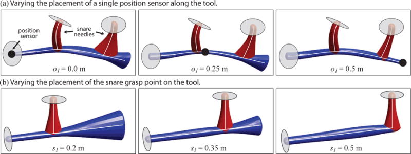
(a) A simulated two-snare CRISP structure is shown with an overlaid depiction of the smoothed position covariance as a single position sensor is moved down the length of the flexible tool. The position covariance represents the position uncertainty of the tool and snares. The placement of the sensor dramatically changes the smoothed estimate’s position uncertainty. (b) A simple CRISP structure with one snare is shown with an overlaid depiction of the smoothed position covariance as the snare and its grasp point are translated along the tool’s backbone. The snare configuration has a clear effect on the smoothed estimate’s position uncertainty, which may influence how a CRISP system is reconfigured. Note that this figure was generated with uncertainty in the snare grasp-point location on the tool’s body.

Along with sensor observations, a CRISP system’s configuration also has an important effect on its position covariance. Fig. 3(b) shows an illustration of the smoothed position covariance of a CRISP structure with one snare needle grasping the flexible tool at three different grasp points. Here, there are no sensor observations, making the smoothed covariance a function of the initial uncertainty in the system’s inputs (the tool and snare base poses). As illustrated, grasping the flexible tool at its tip (s₁ = 0.5 m) reduces the system’s overall position uncertainty despite the same initial uncertainty in the tool and snare base poses. This is a result of the CRISP system’s parallel structure and is an advantage, shared with their rigid-link parallel counterparts [5], over serial continuum and rigid-link manipulators.

Fig. 3(b) also illustrates that some CRISP configurations are more information-rich than others (this was also observed for concentric-tube continuum robots [17]). When selecting how a CRISP system should be reconfigured to meet changing application requirements, the system covariance will be an important consideration.

C. Observability Requirements

Designers of sensing systems for continuum robots must decide what sensors to use and where to place them. There are many considerations that must be made when selecting what sensors to use (e.g., size, cost, etc.). Although we do not address the advantages and disadvantages of the many sensing methods available to designers, the statistical state estimation methods of Sec. II-B require that the sensors be chosen and placed so that the CRISP system’s states are ”observable.” This condition is satisfied when any perturbation that preserves the system’s constraints can be detected in the sensor observations. This condition can be guaranteed by analyzing the rank of the system’s observability matrix

$$O({\mathit{x}}_{s_{min}})={\left[\begin{array}{lll}{Y}_{o_1}^{\top }\hfill & \dots \hfill & Y_{o_m}^{\top }\hfill \end{array}\right]}^{\top }$$ (14)

in which $Y_{o_i}=\partial {\mathit{h}}_{o_i}({\mathit{x}}_{o_i})/\partial {\mathit{x}}_{s_{min}}$. If the observability matrix $O(x_{s_{min}})$ has full rank, then the states can be locally estimated. Designers should select the number of sensors, types (i.e., position sensors, force sensors, etc.), and placements that make the observability matrix full rank.

D. Inferring Parameters from Observations

The power of the framework (10)—(13) as a tool for general estimation can be demonstrated by extending it to estimate general parameters. A parameter vector d can be inferred from noisy sensor observations and an uncertain model by augmenting the state vector x with vector d as

$$\mathit{x}={[\begin{array}{lllll}{\mathit{x}}_{\mathit{t}}\hfill & {\mathit{x}}_{\mathbf{1}}\hfill & \dots \hfill & {\mathit{x}}_{\mathit{n}}\hfill & \mathit{d}\hfill \end{array}]}^{\mathit{T}},$$ (15)

where the arc-length derivative of the parameter is d′ = 0 and augments the state derivative equation (2) in the same manner. The Kalman filter and smoother implicitly estimate the parameter d by the parameter’s effect on the linearized state matrix F_s.

Parameter estimation is a useful tool to remove the effects of non-zero-mean systematic uncertainty on the filter and smoother equations. For example, we found that the orthogonality assumption in the snare grasp constraint (6) can be relaxed by re-expressing them as

$${\mathit{P}}_{\mathit{t}}^{\prime }\cdot {\mathit{P}}_{\mathit{i}}^{\prime }-d_i=\mathbf{0}$$ (16)

and then estimating the parameter vector d = [d₁ … d_n]^T. This approach is applied in Sec. III

Parameter estimation can also be used to estimate applied loads. Discrete applied forces F_j and moments T_j at known arc-length s_j are incorporated into the kinematic model of Sec. II-A through (20) and (21) in the appendix. A force F_j at arc-length s_j can be estimated by augmenting the CRISP system state with the force F_j and updating the linearized state matrix $F_{s_j}$ at arc-length s_j accordingly.

Other parameters that can be estimated include system calibration properties (e.g., grasp-point location, rod stiffness, etc.). Many parameters can be estimated as long as the requirements for observability are satisfied.

III. Experimental Results

The estimation framework presented in Section II-B was applied to a CRISP device consisting of a flexible tool and two snare needles. The tool and snare needles were constructed out of Nitinol tubing (ID = 0.97 mm, OD = 1.27 mm, E = 50 GPa, η = 0.33). The lengths of the tool, first snare, and second snare were 500 mm, 154 mm, and 153 mm, respectively. The snare loops were made of 0.508 mm wide, 0.2794 mm thick Nitinol strip and were tensioned manually. The CRISP structure was placed into two different static configurations using articulated holders (Fig. 4(a)). The arc-length grasp point locations for the first and second snare needles were 200 mm and 400 mm, respectively. The base poses of the tool and snare needles were localized by rigid registration using a Northern Digital, Inc. Aurora electromagnetic tracking system and a set of fiducial points arranged on clear acrylic discs. The acrylic fiducial discs were placed at the base of the flexible tool and both snare needles. Six points on each disc were localized using a hand-held electromagnetic-sensor probe.

Fig. 4.

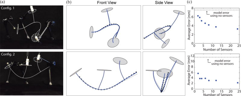
(a) The experimental CRISP structure was placed into two configurations. The snare needles and flexible tool are traced for clarity. (b) Two views of the kinematic model (grey) and smoothed state estimate (blue) plotted on top of 24 data points obtained with the electromagnetic tracker. (c) The average backbone position error (17) is shown as a function of the number of uniformly-spaced sensor observations incorporated into the smoothed estimate. The average error was computed from 100 samples and the standard deviation is smaller than the plot points.

The covariance of the tracker was measured to be isotropic with a standard deviation of 1 mm. The covariance of the base position and orientation (represented with a quaternion) was then found using the known geometry of the acrylic fiducial discs and the measured tracker covariance using the results of [19]. The estimation process was performed with no process noise (i.e., Q = 0) and the grasp covariance pseudo-measurement was estimated a priori. In all experiments, the grasp constraint was relaxed to allow the snare needle axes and flexible tool axis to violate the perpendicularity constraint as described in Sec. II-D. The numerical values of the base position and orientation covariances and the grasp covariances are omitted here for brevity.

In both configurations, the shape of the flexible tool was measured using a 0.3 mm-diameter electromagnetic 5-DOF sensor at 24 uniformly-spaced positions separated by 20 mm. Fig. 4(b) shows the raw tracker data plotted on top of the kinematic model presented in Sec. II-A and the estimated position generated by the Kalman smoother presented in Sec. II-B using all 24 data points. The accuracy of the model and smoothed estimate was measured by computing the average tool backbone error at all 24 sensor locations as

$$e(s_k)=\Vert {\mathit{p}}_{\mathit{t}}(s_k)-{\mathit{p}}_{\mathit{k}}^{\ast }\Vert$$ (17)

where s_k = [0.04,…, 0.5] are the 20 mm-spaced arc-lengths where sensor data was collected, p_t is the tool backbone position (in the model case) or the smoothed tool backbone position estimate ${\overline{\mathit{p}}}_{\mathit{t}}$ (in the smoothed case), and ${\mathit{p}}_{\mathit{k}}^{\ast }$ is the measured tool backbone position. Fig. 4(c) shows the average error of the smoothed estimate and the model after 100 trials, plotted as a function of the number of sensor observations on the flexible tool’s backbone that were incorporated into the smoothed estimate. This demonstrates how additional sensor observations improve the overall position estimate (given by the average error). However, it also shows that adding more sensors has diminishing returns in terms of error reduction; the designer should choose the number of sensors to balance accuracy with the complexity and cost of more sensors.

There is great interest in the continuum robotics community to use continuum devices as manipulators that can estimate the forces they are applying to their environment [11], [20]–[23]. Elastic continuum devices are unique compared to their rigid serial-link counterparts in that they are intrinsically compliant devices, where their physical displacement can be used as an indicator of the applied forces [11], [20]. In the case of CRISP systems, performing manipulation with the flexible tool will result in applied loads to the flexible tool’s tip. If there is a priori knowledge that a force is being applied, but the force’s magnitude and direction is unknown, then the applied force and shape can be simultaneously estimated (see Sec. II-D).

Fig. 5 shows the results of simultaneous force and shape estimation for the same configurations as Fig. 4, but with an applied load created by a 20 g mass hung 5 mm from the flexible tool’s tip. We anticipate that position accuracy will be critical for surgical tasks, even under applied loads during manipulation. Fig. 5(c) shows the average backbone position error (17) (over 100 trials) of the smoothed estimate and the model (without any sensor observations).

Fig. 5.

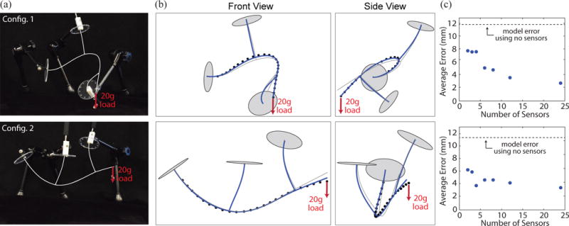
(a) The experimental CRISP structure was placed into two configurations with a 20 g load applied 5 mm from the tool’s tip. The snare needles and flexible tool are traced for clarity. (b) Two views of the kinematic model (grey) and smoothed state estimate (blue) plotted on top of 24 data points obtained with the electromagnetic tracker. (c) The average backbone position error (17) is shown as a function of the number of uniformly-spaced sensor observations incorporated into the smoothed estimate. The average error was computed from 100 samples and the standard deviation is smaller than the plot points.

The estimated applied load with no load present and with a 20 g load present is shown in Fig. 6 for the configurations of Fig. 4(a) and Fig. 5(a), respectively, as a function of the number of sensor observations incorporated in the smoothed estimate. In the case of no actual load applied, the estimator reports almost no applied load (at most less than 6.5 × 10⁻⁷ N for both configurations) as shown in Fig. 6(a). When the 20 g load is applied 5 mm from the tip of the flexible tool, the estimate under-reports the true load (Fig. 6(b)). In an analysis of observability (see Sec. II-C) we found that applied loads at the tip of the flexible tool are very difficult to distinguish from the parameters used to relax the orthogonality constraint at the grasp locations (see Sec. II-D). This indicates that uncertainty in the grasp constraints precludes the accurate estimation of tip load. Future CRISP systems that make use of force sensing must reduce uncertainty in the grasp constraints either through improved modeling or mechanical design. Note that despite under-reporting the tip-load magnitude, the estimate does correctly identify that no load is present when there is, in fact, no load applied.

Fig. 6.

(a) The estimated applied load with no actual load present for the configurations shown in Fig. 4(a), as a function of the number of sensor observations incorporated in the smoothed estimate. The estimator correctly reports there is virtually no load present when no load is actually applied. (b) The estimated applied load when a 20 g load is applied for the configurations of Fig. 5(a), as a function of the number of sensor observations incorporated in the smoothed estimate. In an observability study, we found that large uncertainty in the snare grasps can preclude the accurate estimation of applied load; uncertainty must be reduced through improved modeling or design.

We anticipate that the accuracy of the flexible tool’s tip position and heading estimates will be critical for manipulation tasks, particularly for surgical tasks where the surgeon may not be able to directly observe the tool tip. Fig. 7 shows the average position error (over 100 samples) of the smoothed estimate measured at the tool tip for varying number of sensor observations with the CRISP structure configured in the two configurations shown in Fig. 5(a). In addition, Fig. 7 reports the average angle (over 100 samples) between the measured heading obtained by the magnetic tracker system at the tool’s tip and the heading reported by the smoothed estimate and kinematic model (without any sensor observations). Note that tip position and heading was inferred by the state estimator from observations knowing the location of the applied force (5 mm from the tip) but without knowing the true magnitude or heading of the applied load. This is representative of the knowledge that a CRISP system would have if the tip is being used for manipulation tasks.

Fig. 7.

(a) The average tip position and tip heading error of the kinematic model with no sensors and the smoothed estimate measured at the tip of configuration 1 with a 20 g applied load, plotted as a function of the number of sensor observations incorporated in the smoothed estimate. (b) The average position and heading error of configuration 2 with the same load. In both examples, the state estimator does not know the direction or magnitude of the load. This demonstrates the estimator’s ability to estimate the CRISP system’s shape even in the presence of an unknown load. The average error is computed with 100 samples and the standard deviation is too small to display.

IV. Discussion and Conclusion

The smoothed covariance matrix ${\overline{P}}_s$ indicates the expected uncertainty of the system’s state estimates, given known uncertainty in the model and sensor observations. As illustrated by Fig. 3(a), varying the placement of sensor observations changes the smoothed covariance. After the requirements for observability are ensured, the smoothed covariance matrix ${\overline{P}}_s$ can be used to reduce the uncertainty of a CRISP system’s state estimates. A task-specific covariance-based metric is introduced for this purpose in [17]. This ultimately turns the problem of selecting where to place sensor observations into an optimization problem. Since the sensor observation covariances are typically known in advance, actual sensor observations are not required to obtain the smoothed covariance matrix during the computation of the metric. The smoothed covariance can be computed before sensor data is collected, enabling sensor optimization during the system design process. We expect that this approach can also be applied to sensing systems for CRISP structures, and will result in sensor placements that exploit the CRISP structure to gain as much state information as possible.

A unique aspect of the CRISP concept is that the parallel structures can be reconfigured in the body into entirely different topologies [1]. In this paper, the state estimation techniques assume that the topology—the arrangement in which the snares grasp the tool or one another—is known a priori. If this is not the case, then the kinematic model cannot be solved and the statistical state estimation cannot be performed. Future work will focus on discovering the topology of a CRISP system from sensor observations without a priori knowledge. Modular self-reconfigurable robots face a similar problem, which becomes more challenging as the number of modules is increased [6]. We anticipate that for many medical applications, a CRISP system will likely consist of no more than two snares with a total of four possible topologies.

In both experimental loaded configurations, the smoothed estimate showed a significant improvement in tip position error. For a system with four sensors, configuration 1 had a 74% improvement in tip error (Fig. 7(a)) and configuration 2 had a 66% improvement in tip error (Fig. 7(b)). Such accuracy improvements are likely to be important in some clinical applications. We view this robot as a general-purpose concept that can be applied to a variety of thoracic and abdominal procedures (see [1] for additional discussion). Depending on the context, the required accuracy will vary. For example, when the robot is teleoperated, the surgeon can compensate for relatively large errors (1 cm errors are within the field of view of chip-tip cameras such as the minnieScope™-XS by Enable, Inc. when positioned at least 0.5 cm away from the tool tip), whereas higher accuracy will be required when the robot performs autonomous motions. We leave determining specific required accuracy thresholds to future work in which the basic CRISP concept is applied in specific procedures. Future approaches to designing CRISP structures should take the accuracy requirements of the clinical task into consideration while selecting sensor placements and determining how CRISP systems should be reconfigured.

In future work, we will assess the integration of a CRISP system into the clinical workflow. For example, we will determine the best method of installing the robot manipulators in the operating room (e.g., multiple arms mounted to a single base, or each manipulator mounted to its own base). We will also investigate the clinical workflow of assembling the needle structure inside the body. Future experiments will be conducted in the context of a dynamic surgical environment, requiring the system to change the grasp point location dynamically to accomplish different tasks. We will use testing in surgical environments to determine whether the estimation accuracy is sufficient for various clinical tasks. These experiments will also be used to validate the quasi-static modeling assumption. Another important consideration is the user interface for controlling the tool tip. We anticipate the system being teleoperated using a haptic device. The surgeon will have visual guidance via a chip-tip camera, which will allow for compensation of small estimation errors. We have applied statistical state estimation techniques to the CRISP concept, demonstrating the ability to sense the system’s shape and infer parameters.

Appendix A CRISP System State Derivatives

The state vector derivatives forming the total CRISP system arc-length derivative f(x, s) are defined for piece-wise segments of the integration arc-length, given by

$${\mathit{x}}_{\mathit{t}}^{\prime }(s)=\{\begin{array}{ll}{[{\mathit{p}}_{\mathit{t}}^{\prime }{\mathit{q}}_{\mathit{t}}^{\prime }{\mathit{m}}_{\mathit{t}}^{\prime }+\mathit{\alpha }{\mathit{n}}_{\mathit{t}}^{\prime }+\mathit{\beta }]}^{\top }\hfill & \text{if}0\le s\le {\ell }_t\hfill \\ \mathbf{0}\hfill & \text{otherwise}\hfill \end{array}$$ (18)

$${\mathit{x}}_{\mathit{i}}^{\prime }(s)=\{\begin{array}{ll}{[{\mathit{p}}_{\mathit{i}}^{\prime }{\mathit{q}}_{\mathit{i}}^{\prime }{\mathit{m}}_{\mathit{i}}^{\prime }{\mathit{n}}_{\mathit{i}}^{\prime }]}^{\top }\hfill & \text{if}{s}_i-{\ell }_i\le s\le s_i\hfill \\ \mathbf{0}\hfill & \text{otherwise}\hfill \end{array},$$ (19)

where ℓ_t and ℓ_i are the lengths of the tool and each snare needle, and s_i is the grasp point location of each snare. The subscript t denotes Cosserat states of the flexible tool, and i denotes the Cosserat states of the i^th snare.

The force and moment applied by the snare needles to the tool at the grasp points and any applied point moments T_j and point forces F_j (for j = 1 … m), located at arc-lengths s_j, are propagated in arc-length by

$$\mathit{\alpha }(s)={\displaystyle \sum _{i=1}^n{G}_i(s){\mathit{m}}_{\mathit{i}}\delta (s_i-s)}+{\displaystyle \sum _{j=1}^m{\mathit{T}}_{\mathit{j}}\delta (s_j-s)}$$ (20)

$$\mathit{\beta }(s)={\displaystyle \sum _{i=1}^n{\mathit{n}}_{\mathit{i}}\delta (s_i-s)}+{\displaystyle \sum _{j=1}^m{\mathit{F}}_{\mathit{j}}\delta (s_j-s)}$$ (21)

where $G_i(s)=I-A_i{A}_i^{†}$, $A_i(s)=[{\mathit{p}}_{\mathit{t}}^{\prime }(s){\mathit{p}}_{\mathit{i}}^{\prime }(s)]$, the symbol ^† represents the Moore-Penrose pseudoinverse, and δ(s) is the Dirac delta function.

Appendix B Kalman Update Equations

In the case of a sensor observation ${\mathit{y}}_{o_i}$ at arc-length o_i, the Kalman update equations are given by

$${\stackrel{\sim }{S}}_{o_i}={\stackrel{\sim }{H}}_{o_i}{\stackrel{\sim }{P}}_{o_i}^{-}{\stackrel{\sim }{H}}_{o_i}^{\top }+Z_{o_i}$$ (22)

$${\stackrel{\sim }{K}}_{o_i}={\stackrel{\sim }{P}}_{o_i}^{-}{\stackrel{\sim }{H}}_{o_i}^{\top }{\stackrel{\sim }{S}}_{o_i}^{-1}$$ (23)

$${\stackrel{\sim }{\mathit{x}}}_{o_i}^{+}={\stackrel{\sim }{\mathit{x}}}_{o_i}^{-}+{\stackrel{\sim }{K}}_{o_i}({\mathit{y}}_{o_i}-{\mathit{h}}_{o_i}({\stackrel{\sim }{\mathit{x}}}_{o_i}^{-}))$$ (24)

$${\stackrel{\sim }{P}}_{o_i}^{+}=(I-{\stackrel{\sim }{K}}_{o_i}{\stackrel{\sim }{H}}_{o_i}){\stackrel{\sim }{P}}_{o_i}^{-},$$ (25)

where ${\widehat{H}}_{o_i}=\partial {\mathit{h}}_{o_i}(\mathit{x})/\partial \mathit{x}$ and $Z_{o_i}$ is the covariance of the noisy sensor observation. The ⁻ and ⁺ symbols denote the state estimate before and after the update. In the case of a constraint c_i, the sensor observation ${\mathit{y}}_{o_i}$ and covariance $Z_{o_i}$ in equations (22)–(23) are replaced by the expected constraint value 0 and the constraint’s covariance, and ${\widehat{H}}_{o_i}$ is replaced with ∂c_i/∂x.

References

- 1.Mahoney AW, Anderson PL, Swaney PJ, Webster RJ. Reconfigurable parallel continuum robots for incisionless surgery. 2016 IEEE/RSJ International Conference on Intelligent Robots and Systems (IROS) 2016 Oct;:4330–4336. [Google Scholar]
- 2.Chirikjian G. Conformational modeling of continuum structures in robotics and structural biology: A review. Advanced Robotics. 2015;29(13):817–829. doi: 10.1080/01691864.2015.1052848. [DOI] [PMC free article] [PubMed] [Google Scholar]
- 3.Webster RJ, III, Jones BA. Design and kinematic modeling of constant curvature continuum robots: A review. Int J Robot Res. 2010;29(13):1661–1683. [Google Scholar]
- 4.Burgner-Kahrs J, Rucker DC, Choset H. Continuum robots for medical applications: A survey. IEEE Transactions on Robotics. 2015;31(6):1261–1280. [Google Scholar]
- 5.Merlet J-PP. Parallel Robots. Norwell, MA, USA: Kluwer Academic Publishers; 2000. [Google Scholar]
- 6.Yim M, White P, Park M, Sastra J. Encyclopedia of Complexity and Systems Science. New York, NY: Springer New York; 2009. pp. 5618–5631. ch. Modular Self-Reconfigurable Robots. [Google Scholar]
- 7.Camarillo D, Milne C, Carlson C, Zinn M, Salisbury J. Mechanics modeling of tendon-driven continuum manipulators. IEEE Trans on Robot. 2008;24(6):1262–1273. [Google Scholar]
- 8.McMahan W, Chitrakaran V, Csencsits M, Dawson D, Walker I, Jones B, Pritts M, Dienno D, Grissom M, Rahn C. Field trials and testing of the octarm continuum manipulator. Proc IEEE Int Conf on Robot Autom. 2006:2336–2341. [Google Scholar]
- 9.Dupont PE, Lock J, Itkowitz B, Butler E. Design and control of concentric-tube robots. IEEE Trans on Robot. 2010;26(2):209–225. doi: 10.1109/TRO.2009.2035740. [DOI] [PMC free article] [PubMed] [Google Scholar]
- 10.Rucker DC, Jones BA, Webster RJ., III A geometrically exact model for externally loaded concentric-tube continuum robots. IEEE Trans on Robot. 2010;26(5):769–780. doi: 10.1109/TRO.2010.2062570. [DOI] [PMC free article] [PubMed] [Google Scholar]
- 11.Xu K, Simaan N. An investigation of the intrinsic force sensing capabilities of continuum robots. IEEE Trans on Robot. 2008 Jun;24(3):576–587. [Google Scholar]
- 12.Torres L, Webster R, Alterovitz R. Task-oriented design of concentric tube robots using mechanics-based models. Proc IEEE/RSJ International Conference on Intelligent Robots and Systems. 2012:4449–4455. doi: 10.1109/IROS.2011.6095168. [DOI] [PMC free article] [PubMed] [Google Scholar]
- 13.Bedell C, Lock J, Gosline A, Dupont PE. Design optimization of concentric tube robots based on task and anatomical constraints. Proc IEEE Int Conf on Robot Autom. 2011:398–403. doi: 10.1109/ICRA.2011.5979960. [DOI] [PMC free article] [PubMed] [Google Scholar]
- 14.Song S, Li Z, Yu H, Ren H. Electromagnetic positioning for tip tracking and shape sensing of flexible robots. IEEE Sensors J. 2015;15(8):4565–4575. [Google Scholar]
- 15.Wu K, Wu L, Ren H. An image based targeting method to guide a tentacle-like curvilinear concentric tube robot. Robotics and Biomimetics (ROBIO), 2014 IEEE International Conference on. 2014 Dec;:386–391. [Google Scholar]
- 16.Ryu SC, Dupont PE. FBG-based shape sensing tubes for continuum robots. Proc IEEE Int Conf on Robot Autom. 2014:3531–3537. [Google Scholar]
- 17.Mahoney AW, Bruns TL, Swaney PJ, Webster RJ. On the inseparable nature of sensor selection, sensor placement, and state estimation for continuum robots or ”where to put your sensors and how to use them”. 2016 IEEE International Conference on Robotics and Automation (ICRA) 2016 May;:4472–4478. [Google Scholar]
- 18.Simaan N. Snake-like units using flexible backbones and actuation redundancy for enhanced miniaturization. Proc IEEE Int Conf on Robot Autom. 2005:3012–3017. [Google Scholar]
- 19.Magnus JR. On differentiating eigenvalues and eigenvectors. Econometric Theory. 2010;1(2):179–191. 10. [Google Scholar]
- 20.Xu K, Simaan N. Intrinsic wrench estimation and its performance index for multisegment continuum robots. IEEE Trans on Robot. 2010;26(3):555–561. [Google Scholar]
- 21.Rucker DC, Webster RJ., III Deflection-based force sensing for continuum robots: A probabilistic approach. Proc IEEE/RSJ Int Conf on Intell Rob Sys. 2011:3764–3769. [Google Scholar]
- 22.Wei W, Simaan N. Modeling, force sensing, and control of flexible cannulas for microstent delivery. Journal of Dynamic Systems, Measurement, and Control. 2012;134(4):041004. [Google Scholar]
- 23.Mahvash M, Dupont PE. Stiffness control of surgical continuum manipulators. IEEE Trans on Robot. 2011;27(2):334–345. doi: 10.1109/TRO.2011.2105410. [DOI] [PMC free article] [PubMed] [Google Scholar]