Abstract
The North-East Corridor (NEC) Testbed project is the 3rd of three NIST (National Institute of Standards and Technology) greenhouse gas emissions testbeds designed to advance greenhouse gas measurements capabilities. A design approach for a dense observing network combined with atmospheric inversion methodologies is described. The Advanced Research Weather Research and Forecasting Model with the Stochastic Time-Inverted Lagrangian Transport model were used to derive the sensitivity of hypothetical observations to surface greenhouse gas emissions (footprints). Unlike other network design algorithms, an iterative selection algorithm, based on a k-means clustering method, was applied to minimize the similarities between the temporal response of each site and maximize sensitivity to the urban emissions contribution. Once a network was selected, a synthetic inversion Bayesian Kalman filter was used to evaluate observing system performance. We present the performances of various measurement network configurations consisting of differing numbers of towers and tower locations. Results show that an overly spatially compact network has decreased spatial coverage, as the spatial information added per site is then suboptimal as to cover the largest possible area, whilst networks dispersed too broadly lose capabilities of constraining flux uncertainties. In addition, we explore the possibility of using a very high density network of lower cost and performance sensors characterized by larger uncertainties and temporal drift. Analysis convergence is faster with a large number of observing locations, reducing the response time of the filter. Larger uncertainties in the observations implies lower values of uncertainty reduction. On the other hand, the drift is a bias in nature, which is added to the observations and, therefore, biasing the retrieved fluxes.
Keywords: greenhouse gases, network design, clustering analysis, Kalman filter, OSSE
1. Introduction
Carbon dioxide (CO2) is the major long-lived, anthropogenic greenhouse gas (GHG) that has substantially increased in the atmosphere since the industrial revolution due to human activities, raising serious climate and sustainability issues, (IPCC, 2013). Development of methods for determination of GHG flows to and from the atmosphere, independent of those used to develop GHG inventory data and reports, will enhance that data scientific basis, and thereby increasing confidence in them.
Cities play an important role in emissions mitigation and sustainability efforts because they intensify energy utilization and greenhouse gas emissions in geographically small regions. Urban areas are estimated to be responsible for over 70% of global energy-related carbon emissions (Rosenzweig et al., 2010). This percentage is anticipated to grow as urbanizatio trends continue; cities will likely contain 85%–90% of the U.S. population by the end of the current century. Urban carbon studies have increased in recent years, with diverse motivations ranging from urban ecology research to testing methods for independently verifying GHG emissions inventory reports and estimates. Examples of these are Salt Lake City (McKain et al., 2012), Houston (Brioude et al., 2012), Paris (Bréon et al., 2015), Los Angeles (Duren and Miller, 2012) and Indianapolis (INFLUX; Cambaliza et al., 2014; Turnbull et al., 2015; Lauvaux et al., 2016). Different measurement approaches have been used to independently measure GHG emissions. These have included aircraft mass balance, isotope ratios, satellite observations, and tower-based observing networks coupled with atmospheric inversion analysis. A common conclusion is that greater geospatial resolution is needed to support urban GHG monitoring and source attribution, hence the need for measurement capabilities and networks of higher spatial density.
The North-East Corridor (NEC) Testbed project is the third of three NIST (National Institute of Standards and Technology) greenhouse gas emissions testbeds designed to advance greenhouse gas measurements capabilities and provide the means to assess the performance of new or advanced methods as they reach an appropriate state of maturity. The first two testbeds are the INFLUX experiment (Cambaliza et al., 2014; Lauvaux et al., 2016) and the LA Megacities project (Duren and Miller, 2012). As with the other testbeds, the NEC project will use atmospheric inversion methods to quantify sources of GHG emissions in the urban areas. Its initial phase is located at the southern end of the northeast corridor in the Washington D.C. and Baltimore area, and is focused on attaining a spatial resolution of approximately 1 km2. The aim of this, and the other NIST GHG testbeds, is to establish reliable measurement methods for quantifying and diagnosing GHG emissions data, independent of the inventory methods used to obtain them. Since atmospheric inversion methods depend on observations of the GHG mixing ratio in the atmosphere, deploying a suitable network of ground-based measurement stations is a fundamental step in estimating emissions and their uncertainty from the perspective of the atmosphere. A fundamental goal of the testbed effort is to develop methodologies that permit quantification of levels of uncertainty in such determinations.
Several studies have focused on designing global (Hungershoefer et al., 2010), regional (Lauvaux et al., 2012; Ziehn et al., 2014) and urban (Kort et al., 2013; Wu et al., 2016) GHG observing networks, relying on inverse modeling or observing system simulation experiments (OSSEs). Unlike other network design algorithms, we applied an iterative selection algorithm, based on a k-means clustering method (Forgy, 1965; Hartigan and Wong, 1979), to minimize the similarities between the temporal response of each site and maximize sensitivity to the urban contribution. Thereafter, a synthetic inversion Bayesian Kalman filter (Lorenc, 1986) was used to evaluate the performances of the observing system based on the merit of the retrieval over time and the amount of a priori uncertainty reduced by the network measurements and analysis. In addition, we explore the possibility of using a very high density network of low-cost, low-accuracy sensors characterized by larger uncertainties and drift over time. As with all network design methods based on inversion modeling, our approach is dependent on specific choices made in configuring the estimation problem, such as the resolution at which fluxes are estimated or how the error statistics are represented. However, Lauvaux et al. (2016) showed that, for INFLUX, the uncertainty reduction in real working conditions is about 30% for the urban area, leading to estimated uncertainties about 25% of the total city emissions. We consider this as an acceptable level of uncertainty for our domain, and it will be considered as the target uncertainty reduction even though Wu et al. (2016) proposed more restrictive levels of uncertainties to be required for city-scale long-term trend detection.
The structure of the paper is as follows. Section 2 describes the transport model, the network selection algorithm and the inversion method employed. Section 3 presents and discusses the results obtained for the various measurement network configurations analyzed, discussing the impact of the network compactness, the impact of additional observing points, and the observation uncertainties and drift. Lastly, section 4 highlights the main conclusions obtained.
2. Methodology
In this work we employ high-resolution simulations to derive the sensitivity of hypothetical observations to surface GHG emissions in the Washington D.C./Baltimore area. Specifically, we performed two separate month-long simulations for 2013 (February and July) to capture the different meteorological behavior in winter and summer. Afterwards, we used an iterative selection algorithm to design and investigate the performance of potential observing networks. These were evaluated by means of an inversion algorithm within an OSSE.
For logistical considerations, the potential observation locations were obtained from existing communications antennas registered with the FCC (Federal Communications Commission). We selected the antennas located on towers, placed in urban locations, currently in service, and having a height between 50 and 150 m above ground level. This pre-selection criterion resulted in 98 candidate towers.
2.1 Transport model
The footprint (sensitivity of observation to surface emissions in units of ppm µmol−1 m2 s) for every potential observing location was estimated using the Stochastic Time-Inverted Lagrangian Transport model (STILT; Lin et al., 2003), driven by meteorological fields generated by the Weather Research and Forecasting (WRF) model (WRF--STILT; Nehrkorn et al., 2010). Five-hundred particles were released from each potential observation site hourly, and were tracked as they moved backwards in time for 24 h. The footprint can be calculated from the particle density and residence time in the layer that sees surface emissions, defined as 0.5 PBLH (planetary boundary layer height) (Gerbig et al., 2003).
The Advanced Research WRF (WRF--ARW) model, version 3.5.1, which is a state-of-the-art Numerical Weather Prediction simulator, was used to simulate the meteorological fields. The ARW core uses fully compressible, non-hydrostatic Eulerian equations on an Arakawa C-staggered grid with conservation of mass, momentum, entropy, and scalars (Skamarock et al., 2008).
The initial (0000 UTC) and boundary conditions (every three hours) were taken from North America Regional Reanalysis (NARR) data provided by the National Centers for Environmental Prediction. Simulations were run continuously for the 28 days of February 2013 and the 31 days of July 2013.
A two-way nesting strategy (with feedback) was selected for downscaling the three telescoping domains, which had horizontal resolutions of 9, 3 and 1 km, with a Lambert conical conformal projection with N40 and N60 as reference parallels. These domains were centered on the Washington/Baltimore area (39.079°N, 76.865°W), with 101 × 101, 121 × 121, and 130 × 121 horizontal grid (latitude×longitude) cells, respectively. This domain configuration was chosen to limit the influence of the NARR-provided boundary conditions on the area of interest. A configuration of 60 vertical levels, with higher resolution between the surface and 3 km, was selected to better reproduce the boundary layer dynamics. To ensure model stability, the time-step size was defined dynamically using a CFL (Courant--Friedrichs--Lewy) criterion of 1.
Accurately reproducing the planetary boundary layer (PBL) structure is a key point in atmospheric transport models, since the species mixing within the boundary layer is primarily driven by the turbulent structures found there. Therefore, the Mellor--Yamada--Nakanishi--Niino 2.5-level (MYNN2; Nakanishi and Niino, 2006) PBL parametrization was selected, because this scheme is a local PBL scheme that diagnoses potential temperature variance, water vapor mixing ratio variance, and their covariances, to solve a prognostic equation for the turbulent kinetic energy. It is an improved version of the former Mellor--Yamada--Janjic (MYJ) scheme (Mellor and Yamada, 1982; Janjić, 1994), where the stability functions and mixing length formulations are based on large eddy simulation results instead of observational datasets. MYNN2 has been shown to be nearly unbiased in PBL depth, moisture and potential temperature in convection-allowing configurations of WRF--ARW. This alleviates the typical cool, moist bias of the MYJ scheme in convective boundary layers upstream from convection (Coniglio et al., 2013). For the radiative heat transfer scheme, the RRTMG scheme (Mlawer et al., 1997) for short and long wave radiation was selected, since good performance has been reported for it (Ruiz-Arias et al., 2013). To model the microphysics, we selected the Thompson scheme (Thompson et al., 2004) because of its improved treatment of the water/ice/snow effective radius coupled to the radiative scheme (RRTMG). For the cumulus cloud scheme, the widely used Kain--Fritsch scheme (Kain, 2004) was selected only for the outermost domain (9 km). The Noah model was selected as the land surface model (LSM), since Patil et al. (2011) showed that the skin temperature and energy fluxes simulated by Noah-LSM are reasonably comparable with observations and, thus, an acceptable feedback to the PBL scheme can be expected.
2.2 Network observation site selection
By using the footprints computed for each potential observation site along with Eq. (1), we simulated the hourly mixing ratio for each site assuming a uniform unit flux (1 µmol m−2 s−1) over the domain. We simulated the urban land use response by assuming a unit flux for the urban category definition provided by MODIS 2012, MCD12Q1 (Loveland and Belward, 1997; Strahler et al., 1999). The urban response was then normalized by the total response and averaged in order to obtain a weight representing the urban contribution observed at each potential observing location. Afterwards, an iterative selection algorithm was applied in order to minimize the similarities between the temporal response of each site and maximize the urban contribution. This method uses the k-means algorithm, a widely used method in cluster analysis. This aims to partition n vectors into N (N ≤ n) clusters to minimize the within-cluster sum of squares (Forgy, 1965; Hartigan and Wong, 1979). For each iteration, the algorithm groups the sites in N clusters based on the similarities of the logarithmic temporal response and removes from each cluster the site with the smallest urban contribution. If a cluster is singular, that site is kept if the urban contribution is larger than a user-defined threshold (minimum urban CO2 contribution for a given tower candidate). This process is iterated until the N clusters are singular and then the network is evaluated as described in the next section. Different networks were computed by using different numbers of clusters and threshold values, covering a wide range of possible configurations.
2.3 Network evaluation
Once the network locations have been selected, a synthetic inversion experiment within a Bayesian framework is conducted in order to evaluate the performances of the observing system.
The CO2 flux at the surface is related to the measurements by the following equation:
| (1) |
where y is the observations vector (n × 1) (here, the CO2 concentrations measured at different tower locations, heights and times); x is the state vector (m × 1, where m is the total number of pixels in the domain), which we aim to optimize (here, the CO2 fluxes); H is the observation operator (n × m), which converts the model state to observations, constructed by using the footprints previously computed, and εr is the uncertainty in the measurements and in the modeling framework (model--data mismatch).
Optimum posterior estimates of fluxes are obtained by minimizing the cost function J:
| (2) |
where xb is the first guess or a priori state vector; Pb is a priori error covariance matrix, which represents the uncertainties in our a priori knowledge about the fluxes; and R is the error covariance matrix, which represents the uncertainties in the observation operator and the observations, also known as model–data mismatch.
We aim to use observations distributed in time to constrain a state vector potentially evolving with time. Thus, the minimization of Eq. (2) leads to the well-known Kalman filter equations (Lorenc, 1986):
| (3) |
| (4) |
| (5) |
| (6) |
| (7) |
Here, xa is the analysis state vector or the optimized fluxes and Pa is the analysis error covariance matrix. K is the Kalman gain matrix, and it modulates the correction being applied to the a priori state vector as well as the a priori error covariance matrix.
Equations (6) and (7) are the evolution equations of the filter. Here, we consider persistence for x and, thus, the evolution operator M will be the identity matrix with no evolution error covariance Q. Therefore, the new state vector and error covariance will be the analysis state vector and error covariance calculated in the previous time step.
It is commonly assumed that the initial covariance Pb follows an exponential model, (Mueller et al., 2008; Shiga et al., 2013), where σi represents the uncertainty for the pixel i (considered here as 100% of the pixel emissions), di,j represents the distance between the pixels i and j, and L is the correlation length of the spatial field:
| (8) |
This analytical framework allows us to evaluate each network configuration by selecting a reasonable state vector x, which will be considered as the actual emissions and employed using Eq. (1) to generate synthetic observations (pseudo-observations) with added statistically independent Gaussian random errors εr consistent with diagonal R. The standard deviation (SD) of the added Gaussian errors is selected to be 5 ppm, and it aims to reproduce the uncertainties in the observations (0.1 ppm) and the modeling framework (4.999 ppm). When considering the case of low-cost, low-accuracy mixing ratio sensors, the uncertainty was increased to 7 ppm, as a result of assuming a sensor uncertainty of 4.9 ppm. Drift in these sensors is treated as a bias in the observations that linearly increases with time; all sensors drift with the same rate during one month. We simulated 1, 3 and 5 ppm as total drift over the course of a month in the simulation. We understand that the sensors would probably drift differently with an instrument-specific non-constant rate, causing biases (or compensating biases) and spurious spatial gradients. However, the assumption of a linear drift increasing with time at a constant rate equal for all the sensors allows us to get an estimation of the impact of the drift in a simple way, avoiding the possible compensation between the different sensors drifts.
It is worth noting that in the current standard, high accuracy networks (0.1 ppm) require very expensive sensors, costly infrastructure, and recurrent calibration strategies. The technical requirements for operating a low accuracy sensor network (4.9 ppm) are less stringent than the current standards and, therefore, the cost (sensors, installation and maintenance/calibration) will be much lower. Nevertheless, the feasibility of such a network is still an open question and it has to be further studied and demonstrated.
We apply the filter forwards in time with a time window of six hours, advancing one hour in each iteration by using as initial estimate that is half the value of the true emissions. Then, we compare the analysis state vector retrieved in each iteration with the assumed true value to assess the merit of the observation system (bias and SD of the differences between the retrieved and true emissions). In addition, we compare the analysis error covariance matrix Pa for the last time-step with the initial error covariance matrix Pb, to evaluate the capability of the system to reduce the uncertainty in our estimates [uncertainty reduction: Eq. (9)]:
| (9) |
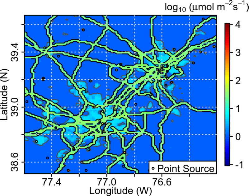
The actual emissions assumed here aim to represent three kinds of sources; area sources, transportation sources, and point sources. Two area sources are defined: urban emissions are based on the urban fraction computed from the MODIS-IGBP land cover, multiplied by 5 µmol m−2 s−1, with the remaining area assumed to emit 1 µmol m−2 s−1. Emissions from main roads are assumed to be 30 µmol m−2 s−1. Point source emissions are taken from the EPA GHG inventory, normalized by the area of one pixel (~ 1 km2). This inventory allows us to test the capabilities of the network for recovering a wide range of emissions (1–2400 µmol m−2 s−1) spatially distributed in a high resolution grid (Fig. 1). The simulated CO2 enhancements by using the inventory proposed here provided time series at the different stations with mean enhancements ranging from 3.5 to 8.5 ppm, a median from 1 to 4.4 ppm, and SD between 4 and 14 ppm, resembling the atmospheric variability observed in other urban settings (McKain et al., 2012; Lauvaux et al., 2016)
Fig. 1.
Assumed CO2 emissions inventory.
The diurnal cycle of photosynthesis and respiration significantly influences atmospheric mixing ratios of CO2, specifically in summer; photosynthesis draws down atmospheric CO2 during the daytime when fossil fuel CO2 is maximized. The presence of biogenic fluxes will, therefore, reduce the CO2 enhancements measured at the towers, increasing the relative importance of the uncertainties over the signal, thus significantly weakening the ability to estimate fossil fuel emissions in an urban environment. Although the a posteriori error covariance does not depend on the enhancements nor the a priori fluxes, the inclusion of biogenic fluxes will impact the values of the overall uncertainty reduction due to the fact that the a priori error covariance will account for the presence of those fluxes. This limitation will be important in determining the actual performance of a network configuration, especially in summer (July), but it will not have any impact on the comparison between network configurations.
3. Results and discussion
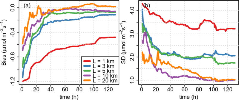
The correlation length used in the initial covariance Pb impacts observing system capabilities to constrain fluxes (Fig. 2). By using a correlation length equal to the grid resolution (1 km), the inversion system is challenged to constrain the fluxes. Most of the correction is applied nearby tower locations and is reflected in the bias and SD shown in Fig. 2. Larger correlation lengths positively impact retrieval quality, considerably reducing the bias and SD. However, as the correlation length is allowed to increase to 20 km, the SD increases, indicating that for this case, a correlation length of ~10 km seems appropriate (Fig. 2b). Similar performance in terms of the bias is also observed in Fig. 2a. This behavior seems to be in agreement with Lauvaux et al. (2012), who showed that including correlations that are too large can lead to an overly constrained system. Published values of the correlation length ranges from a few kilometers (< 10 km) to hundreds or thousands of kilometers (Mueller et al., 2008; Lauvaux et al., 2012, 2016). Typically, small values of the correlation length are associated with high-resolution studies conducted in a small domain with a relatively high density network, as seen in INFLUX (Lauvaux et al., 2016) and the case in this study, while large correlation length values are seen in low-resolution inversions in regional to global domains with sparse networks (Mueller et al., 2008).
Fig. 2.
The (a) bias and (b) standard deviation (SD) evolution of the CO2 flux retrieval for the urban land use in February (afternoon hours) by using 12 towers, a threshold of 25%, a model–data mismatch of 5 ppm, and five values of correlation length.
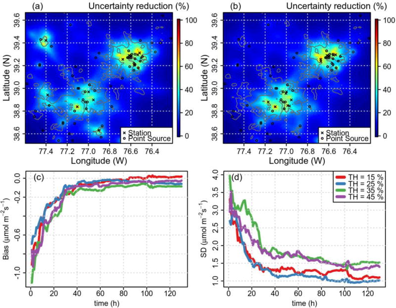
The user-defined threshold controls the compactness of the network, with higher threshold values resulting in a more compact network (Figs. 3a and b). The Baltimore area presents a denser network in all cases, probably due to higher variability in the meteorological conditions between stations due to the local effects produced by the proximity of Chesapeake Bay. The presence of more towers in the same area increases the uncertainty reduction in that specific area, leading to better local flux constraint. However, better performances in terms of total CO2 retrieved fluxes are achieved by using lower threshold values (Figs. 3c and d), due to the increased network spatial coverage. In addition, the mean uncertainty reduction in February for the urban land use is 29.5%, 30.5%, 30.2% and 28.2%, for threshold values of 15%, 25%, 35% and 45%, respectively. This indicates that too compact a network loses spatial coverage whilst too dispersed a network loses capability in constraining flux uncertainties. The selected threshold values covered the full range of urban contribution for the candidate towers. We do not expect the results to significantly improve the performances of the network in the threshold range of 25%–35%, due to the discrete nature of the possible candidates and the small differences between the values of uncertainty reduction shown for those two threshold values.
Fig. 3.
Uncertainty reduction using threshold values of (a) 15% and (b) 45%, and the (c) bias and (d) standard deviation (SD) evolution of the CO2 flux retrieval for the urban land use with four threshold values employed in the selection of the network for the month of February (afternoon hours) by using 12 towers, a correlation length 10 km, and a model–data mismatch of 5 ppm.
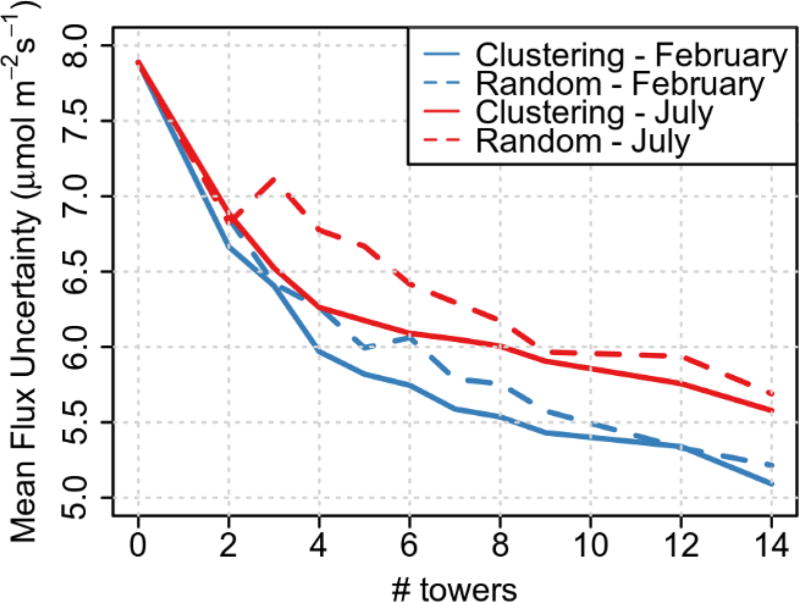
Figure 4 compares the mean CO2 flux estimated uncertainty for the urban area by using randomly selected networks and the proposed clustering approach. Both months, February and July, show a similar declining trend as the number of towers increases. However, July presents larger values of uncertainty, which is related to weaker sensitivities. The fact that the random method is significantly different from the clustering method shows that the latter is selecting observing locations in a smarter way. For instance, the random method could select two towers too close together and, therefore, the footprints would be highly overlapped, reducing the spatial coverage of the network. Another possibility is that the random method could pick locations too close to the edge of the urban area or with too little urban contribution, limiting the impact of that location on the inversion. From the results shown here, the proposed approach to select towers outperforms the random method. The benefits of the clustering approach are larger for July and for low tower numbers. Preselection of potential tower locations in the first stage improves the performances of the randomly selected networks, as there are only towers within the urban land use region available for selection, and therefore contributing to the networks’ measurement ability.
Fig. 4.
Mean CO2 flux estimated uncertainty for the urban area after a month of assimilation (afternoon hours only: 1700–2100 UTC) as a function of the number of towers employed using a randomly generated network (dashed lines) and the proposed clustering method (solid lines).
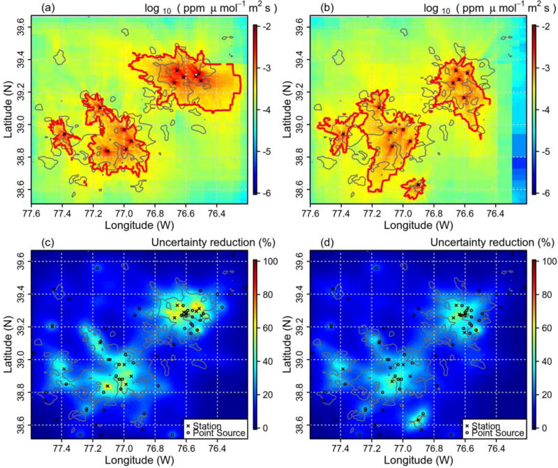
Figure 5 shows the average sensitivity and uncertainty reduction for the designed networks for the months of February and July using 12 towers, a 25% threshold (minimum urban CO2 contribution for a given tower candidate), and a 10 km correlation length. It is worth noting that during the summer (July), the excess of energy causes deeper boundary layers and enhanced mixing that reduces the tower sensitivity to the surface fluxes (footprints). Therefore, weaker sensitivities lead to smaller uncertainty reduction. Winter (February) is the opposite, showing larger values of sensitivities and uncertainty reduction. During spring and autumn, we can assume the situation will be something between the two, being that these two months are representative of the two extreme cases during the year. The tower distribution is also different for each month, caused by the different meteorological conditions. However, there are up to six coincident stations. In both cases, the networks show high sensitivity values for most of the MODIS-defined urban area. The average uncertainty reduction for the urban land use achieved by these networks is 31% and 25%, and the 95th percentile is 54% and 42% for February and July, respectively.
Fig. 5.
Average (a, b) sensitivity and (c, d) uncertainty reduction for the designed networks for the months of (a, c) February and (b, d) July, with 12 towers, a 25% threshold, and a 10 km correlation length. Red contours in the sensitivity plots correspond to 3.33×10⁻⁴ ppm (µmol m−2 s−1)−1.
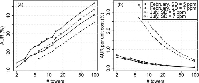
The average uncertainty reduction for urban land use increases as the number of towers increases, as expected (Fig. 6a). However, the uncertainty reduction is not additive and, therefore, the impact of adding towers decreases as the number of towers increases (Fig. 6b). The average uncertainty reduction per unit cost (ratio performance/cost) decreases proportionally to As a consequence, low numbers of towers would seem to be a more efficient selection. Nevertheless, in absolute numbers, more towers mean more uncertainty reduction, as well as more spatial coverage. Similar results were shown in Wu et al. (2016). On the other hand, by using low-accuracy sensors, the trend is conserved but shifted to lower values of average uncertainty reduction. For instance, 12 low-cost, low-accuracy sensors would perform the same as 7 high-accuracy sensors (Fig. 6a). However, assuming the high-accuracy sensors network would cost 10 times more than the low-accuracy sensors network (including the price of the sensors, installation and maintenance/calibration), the benefits of using the low cost sensors is rather clear. In this case, the average uncertainty reduction per unit cost (ratio performance/marginal cost) of a 96 low-cost sensors network is comparable to a network with 3–4 high-accuracy sensors (Fig. 6b). This fact impacts the capabilities of the network in reducing uncertainty and the spatial coverage.
Fig. 6.
The (a) average uncertainty reduction and (b) average uncertainty reduction per unit cost for the urban land use as a function of the number of towers after a month of assimilation (afternoon hours) for the months of February and July. The unit cost per tower is 10× for the case of 5 ppm and 1× for the case of 7 ppm.
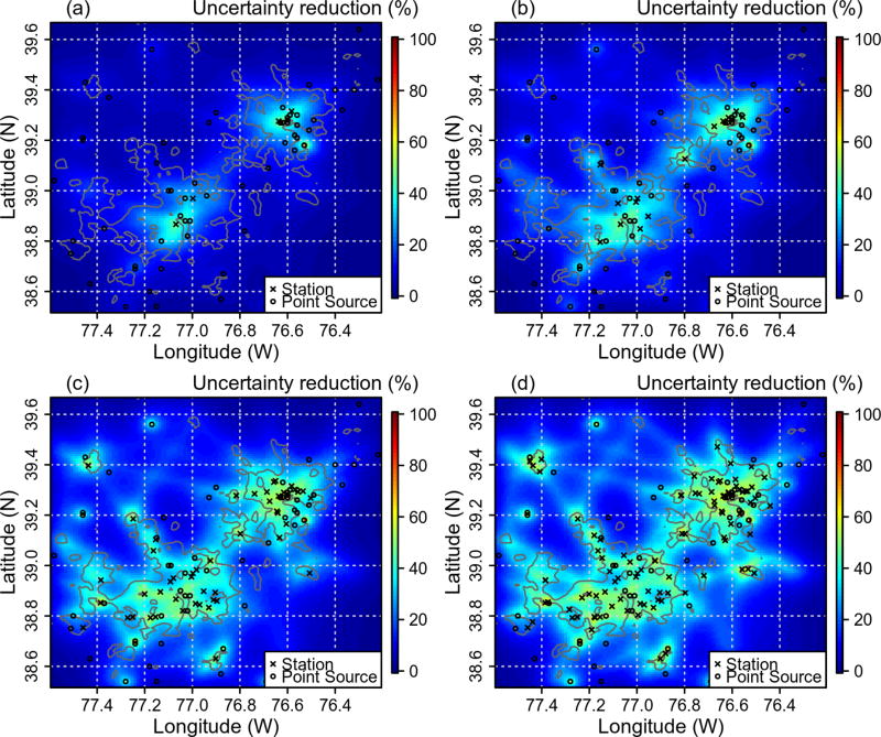
Despite the decreased efficiency per tower, adding new towers allows us to “see” areas nearby the added towers (Fig. 7). Thus, a network with too few stations (Fig. 7a), or one that is overly dense (Fig. 7b), would not be sufficient to constrain the fluxes for the whole urban area of Washington D.C. and Baltimore. Networks with a larger number of observing points (Figs. 7c and d) would cover the urban areas with considerably improved values of uncertainty reduction.
Fig. 7.
Uncertainty reduction for networks using (a) 4, (b) 14, (c) 48 and (d) 96 observing points, with a correlation length 10 km and model–data mismatch of 5 ppm for July (afternoon hours).
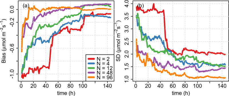
The addition of observing points also impacts the quality of the retrieved CO2 fluxes, as lower bias and SD are obtained by using a larger number of towers (Fig. 8). In addition, the convergence to the true values is faster with a large number of towers, reducing the response time of the filter (Fig. 8a). Thus, by using 12 towers, the spin-up time of the filter is in the order of 100 h, 20 days, if we use just 5 h during the afternoon hours. On the other hand, by using 96 towers, the spin-up time of the filter is reduced to just 10 h, 2 days. Reducing the spin-up time of the filter directly impacts the analysis system’s ability to constrain time-dependent fluxes to shorter time scales.
Fig. 8.
The (a) bias and (b) standard deviation (SD) evolution of the CO2 flux retrieval for the urban land use in July (afternoon hours) by using 2, 4, 12, 48 and 96 observing points, with a correlation length of 10 km and model–data mismatch of 5 ppm.
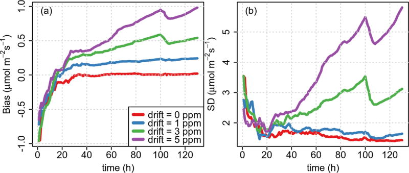
Sensor drift is a bias in nature. Such drift disrupts the Gaussian assumptions, therefore biasing the retrieved fluxes. Low drift (1 ppm) results in small bias, slowly increasing with time. In addition, the SD is also low and comparable to the case with no drift (Fig. 9). On the other hand, larger drifts (3 and 5 ppm) result in bias and SD dramatically increasing with time as the drift increases. This fact makes it unacceptable to perform inversions and periodic calibrations would be required in order to minimize the impact of the drift. From these results, an optimum calibration period for large drifts would be in the order of half of the spin-up time of the filter (~ 20 h in the case of February, with 24 observing points).
Fig. 9.
The (a) bias and (b) standard deviation (SD) evolution of the CO2 flux retrieval for the urban land use in February (afternoon hours) by using 24 observing points, with a correlation length of 10 km, model–data mismatch of 5 ppm, and 0, 1, 3 and 5 ppm total drift.
4. Conclusions
High-resolution simulations along with clustering analysis were used to design a network of surface stations for the area of Washington D.C./Baltimore. Thereafter, a Kalman filter within an OSSE was employed to evaluate the performances of different networks consisting of different number of towers and where the location of these towers varied. Additionally, we explored the possibility of using a very high density network of low-cost, low-accuracy sensors characterized by larger uncertainties and drift over time.
The results show that overly compact networks lose spatial coverage, whilst overly spread-out networks lose capability in constraining uncertainties in the fluxes. July presents weaker sensitivities and, therefore, lower uncertainty reduction. The tower distribution is also different for each season, caused by the different meteorological conditions. However, there are up to six coincident stations. In both cases, the networks show high sensitivity values and uncertainty reduction for most of the urban land use.
The average uncertainty reduction for the urban land use increases as the number of towers increases. However, the uncertainty reduction is not additive and, therefore, the impact of adding towers decreases as the number of towers increases. By using low-accuracy sensors, the trend is conserved but shifted to lower values of average uncertainty reduction. For instance, 12 low-cost, low-accuracy sensors would perform the same as 7 high-accuracy sensors. Nevertheless, the benefits of using low-cost sensors is rather clear. In this case, the average uncertainty reduction per unit cost (ratio performance/marginal cost) of a 96 low-cost sensors network is comparable to a network with 3–4 high-accuracy sensors. This fact impacts the capability of the network in reducing uncertainty and the spatial coverage. In addition, the convergence to the true values is faster with a large number of towers, reducing the response time of the filter, which directly impacts our ability to constrain time-dependent fluxes at shorter time scales.
The drift is a bias in nature, which is added to the observations, therefore biasing the retrieved fluxes. Low drift results in bias and SD comparable to the case with no drift. On the other hand, larger drifts results in bias and SD dramatically increasing with time as the drift increases. This fact makes it unacceptable to perform inversions, and periodic calibrations would be required in order to minimize the impact of the drift.
Acknowledgments
The authors would like to thank Dr. Adam PINTAR of the National Institute of Standards and Technology for his insightful comments on the covariance model employed in this work. Funding was provided by the NIST Greenhouse Gas and Climate Science Measurements program. Any opinions, findings and conclusions or recommendations expressed in this material are those of the authors and do not necessarily reflect the views of NIST.
References
- Bréon FM, et al. An attempt at estimating Paris area CO2 emissions from atmospheric concentration measurements. Atmos. Chem. Phys. 2015;15:1707–1724. [Google Scholar]
- Brioude J, et al. A new inversion method to calculate emission inventories without a prior at mesoscale: Application to the anthropogenic CO2 emission from Houston, Texas. J. Geophys. Res. 2012;117(D5):D05312. doi: 10.1029/2011JD016918. [DOI] [Google Scholar]
- Cambaliza MOL, et al. Assessment of uncertainties of an aircraft-based mass balance approach for quantifying urban greenhouse gas emissions. Atmos. Chem. Phys. 2014;14:9029–9050. [Google Scholar]
- Coniglio MC, Correia J, Marsh PT, Kong FY. Verification of convection-allowing WRF model forecasts of the planetary boundary layer using sounding observations. Wea. Forecasting. 2013;28:842–862. [Google Scholar]
- Duren RM, Miller CE. Measuring the carbon emissions of megacities. Nature Clim Change. 2012;2:560–562. [Google Scholar]
- Forgy EW. Cluster analysis of multivariate data: Efficiency versus interpretability of classifications. Biometrics. 1965;21:768–769. [Google Scholar]
- Gerbig C, Lin JC, Wofsy SC, Daube BC, Andrews AE, Stephens BB, Bakwin PS, Grainger CA. Toward constraining regional-scale fluxes of CO2 with atmospheric observations over a continent: 2. Analysis of COBRA data using a receptor-oriented framework. J. Geophys. Res. 2003;108(D24):4757. [Google Scholar]
- Hartigan JA, Wong MA. Algorithm AS 136: A K-means clustering algorithm. Applied Statistics. 1979;28:100–108. [Google Scholar]
- Hungershoefer K, Breon F-M, Peylin P, Chevallier F, Rayner P, Klonecki A, Houweling S, Marshall J. Evaluation of various observing systems for the global monitoring of CO2 surface fluxes. Atmos. Chem. Phys. 2010;10:10 503–10 520. [Google Scholar]
- IPCC. Climate Change 2013: The Physical Science Basis. In: Stocker, et al., editors. Working Group I Contribution to the Fifth Assessment Report of the Intergovernmental Panel on Climate Change. Cambridge University Press; Cambridge: 2013. p. 1552. [Google Scholar]
- Janjić ZI. The step-mountain Eta coordinate model: Further developments of the convection, viscous sublayer, and turbulence closure schemes. Mon. Wea. Rev. 1994;122:927–945. [Google Scholar]
- Kain JS. The Kain-Fritsch convective parameterization: An update. J. Appl. Meteor. 2004;43:170–181. [Google Scholar]
- Kort EA, Angevine WM, Duren R, Miller CE. Surface observations for monitoring urban fossil fuel CO2 emissions: Minimum site location requirements for the Los Angeles Megacity. J. Geophys. Res. 2013;118:1577–1584. [Google Scholar]
- Lauvaux T, Schuh AE, Bocquet M, Wu L, Richardson S, Miles N, Davis KJ. Network design for mesoscale inversions of CO2 sources and sinks. Tellus B. 2012;64:17980. [Google Scholar]
- Lauvaux T, et al. High-resolution atmospheric inversion of urban CO2 emissions during the dormant season of the Indianapolis Flux Experiment (INFLUX) J. Geophys. Res. 2016;121:5213–5236. doi: 10.1002/2015JD024473. [DOI] [PMC free article] [PubMed] [Google Scholar]
- Lin JC, Gerbig C, Wofsy SC, Andrews AE, Daube BC, Davis KJ, Grainger CA. A near-field tool for simulating the upstream influence of atmospheric observations: The Stochastic Time-Inverted Lagrangian Transport (STILT) model. J. Geophys. Res. 2003;108(D16):4493. [Google Scholar]
- Lorenc AC. Analysis methods for numerical weather prediction. Quart. J. Roy. Meteor. Soc. 1986;112:1177–1194. [Google Scholar]
- Loveland TR, Belward AS. The IGBP-DIS global 1km land cover data set, DISCover: First results. Int. J. Remote Sens. 1997;18:3289–3295. [Google Scholar]
- McKain K, Wofsy SC, Nehrkorn T, Eluszkiewicz J, Ehleringer JR, Stephens BB. Assessment of ground-based atmospheric observations for verification of greenhouse gas emissions from an urban region. Proceedings of the National Academy of Sciences of the United States of America. 2012;109:8423–8428. doi: 10.1073/pnas.1116645109. [DOI] [PMC free article] [PubMed] [Google Scholar]
- Mellor GL, Yamada T. Development of a turbulence closure model for geophysical fluid problems. Rev. Geophys. 1982;20:851–875. [Google Scholar]
- Mlawer EJ, Taubman SJ, Brown PD, Iacono MJ, Clough SA. Radiative transfer for inhomogeneous atmospheres: RRTM, a validated correlated-k model for the longwave. J. Geophys. Res. 1997;102(D14):16 663–16 682. [Google Scholar]
- Mueller KL, Gourdji SM, Michalak AM. Global monthly averaged CO2 fluxes recovered using a geostatistical inverse modeling approach: 1. Results using atmospheric measurements. J. Geophys. Res. 2008;113(D21):D21114. [Google Scholar]
- Nakanishi M, Niino H. An improved Mellor-Yamada Level-3 model: Its numerical stability and application to a regional prediction of advection fog. Bound.-Layer Meteor. 2006;119:397–407. [Google Scholar]
- Nehrkorn T, Eluszkiewicz J, Wofsy SC, Lin JC, Gerbig C, Longo M, Freitas S. Coupled weather research and forecasting-stochastic time-inverted Lagrangian transport (WRF-STILT) model. Meteor. Atmos. Phys. 2010;107:51–64. [Google Scholar]
- Patil MN, Waghmare RT, Halder S, Dharmaraj T. Performance of Noah land surface model over the tropical semi-arid conditions in western India. Atmospheric Research. 2011;99:85–96. [Google Scholar]
- Rosenzweig C, Solecki W, Hammer SA, Mehrotra S. Cities lead the way in climate-change action. Nature. 2010;467:909–911. doi: 10.1038/467909a. [DOI] [PubMed] [Google Scholar]
- Ruiz-Arias JA, Dudhia J, Santos-Alamillos FJ, Pozo-Vázquez D. Surface clear-sky shortwave radiative closure intercomparisons in the Weather Research and Forecasting model. J. Geophys. Res. 2013;118:9901–9913. [Google Scholar]
- Shiga YP, Michalak AM, Randolph Kawa S, Engelen RJ. In-situ CO2 monitoring network evaluation and design: A criterion based on atmospheric CO2 variability. J. Geophys. Res. 2013;118:2007–2018. [Google Scholar]
- Skamarock WC, et al. A description of the advanced research WRF version 3. NCAR Technical Note NCAR/TN-475+STR 2008 [Google Scholar]
- Strahler A, Muchoney D, Borak J, Friedl M, Gopal S, Lambin E, Moody A. MODIS land cover product algorithm theoretical basis document (ATBD) version 5.0: MODIS land cover and land-cover change. USGS, NASA; 1999. [Available online from http://modis.gsfc.nasa.gov/data/atbd/atbd_mod12.pdf] [Google Scholar]
- Thompson G, Rasmussen RM, Manning K. Explicit forecasts of winter precipitation using an improved bulk microphysics scheme. Part I: Description and sensitivity analysis. Mon. Wea. Rev. 2004;132:519–542. [Google Scholar]
- Turnbull JC, et al. Toward quantification and source sector identification of fossil fuel CO2 emissions from an urban area: Results from the INFLUX experiment. J. Geophys. Res. 2015;120:292–312. [Google Scholar]
- Wu L, Broquet G, Ciais P, Bellassen V, Vogel F, Chevallier F, Xueref-Remy I, Wang YL. What would dense atmospheric observation networks bring to the quantification of city CO2 emissions? Atmospheric Chemistry and Physics. 2016;16:7743–7771. [Google Scholar]
- Ziehn T, Nickless A, Rayner PJ, Law RM, Roff G, Fraser P. Greenhouse gas network design using backward Lagrangian particle dispersion modelling-Part 1: Methodology and Australian test case. Atmospheric Chemistry and Physics. 2014;14:9363–9378. [Google Scholar]


