Conceptual designs of conduction cooled MgB2 magnets for 1.5 and 3.0T full body MRI systems

Abstract

Conceptual designs of 1.5 and 3.0 T full-body magnetic resonance imaging (MRI) magnets using conduction cooled MgB₂ superconductor are presented. The sizes, locations, and number of turns in the eight coil bundles are determined using optimization methods that minimize the amount of superconducting wire and produce magnetic fields with an inhomogeneity of less than 10 ppm over a 45 cm diameter spherical volume. MgB₂ superconducting wire is assessed in terms of the transport, thermal, and mechanical properties for these magnet designs. Careful calculations of the normal zone propagation velocity and minimum quench energies provide support for the necessity of active quench protection instead of passive protection for medium temperature superconductors such as MgB₂. A new ‘active’ protection scheme for medium T_c based MRI magnets is presented and simulations demonstrate that the magnet can be protected. Recent progress on persistent joints for multifilamentary MgB₂ wire is presented. Finite difference calculations of the quench propagation and temperature rise during a quench conclude that active intervention is needed to reduce the temperature rise in the coil bundles and prevent damage to the superconductor. Comprehensive multiphysics and multiscale analytical and finite element analysis of the mechanical stress and strain in the MgB₂ wire and epoxy for these designs are presented for the first time. From mechanical and thermal analysis of our designs we conclude there would be no damage to such a magnet during the manufacturing or operating stages, and that the magnet would survive various quench scenarios. This comprehensive set of magnet design considerations and analyses demonstrate the overall viability of 1.5 and 3.0 T MgB₂ magnet designs.

1. Introduction

Magnetic resonance imaging (MRI) is an indispensable modality for medical diagnostics and treatment monitoring with approximately 35 000 MRI systems installed worldwide and a growing market expected to reach $7.4 billion per year [1, 2]. Within the MRI market, the most common full body clinical systems operate with main magnetic field strengths of 1.5 T or 3.0 T, rely on the use of liquid helium (LHe) to reach the 4.2 K operating temperature, and generate the leading market for superconducting wire. For most clinical MRI magnets in use today, the superconducting material of choice is niobium titanium (NbTi) with a critical temperature, T_c, of 9K [3]. To maximize the current capacity of the NbTi wires (i.e. critical current), and to enable operation in persistent current mode, the superconducting magnets are cooled to temperatures well below the critical temperature 9 K. Typically, NbTi based MRI magnets are operated at temperature of 4.2 K by completely submersing the magnet coils in a LHe bath. Over the lifetime of a MRI system, such a magnet consumes approximately 1500–2000 l of LHe; first for the initial cool down and testing at the factory, and similar amounts later for magnet quenches in the field [1]. Given the size of the MRI market, and the reliance on LHe, it is not surprising that 25% of the world-wide demand for LHe comes from the MRI industry [4, 5].

In the last few years the price of LHe has increased substantially, and further price increases are expected this decade as the growth in demand is projected to outpace the growth in supply [2]. The higher cost of LHe will increase the cost of siting and maintaining LHe cooled MRI systems. Additionally, the limited availability of LHe in remote areas and third-world countries adversely affects patient access to the 1.5 and 3.0 T MRI systems preferred by radiologists. In lieu of these systems, which rely on LHe for operations, low-field (0.2–0.5 T) MRI systems with permanent magnets are deployed since they do not require LHe for operations. Unfortunately, this impacts most of the Earth’s seven billion inhabitants. Recently, researchers at Los Alamos National Laboratories have developed and are testing for field deployment an MRI utilizing superconducting quantum interference devices (SQUIDS) and the Earth’s magnetic field [6, 7]. However, if the higher field MRI, a standard in the developed world, could be made LHe free, then these higher resolution diagnostic tools would be more available for deployment in third-world countries and remote areas. Consequently, the MRI scientific community has been actively exploring and developing suitable alternatives to LHe bath-cooled MRI main magnets [5].

One alternative to a ‘wet’ magnet, which is cooled using a bath of LHe, is a conduction cooled ‘dry’ magnet with a two stage cryocooler to provide refrigeration. Only 1–3 l of LHe would be required to operate the cryocooler. The magnet coils would be thermally connected to the cryocooler cold head using flexible thermally conducting straps (such as copper), and subsequently cooled via conduction to the cold head [7]. With a T_c substantially higher than NbTi, superconducting materials such as Nb₃Sn (T_c = 17 K), MgB₂ (T_c = 39 K) [8], YBCO (T_c = 93 K) [9], BSCCO (T_c = 108 K) [10], and Bi-2223 (T_c = 90–95 K) [11] are all potential candidates for conduction cooled magnet designs. Among the HTS options for superconducting magnets, MgB₂ has the lowest T_c. The advantage a higher T_c material is the increased range of operating temperature which facilitates the design of conduction cooled magnets by allowing larger temperature gradients in the coil windings (compared to NbTi) during operation. Consequently the dependence on LHe can be reduced or even eliminated.

MgB₂ is of interest because it is affordable, has a moderately high T_c, is available in wire form, and can be formed into persistent joints [12–14]. There has been a great deal of research on the properties of MgB₂ conductors to date, including the assessment of different types of the performance of various monofilament [15] and multifilament [16] wire configurations, as well as the development of conductors with the proper strand architecture and mechanical properties for applications.

Concurrent with the development in MgB₂ wire, the viability of MgB₂ based magnets has been an active area of research. A 3.0 T, 250 mm bore magnet with MgB₂ has been built and operated [17]. Progress on the development of low cost, LHe free magnets has been reported in [18] and 0.6 T, 650 mm bore, solid nitrogen cooled MgB₂ demonstration coil was described in [19]. MRI magnet designs using MgB₂ and operating at 10 K or higher have been investigated [15, 20–22], and a test coil by Iwasa, has been built and intentionally quench tested [20]. Monofilamentary MgB₂ wires have been used to develop coils for 0.5 T, 240 mm diameter bore magnets [15]. Work on conduction cooled NbTi based MRI systems has also been pursued [18].

In the commercial market, the MR Open (Paramed Medical Systems) MRI contains a 0.5 T, LHe free MgB₂ magnet. Since the magnet uses an iron core, and operates in driven current more, such a magnet design does not easily translate into a suitable magnets for 1.5 and 3.0 T MRI systems. In addition to the stronger field, the magnets for the 1.5 and 3.0 T MRI systems are operated in persistent current mode, (which requires the development of a persistent switch), and the magnets must be iron free to maintain the weight limits at MRI sites. Since the magnet operates in driven current mode, a dump resistor may be used as part of the quench protection. For a persistent current mode magnet, it is necessary to use more sophisticated quench protection system which does not relay on dump resistor.

Although a much broader interest exists for super-conducting magnets and MRI systems, the focus of this work is the conceptual design of a 1.5 T or 3.0 T, conduction cooled, full body, MRI system using MgB₂ wire. This conceptual design has been a topic of research interest and much has been accomplished in the development of MgB₂ wire, quench propagation characteristics, prototype coils, experimental testing, the quenching of coil bundles, and persistent joints. However, there has been no presentation of a complete conceptual designs for 1.5 and 3 T MgB₂ MRI magnets.

This work provides conceptual design of magnets with MgB₂ wire for 1.5 and 3.0 T full-body MRI systems. The coil geometry is determined using optimization techniques and the measured transport properties of MgB₂ wire. Finite element analysis (FEA) of the mechanical stress and strain in the MgB₂ wire and epoxy for these designs are presented for the first time. Quench simulations of this geometry are performed to understand the temperature rise and profile in the coil bundles during a quench, and it is concluded that active intervention is needed to reduce the temperature rise in the coil bundles and prevent damage to the superconductor. One possible active protection system is presented and shown to be effective in protecting the magnet from damage during a quench. Recent progress on persistent joints for multifilament MgB₂ wire is also presented. This work, which combines a comprehensive set of magnet design considerations and analysis with recent results on conductors and persistent joints demonstrates the overall viability of 1.5 and 3.0 T MgB₂ magnet designs.

1.1. 1.5 and 3.0 T MgB₂ MRI magnet requirements

The specifications and design choices for MRI magnets, such as bore size and magnet length, can vary between manufactures and magnet designers. In this section the magnet criteria and design choices for the magnets developed in the paper are listed.

1.1.1. Bore size

The coil windings in the magnet design have a minimum inside diameter of 95 cm which allows for a 60 cm warm bore, and leaves space for the coil formers, vacuum vessel, gradient coils, and RF coils.

1.1.2. Bore length

The end-to-end length of the magnet windings is 1.55 m and 1.82 m for the 1.5 T and 3.0 T designs, respectively. The total bore lengths will be approximately 10% larger then these lengths once the cryogenic cooling and vacuum vessel are added. Magnets with shorter length are desired [23], but the performance of the MgB₂ wire chosen in this work limits the length of the magnet. Shorter magnet designs will be enabled with improved MgB₂ performance expected in the future.

1.1.3. Field uniformity

Image quality, resolution, off-resonance frequency resolution are determined by the uniformity of the magnetic field within the imaging region. The magnet designs are based on achieving magnetic field deviations of 10 ppm or less over a 45 cm diameter spherical volume (DSV).

1.1.4. Shim coils

Shim coils are an essential part of a MRI system and are needed to correct main field inhomogeneities of ~1000 ppm related to inaccuracies in the coil positions due to manufacturing tolerances. The magnet designs in this paper do not specify a shim coils system, but the shim coils can be implemented by: (1) using superconducting shims and incorporating them within the cold mass, or (2) using resistive shims placed within the warm bore (as is now employed in some NbTi designs).

1.1.5. Stray field

For safety reasons, the magnitude of the stray magnetic field outside of the MRI imaging room must be less than 5 Gauss (0.5mT) [24]. With a shielding coil included in the design, the 5 Gauss line extends no further than 3m from the center of the scanner in the 1.5 T magnet (or 4 m for the 3.0 T magnet).

1.1.6. Field temporal stability

The magnetic field strength cannot drift more than 0.1 ppm hr⁻¹. This level of temporal stability is required to preserve image quality during a scan, and on a longer time frame to reduce the need for magnet recharging [24].

1.1.7. Optimal location of coil bundles

The number, size, and location of the magnet wire bundles are determined from an optimization technique [8] which minimizes the amount of superconducting wire while still meeting the previously listed constraints on the magnetic field profile.

1.1.8. Persistent current mode

The designs assume the magnets operate in persistent current mode (PCM) which provides long term stability of the magnetic field provided the n-value of the superconducting wire is greater than ~30, and the magnet is operated with a I_op/I_c ratio less than ~0.7 [25].

1.1.9. Persistent current switch

It is not possible to charge a superconducting wire loop (i.e. magnet) without a persistent current switch (PCS). While charging the magnet, the PCS is heated above the critical temperature to create electrical resistance within the PCS. When charging is complete, the PCS is cooled to the magnet operating temperature and becomes superconducting.

1.1.10. Persistent joints

Operating in persistent current mode, with the strict requirements on the field stability, is only possible if the joints connecting two wire ends have a resistance across the joint of less than 10⁻¹² Ω [24].

1.1.11. React-and-wind wire

The type of MgB₂ wire will be react-and-wind. In this case, care must be taken at all steps of manufacturing and operation to limit the strain to less than the maximum strain of 0.4%. The design goal is to provide a safety factor and limit the maximum strain during operation to less than 0.2% for MgB₂ reacted wire.

1.1.12. Conduction cooled

The magnet is designed for conduction cooling. A two stage cryocooler provides the cooling of the coil bundles via conduction through copper cooling rings and straps. Other methods for magnet cooling, such as a LHe bath, or a reduced helium approach, might be possible but are not considered here.

1.1.13. Operating temperature

The temperature of the warmest regions of the MgB₂ magnet will be 10 K. Higher temperatures would reduce the critical current in the MgB₂ wire, especially in regions with the highest magnetic field on the wire.

1.1.14. Reliability

Reliability of the MRI system is crucial for commercial success. Although myriads of considerations fall under this category, the focus here is on the protection of magnet during a quench.

1.1.15. Quench detection and active protection

It is generally accepted that high temperature superconducting (HTS) magnets operating in persistent mode cannot be passively protected [25]. The magnet designs therefore include an active quench protection system that relies on an external power source, and is triggered via a quench detection system.

1.1.16. Strain limit on MgB₂ wire

The mechanical stress and strain developed in the magnet must remain below material failure limits, and one of the most limiting factors is the strain limit on the superconducting MgB₂. The precise strain limit on the MgB₂ wire depends upon its composition and manufacturing technique. The design limit is based on published experimental results [26], thermal expansion models of the wire, and a design safety factor. These limits are explained further in section 7.3, but here we quickly mention that a strain limit of 0.2% is well below the 0.4% maximum to provide a large safety margin for the strain limit on the on the MgB₂ wires.

2. MgB₂ superconductor wire for MRI

With the desire to move away from helium bath cooling, the advantage of MgB₂ wire for 1.5 and 3.0 T full body MRI magnets is the higher operating temperature of the superconductor. (The same advantage also applies to other medical superconducting magnets such as image guided MRIs, and gantry magnets for radiation therapy). For these applications, the magnets must operate in a persistent current mode, which means the power loss allowed for the superconductor current is zero. Zero power loss is achieved by cooling the superconductor below the 39 K transition temperature of MgB₂, and keeping the magnet current below the critical current value, I_c, at the desired magnetic field B and temperature T.

Typically, the most economical magnet design will operate at a temperature that minimizes the combined cost of the wire and the cooling system. In the case of large conduction cooled MgB₂ MRI magnets as discussed in this paper, a temperature range of 4–10 K is found to be practical, as compared to the 4–5 K temperature range of NbTi MRI magnets in a LHe bath. For large NbTi MRI magnets, it is difficult to maintain the temperature within the 4–5 K range using conduction cooling techniques. Operating NbTi at higher temperatures would require operating at a lower percentage of critical current to prevent power loss in the superconductor, which translates to a considerable increase in the amount of NbTi wire to maintain the same strength magnetic field. In the case of MgB₂, however, the larger operating temperature range facilitates the design of a conduction cooled magnet.

2.1. Status of commercial MgB₂ superconductor wire

Present commercial MgB₂ superconductor wires are manufactured by either the in situ or ex situ methods. In-situ implies that the MgB₂ is formed during heat treatment from elemental magnesium and boron (Mg + B) after the wire has been manufactured and drawn down to its final size. With the ex situ method, the MgB₂ powder is manufactured from elemental Mg + B powder before it is placed in the wire, and at the end of the manufacturing process, the wire is sintered to connect the MgB₂ particles. The sintering temperature is typically higher than the temperature used initially to form MgB₂. Presently, in situ MgB₂ wires have resulted in higher critical current densities (J_c) than ex situ wires for the highest in-field performance.

The cross section of a typical rectangular shaped, in situ MgB₂ wire considered for conduction cooled MRI magnet (figure 1) shows the internal components: MgB₂, niobium (Nb) barrier, Monel (Ni–Cu) for wire drawing and copper (Cu) for magnet protection. In superconducting MRI magnets, the copper in the wire helps limit the local temperature rise during a quench by reducing the resistance of the wire, and by providing additional heat capacity to absorb the energy from resistive heating during the quench. One of the most important factors to minimize the amount and cost for an MRI magnet, when using MgB₂ wire, such as full body 1.5 T or 3.0 T MRI magnet, is to minimize the amount of copper and Monel in the wire, yet keep enough Cu to protect the magnet during a quench. The engineering current density, J_e, is maximized when the copper and Monel content are minimal, which allows for more compact magnet designs and thus lowers the total cost of the conductor in the magnet. However, the temperature rise is lower during a quench when more copper is present to act as an electrical short (and heat sink). Thus, for a given a fixed wire cross sectional area, a trade-off exists between the percentage of superconductor (and the resulting critical current, I_c) and the percentage of copper in the wire strand. For the MRI magnet designs in this paper, the copper to superconductor ratio, Cu:SC, should be optimized subject to constraints on manufacturing techniques, balancing the needs for maximizing J_e but also allowing for quench protection. Section 7.1 discusses this in more detail.

Figure 1.

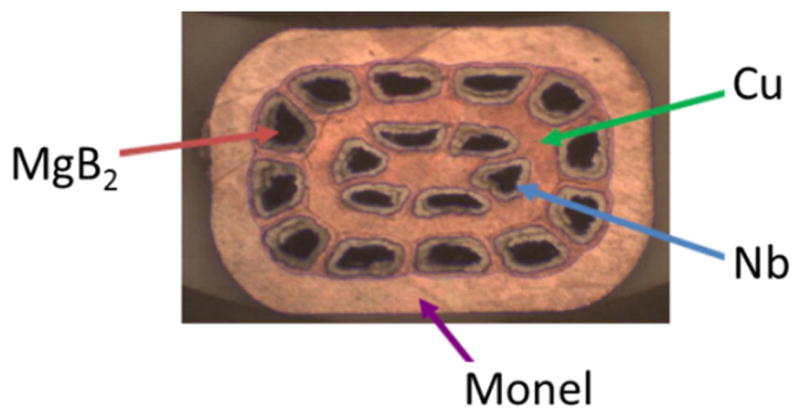
A cross section of a 1.5 mm × 1.0 mm rectangular MgB₂ wire for MRI applications. The example shown has 18 superconducting filaments with a Cu:SC ratio of 2.7:1.

The critical current density, J_c, of the superconducting wire is one measure of wire performance, and has a strong impact on the length of superconducting wire needed to build a magnet. The critical current density as a function of temperature and magnetic field strength on wire has been experimentally determined for a commercially available wire [27]. This particular MgB₂ wire is manufactured using an in situ technique and is generally referred to as 1st generation wire. Experimental measurements of the critical current densities and index values (n-value) of this wire as a function of magnetic field strength are shown in figure 2 for a 0.83 mm diameter wire with superconductor fraction of 12% MgB_2. The n-value of a wire is a second important quality factor for the conductor, and typically must be greater than 25 at the B and T in the winding in order to allow for persistent mode operation at acceptably high levels of I_op/I_c to allow viable system designs. If we require, for example, 200 A or more for I_c, and n values of 25 or greater, we can see from figure 2 that MgB₂ in principle should be viable for 1.5 and 3 T designs, a point which we delve deeply into in the present paper.

Figure 2.

(a) (left) I_c of a round, 0.83 mm diameter wire with 12% MgB₂, and (right) J_c (I_c normalized to MgB₂ cross sectional area) at various magnetic field strengths and temperatures, (b) index value, n, (slope of log–log plot near I_c) versus B and T for the same wire. (Wire HTR 1654 [27]).

The sample for these measurements were made with carbon-doped SMI boron. Short samples were heat treated at it 675 °C for 20 min. Additional information for the wire is provided in table 1.

Table 1.

Specifications of MgB₂ strand HTR 1654.

Fil. no.	Barrier	Mono sheath	Multi sheath	Powder material	B source	Mg:B	OD	% powder
6	Nb	Cu	Monel	MgB2_2%C	SMI	1:2	0.834	11.7

These wires are available in lengths up to 10 km with braided insulation for coil winding and epoxy impregnation and have been used to make both ‘wind and react’ and ‘react and wind’ coils. Reacted wire has been wound into coils using wet lay with epoxy and vacuum impregnated coils, and wires with the properties of these in situ MgB₂ wires are being used to design 1.5 and 3.0 T full body MRI magnets as well as specialty MRI magnets such as image-guided MRI background magnets.

2.2. Future improvements for MgB₂ wires

The critical current density of MgB₂ superconductor wire can be increased by using a technique in which the magnesium diffuses magnesium diffuses into boron powder. Referred to a 2nd generation wire, it has been fabricated in short lengths using both monofilament and multifilament wire [28]. A comparison between critical current densities of 1st generation in situ MgB₂ wire and 2nd generation internal diffusion MgB₂ wire (figure 3) shows improvements at 4.2 K by factors of 2–10 depending on the strength of the field on wire. For magnetic field strengths of 4 T on the wire, typical for a 1.5 T full body magnet design, the J_c is increased by a factor of 3.5. For magnetic field strengths of 6 T on wire, typical for a 3.0 T full body magnet design, the J_c is increased by a factor of 4. Development is in progress to manufacture 2nd generation wire in the lengths needed for full body MRI magnets. These types of improvements contribute to higher performance, thus more easily enable the commercialization of full body conduction cooled 1.5 and 3.0 T MRI background magnets using MgB₂ wires.

Figure 3.

(a) A comparison of critical current density, J_c, versus magnetic field strength at 4.2 K for 1st generation in situ MgB₂ wire (HTR 1654) and AIMI 2nd generation wire (HTR 2281) [28]. (b) Measurements of n-value for a 2nd generation HTR 2281 [28] wire versus magnetic field at various temperatures.

The magnet designs in this paper, using 1st generation MgB₂, are longer than some of the NbTi magnets used in MRI systems. The longer designs stems from the performance of the 1st generation wire and its demonstrated critical current density. In a commercial market, the size of the MRI warm bore is important for patient access and comfort, and to reduce the feeling of claustrophobia. With the projected improvements of 2nd generation MgB₂ wire, the current density in the wire could be increased, and facilitate the design of MRI magnets that are shorter and similar in length to some of the NbTi magnets used today. This topic is discussed further in section 3.6.

2.3. Other potential superconductors for conduction cooled 1.5 and 3.0 T MRIs

Besides NbTi and MgB₂, other superconducting wire manufactured in lengths long enough for magnet demonstrations have been based on Nb₃Sn, BSCCO 2212, BSCCO 2223, and (RE)BCO superconductors. Each of these superconductors could in principle be considered for conduction cooled 1.5 and 3.0 T full body MRIs. They have higher operating temperatures than NbTi superconductors and could be operated in the 4–10 K temperature range to enable full conduction cooled MRI magnets. However, each have disadvantages compared to MgB₂ superconductors. BSCCO 2212, BSCCO 2223, and (RE)BCO have higher operating temperature but have two difficulties: (1) the development of persistent joints at the level of quality needed for MRI persistent coils and joints; and (2) the price performance ($/kAm) in the 4–10 K, 4–6 T range. The present $/kAm for all three is high and is expected to remain high compared to NbTi and projected MgB₂ wires. However, Nb₃Sn superconductor wire could be considered for conduction cooled MRI full body magnets for 3 and 7 T full body MRIs. MRI quality persistent joints have been demonstrated with Nb₃Sn and much progress has been made during the last 10 years in improving the J_c of Nb₃Sn wires. Large volumes of Nb₃Sn superconductor wires have been made for the International Fusion Program (ITER), which have critical current densities of 800–1000 A mm⁻² at 12 T and 4.2 K [29].

Recently, further improved Nb₃Sn superconductor wire with current densities in the 2000–2500 A mm⁻² at 12 T and 4.2 K are being manufactured in volume for high energy physics accelerators. There is a potential to raise the critical current density J_c of Nb₃Sn even higher, to over 10 000 A mm⁻² at 12 T–4.2 K, with a new artificial pinning (fine grain) approach [30, 31]. The J_c at field of Nb₃Sn at 8 K is around half that at 4.2 K. Since the critical current density J_c of Nb₃Sn at 8 K is about half the value at 4.2 K, conduction cooled Nb₃Sn magnets operating at 4–8 K could be designed with magnetic fields of 10 T on wire for 7 T MRI systems or magnetic fields of 6 T on wire for 3 T MRI systems with less $/kAm cost of NbTi wire. Much needs to be proven and developed for these artificial pinning center (APC) Nb₃Sn wires, but the potential for Nb₃Sn for conduction cooled Nb₃Sn MRI large background magnets in the 3–7 T range exists.

3. Magnetic design

MRI magnet designs are dominated by the need to maximize the field homogeneity inside the DSV, and minimize the strength of the stray field, using a reasonable length and radius for the magnet windings. Typically a number of individual coil bundles, electrically connected in series, are used to generate the magnetic field. In this work, the size and location if the individual coils are determined using an optimization method for shielded magnet designs, which has been discussed in detail in previous publications [8, 32]. The resulting coil geometry is used to calculate the magnet field within the bundles and the ratio of operating to critical current, I_op/I_c, in order to verify the design.

For the particular 1.5 and 3 T MRI magnet designs in this work, the uniformity of the magnetic field was set to deviate by less than 10 ppm over a 45 cm DSV. In practice, manufacturing tolerances will contribute ~1000 ppm deviations which are corrected with both shim coils and passive shimming techniques. Also, in regions external to the MRI imaging room, the strength of the stray field is limited to 5 Gauss for safety purposes. Finally, the dimensions of the bare wires are fixed as a 1.03 mm × 1.55 mm rectangle, and were chosen based on manufactured samples of MgB₂ wire. A complete list of the specifications used to develop the magnet designs is found in section 1.1. With these constraints on the magnet design, an optimization approach was used to select the positions of the magnet coils, the number of turns per layer, and the number of layers per coil. The MRI magnet designs allow for a 60 cm warm bore and a length of less than 2 m.

3.1. Wire geometry and critical current

The wire chosen for the 1.5 T magnet design is based on an in situ 1st generation MgB₂ wire manufactured by Hyper Tech Research Inc. using the continuous tube filling and forming (CTFF) method [33]. The wire is an 18 filament rectangular wire with rounded corners composed of 10% MgB₂, 27% Cu, 24% Nb, and 39% Monel with a cross sectional area of 1.03mm × 1.55 cm. A representative wire cross section is shown in figure 1. To provide electrical insulation for use in magnet bundles, the bare wire is wound with a layer of s-glass impregnated with CTD-101K epoxy [34]. When wound into a coil and epoxied, the center-to-center wire spacing is 1.19mm in the radial direction and 1.81mm in the axial direction. Variations in the composition of the wire were also considered, but the cross section of the wire was considered fixed to limit the number of parameters in the magnet design. (Allowing for variations in the wire cross section may facilitate further optimization of the designs but was not investigated in this article.)

For the 3.0 T magnet design, the percentage of MgB₂ was increased to 15% and the percentage of copper was increased to 42%. Compared to the wire used in the 1.5 T design, these changes increase the critical current of the wire and reduce the temperature rise in the coil during a quench. A third variation of the wire was considered for 3.0 T magnets where Glidcop replaced the Monel sheath. The relatively higher thermal conductivity of the Glidcop [35] improves heat transfer within the coil resulting in lower peak temperature during a quench. For convenience, these wires are given the labels #1027, #1542, and #1542G, and the composition of each wire is given in table 2.

Table 2.

The material composition (by percentage) of three types of wire used in this paper.

Material	Wire #1027	Wire #1542	Wire #1542G
MgB2	10%	15%	15%
Cu	27%	42%	42%
Nb	24%	20%	20%
Monel	39%	23%	—
Glidcop	—	—	23%

The current carrying capacity of the superconducting wire is an integral part of the magnet design. The operating temperature, T_op, operating current, I_op, and maximum magnetic field on the wire, B_max, must be consistent with both the magnet design and the critical current of the super-conducting wire, I_c(B, T). For persistent current mode operation, the n-value limits the operating current to about ~70% of the critical current [25]. Since B_max is strongly correlated with the main field strength, and T_op mainly determined by the efficacy of the conduction cooling system, the ability to build superconducting magnets is largely determined by the performance of the superconducting wire. For the designs considered in this paper, the critical current as a function of field strength and temperature, is determined from the empirical formula

$$l_{\mathrm{c}}(B,T)=1550A_{\text{SC}}[a_{1}T{\mathrm{e}}^{-b_{1}B}+a_2{\mathrm{e}}^{-b_{2}B}],$$ (1)

where A_sc is the cross-sectional area of the superconductor and the fit parameters are a₁ = −28.47 A K⁻¹cm⁻², a₂ = 967.3 A cm⁻², b₁ = 0.368 T⁻¹, and b₂ = 0.453 T⁻¹ (figure 5). The empirical formula was derived from measurements of 1st generation MgB₂ wire and an approach for generating a functional form that represents the measurements accurately [36].

Figure 5.

1.5 T MgB₂ magnet design. (a) The field distribution on and around the bundles. (b) The hoop (tensile) stress distribution on bundles averaged over axial values and plotted at different radial positions of each bundles. (c) The DSV non-uniformity in ppm. (d) The 5 Gauss footprint.

3.2. Magnetic designs

The optimization method, along with the geometry and transport properties of the MgB₂ superconducting wire described in section 3, was used to develop two magnet designs: one with a magnetic field strength of 1.5 T and another with 3.0 T. The goals, specification, and assumptions guiding the design process have already been listed in section 1.1. (Designs of 1.5 and 3.0 T MgB₂ magnets have been presented before [8], but the designs in this paper have been further optimized to reduce the number of coil bundles and length of MgB₂ wire.) Both magnet designs use eight magnet coil bundles: six driving the main magnetic field, and two at a larger radius acting as shielding coils. The geometry of the magnet coils is given in table 3 (for the 1.5 T magnet) and table 4 (for the 3.0 T magnet). The polarity of the current is included, with the positive sign for the primary coils lying close to the magnet’s inner radius and the negative sign for the shield coils lying close to the outer radius of the magnet. The dimensions given include only the wire and epoxy and do not include the space needed for the coil mandrels or the cryogenic system. With the addition of a cryogenic system the length of the entire magnet system will increase by approximately 10% [37].

Table 3.

Coil geometry of the 1.5 T MRI magnet design. The centers of the coil bundle cross sections are located radially at r_c, and axially at z_c, and the number of layers and turns per layer are N_r and N_z, respectively. The wire is a 1.19 mm × 1.81 mm rectangle including the insulation. The maximum magnet field, B_max, and the ratio I_op/I_c obtained from figure 4(a) are given for each coil when the magnet is operated with I_op = 251 A and T_op = 10 K. The total length of superconducting wire is 59 km, and the inductance is 72.2 H. When operated at full current, the magnet has 2.3 MJ of stored energy.

Coil	Polarity	rc (m)	zc (m)	Nr	Nz	Bmax (T)	Iop/Ic	Length (km)
1	+	0.4978 416 045	0.082 882 2977	20	50	2.0455	0.407	3.13
2	+	0.496 704 1066	0.275 187 6475	21 66	2.1404	0.427	4.32
3	+	0.493 385 2656	0.630 551 4912	24	161	2.6869	0.562	12.0
4	−	0.962 692 7812	0.690 722 3289	19	88	1.9972	0.398	10.1
5	+	0.497 841 6045	−0.08 288 229 77	20	50	2.0455	0.407	3.13
6	+	0.496 704 1066	−0.275 187 6475	21	66	2.1404	0.427	4.32
7	+	0.493 385 2656	−0.630 551 4912	24	161	2.6869	0.562	12.0
8	−	0.962 692 7812	−0.690 722 3289	19	88	1.9972	0.398	10.1

Table 4.

Coil geometry of the 3.0 T MRI magnet design. The centers of the coil bundle cross sections are located radially at r_c, and axially at z_c, and the number of layers and turns per layer are N_r and N_z, respectively. The wire is a 1.19 mm × 1.81 mm rectangle including the insulation. The maximum magnet field, B_max, and the ratio I_op/I_c obtained from figure 4(b) are given for each coil when the magnet is operated with I_op = 252.5 Amps and T_op = 10 K. The total length of superconducting wire is 125.8 km, and the inductance is 276.1 H. When operated at full current, the magnet has a stored energy of 8.8 MJ.

Coil	Polarity	rc (m)	zc (m)	Nr	Nz	Bmax(T)	Iop/Ic	Length (km)
1	+	0.501 341 5842	0.081 080 8345	35	54	3.6936	0.628	5.95
2	+	0.506 790 4825	0.280 840 3580	33	92	3.6283	0.608	9.67
3	+	0.495 230 8503	0.684 796 3476	34	247	3.7978	0.663	26.1
4	−	0.993 824 9996	0.702 064 3276	24	141	2.7592	0.391	21.1
5	+	0.501 341 5842	−0.081 080 8345	35	54	3.6936	0.628	5.95
6	+	0.506 790 4825	−0.280 840 3580	33	92	3.6283	0.608	9.67
7	+	0.495 230 8503	−0.684 796 3476	34	247	3.7978	0.663	26.1
8	−	0.993 824 9996	−0.702 064 3276	24	141	2.7592	0.391	21.1

Both designs resemble coil distributions of typical NbTi MRI background magnets. The number of bundles is kept small to increase the inter bundle separation and reduce the magnitude of the peak magnetic field in the adjacent coils. Fewer bundle designs are achieved without increasing the stored energy beyond the desired limits. All figures representing the electromagnetic designs show only one quadrant of the solution due to cylindrical and mirror symmetry.

3.3. 1.5 T magnet design

The 1.5 T magnet design (table 3) used the first generation wire #1027 described in figure 1 and table 1. The magnetic field profiles and calculated hoop stress within the bundle are shown in figure 5. Figure 5(a) provides a contour plot of the magnetic field on and around the bundles. The locations of the peak fields correspond to locations with a higher I_op/I_c current ratio, which points out the sensitive spots in the design. The areas of lower magnetic field inside the magnet envelope, but outside the main inner coils, provide regions suitable for the placement of persistent joints and persistent switches. The maximum field on the wire bundles is given in table 2. In this design, the strongest magnetic field on the wire is located in bundle 3, the largest one.

The electromagnetic hoop stress resulting from Lorentz force must also be considered for any magnet design. The peak magnetic hoop stress within each bundle is calculated using a method developed by Appleton and explained in detail by Caldwell [38] and Baig [8]. Appleton’s method of calculation includes the influence of radial stress from wires in the neighboring layer, and thus provides a more accurate calculations of the stress distribution. For each coil bundle, the hoop stress along the radial direction of the winding is shown in figure 5(b), and the maximum hoop stress is given in table 5. The maximum hoop stress for 1.5 T design occurs in the shield bundle.

Table 5.

Comparison of 1.5 and 3.0 T MgB₂ magnet design properties to guideline for NbTi magnet design. The guideline parameters are from [23].

Strength	1.5 T		3.0 T
Type of superconductor	MgB2 design	NbTi guideline	MgB2 design	NbTi guideline
Operating temperature (K)	10	4.2	10	4.2
Amount of helium (l)	5	1700	5	<3000
Length (m)	1.55	1.25–1.70	1.81	1.6–1.80
Inner diameter (m)	0.95		0.95
Outer diameter (m)	1.94	1.90–2.10	2.01	1.90–2.10
Peak-to-peak non-uniformity at 45 cm DSV (ppm)	9.6		9.7
Radial 5 G footprint (m)	2.86	2.50	2.88	3.00
Axial 5 G footprint (m)	2.72	4.00	3.45	5.00
Inductance (H)	72.2		276.1
Stored energy (MJ)	2.28	2.00–4.00	8.80	10.00–15.00
Maximum hoop stress (MPa)	33.30		67.80
Peak magnetic field (T)	2.68	<9.00a	3.79	<9.00
Coil operating current density Jop(Amm−2)	116.23	<250a	116.90	<250
Amp-length (kA km)	14.80	<25.00	31.80	<60.00

^aThe NbTi wire has a critical current density of 250 A mm⁻² at a peak magnetic field strength of 9 T while measured at 4.2 K [8]. The maximum value of J_op for such wire will be less than 250 A mm⁻².

Figure 5(c) shows the field homogeneity achieved by minimizing the internal magnetic field moments during the optimization process. The contours in the plot represent the fractional deviation of the z component of the magnet field from the magnitude of the field at the center of the magnet. Within the 45 cm DSV, the maximum deviation for the 1.5 T design is 4.8 ppm. The external magnetic fields moments have also been minimized as part of the process in order to limit the magnitude of the stray field outside the magnet. A standard characterization of the stray field is to show the contour for a magnet at the 5 Gauss value, generally known as the 5 Gauss line. The 5 G line is shown figure 5(d), shows the quality of the sheilding.

3.4. 3.0 T magnetic design

As will be discussed in section 6 on quench protection, the 3.0 T magnet requires a wire with a higher percentage of copper than the 1.5 T magnet. Wire #1027 cannot be used for the 3.0 T design due to the fact that the peak field on wire of 3.8 T would result in the operating current exceeding the 0.7 I_c limit used for the design criteria. Therefore, the 3.0 T design is based on either wire type #1542 or wire type #1542G (see table 2), both of which contain 15% MgB₂ and 42% Cu. This wire is a 1st generation wire configuration with higher MgB₂ fraction, and considered feasible for long length production.

The magnetic field profiles and calculated hoop stress within the bundle are shown in figure 6. Figure 6(a) provides a contour plot of the magnetic field on and around the bundles. The locations of the peak fields (brighter or red lines in color) in the design correspond to locations with a higher I_op/I_c current ratio, and these points out the sensitive spots in the design. The areas of lower magnetic field (darker of blue lines in color) inside the magnet envelope, but outside the main inner coils, provides a region that is suitable for the placement of persistent joints and persistent switches. The maximum field on the wire bundles is given in table 3.

Figure 6.

3.0 T MgB₂ magnet design. (a) The field distribution on and around the bundles. (b) The hoop (tensile) stress distribution on bundles averaged over axial values and plotted at different radial positions of each bundles. (c) The DSV non-uniformity in ppm. (d) The 5 Gauss footprint.

For each coil bundle, the hoop stress along the radial direction of the winding is shown in figure 6(b) and the maximum hoop stress is given in table 4. The maximum hoop stress for 3.0 T design occurs in bundle 3.

Figure 6(c) represents homogeneity achieved through minimizing internal moments during the optimization process to achieve discrete wire bundles. Contour lines in figures show non uniformity in parts per million (ppm) inside a 45 cm DSV for both designs. The contours in the field homogeneity plot represent the absolute difference between the z component of the magnetic field and the magnetic field at the center of the DSV, then converted into ppm by dividing by the magnitude of the magnet field at the center of the DSV. The maximum ppm for the 3.0 T design the value is 5.5 ppm.

The external magnetic fields moments have also been minimized as part of the process in order to limit the magnitude of the stray field outside the magnet. A standard characterization of the stray field is to show the contour for a magnet at the 5 Gauss value, generally known as the 5 Gauss line. The 5 G line is shown figure 6(d), showing the quality of the shielding. The 5 G footprint is bigger for the 3.0 T design due to higher magnetic field strength of the design.

3.5. Comparison to NbTi designs

The focus of this work is MgB₂ magnet designs for MRI systems. As a benchmark, it would be ideal to compare to the MgB₂ magnet to a NbTi magnet designed with the same constraints and methods as presented in this paper. Such a design has not been undertaken for this work, and the magnet designs used by MRI manufactures are not published. Without a direct comparison available, the 1.5 and 3.0 T MgB₂ magnet designs presented in this paper are compared with guidelines found in existing literature set for NbTi magnet designs [23] in table 5. The 1.5 and 3.0 T MgB₂ design dimensions and characteristics are compared against the NbTi magnet criteria of same field strength. The table shows the peak-to-peak non-homogeneity within the 45 cm DSV for both MgB₂ designs are within 10 ppm. One of the limitations of present generation MgB₂ wire is its limited critical coil current density (J_{c coil}) at peak magnetic fields when compared to NbTi wire. This lowered critical current density limits the I_c design and gives the magnet a higher inductance. The stored energy is at the lower end of the limit guideline of NbTi design for the 1.5 T magnet and smaller for the 3.0 T magnet.

The 5 G foot print in the axial direction for the 1.5 T design is 2.7 m and is within the guideline of 4 m in table 5, but the radial foot print is about 14% larger than the guidelines given. For the 3.0 T design, both axial and radial 5 G foot prints are within the desired guideline.

3.6. Implications of 2nd generation wire

Any efficiently optimized magnet design relies heavily on the critical current density of the superconductor. The current carrying ability of 1st generation industrial MgB₂ wire/tape lacks in performance compared to existing NbTi wire. The 1st generation MgB₂ wire has the advantage of higher transition and operating temperatures that facilitate conduction cooling, but the total volume of conductor will be larger than conventional 1.5 T or 3.0 T NbTi magnet designs. We used the characteristics of 1st first generation MgB₂ wire developed by Hyper Tech Research Inc. for the designs presented in this paper. A 2nd generation of MgB₂ wire has already demonstrated higher critical current density with higher field on wire performance in short sample measurements [28]. The current carrying ability of the 2nd generation wire is almost three times larger than the 1st generation, and has less sensitivity to the strength of the magnetic field. The performance of 2nd wire is now comparable with existing NbTi industrial grade wire. In an earlier study [8] 1.5 and 3.0 T magnet design with 2nd generation MgB₂ wire has been presented and shown that it is possible to make MgB₂ magnet more compact at these field strengths.

Along with making the design more compact it is possible to reduce the total wire volume by increasing the operating current and allowing higher field on wire. A magnet designed using 2nd generation wire can take advantage of its superior current carrying quality. The amount of superconducting material can be reduced (compared to 1st generation wire), allowing more space to increase the percentage of copper in wire. A recent study has shown that increasing the copper fraction helps reducing the peak temperature of hot spot during quench [39]. The 2nd generation wire also allows for a higher operating temperature, which reduces the demands on the conduction cooling system [25].

4. Conduction cooling

Conduction cooling of superconducting magnets for MRI systems has already been considered in previous work [40, 41] and has been explored for a wide range of superconducting material and magnet designs [7–9, 11, 24, 42–44], and is considered for our design. The goal is to eliminate the need for LHe bath cooling, which would benefit the MRI magnet industry by decoupling the magnets from any instability in the LHe market. Instead of LHe, the cooling of the superconducting magnet coils is provided by a cryocooler via thermal conduction, and would reduce the amount of LHe needed over the lifetime of MRI systems from ~2000 l [24] to just a few liters required to operate the cryocooler. Additionally, a ‘dry’ magnet design, which contains no liquid cryogens within the cryogenic vacuum vessel, simplifies the design of the cryogenic vessel by eliminating the need to withstand large internal pressures during a quench [45]. The siting of an MRI system in a clinical setting is also easier since the need for a quench relief channel is eliminated, and the shipping of a pre-cooled dry magnet is much more feasible than shipping a cold LHe magnet. For these reasons the possibility of conduction cooling our 1.5 and 3.0 T magnets is investigated.

4.1. Description of design

The conceptual design of the conduction cooling system in this paper is illustrated in figure 7. The entire heat load during operation, mainly thermal radiation and heat flow from mechanical supports and instrumentation cabling, is handled by a two-stage cryocooler, and there is no cryogenics within the magnet vacuum vessel. Heat flowing into the coil bundle due to radiative heat and heat leaks from support structures is removed via conduction cooling through the copper bus.

Figure 7.

Cross section of the conduction cooling layout for the 1.5 T magnet design. Individual coils of wire (red) are wound around a stainless steel former. Copper straps connect the coils to copper cooling rings that are then connected to a cryocooler (shown on the top of magnet). Layers of superinsulation (yellow) are placed between the magnet assembly and the wall of the vacuum vessel.

A cross section of the conduction cooling layout for the 1.5 T magnet design is shown in figure 7. The wire of the individual coils around a stainless steel former with a layer of copper spray deposited on the inner surface. The inner radius of each former has ~20 radially drilled holes equally spaced azimuthally, which are filled with copper and serve to conduct heat between the superconducting coils on the outside of the former and the cooling structure connected on the inner surface of the former. Copper straps are bolted to the copper in the holes of the former on one end, and to copper cooling rings on the other end. The cooling rings are joined thermally and connected to the second stage of the cryocooler. The lattice of copper connections and cooling rings are visible in figure 7.

Superinsulation is used to reduce the heat load on the second-stage of the cryocooler. Both the second stage of the cryocooler, and therefore the cold shield, will operate at a nominal 60 K and reduce the radiative heat load on the magnet bundles cooled to a nominal temperature of 4.2 K. This entire assembly is within a vacuum vessel.

4.2. Conduction cooling radiative heat loss

One contribution to the heat load on the cryocoolers is the radiative heat loss of the cold shield (connected to the cryocooler second stage) and the magnet assembly (connected to the cryocooler first stage). A simple estimate for the radiative heat load on the cold shield is found using the surface area of the inner walls of the vacuum vessel and the heat flow per unit area through the 60 layers of MLI. If the MLI is placed between two surfaces at 60 and 300 K the heat load per unit area is 1Wm⁻² [46]. For a vacuum vessel with inner diameter of 0.8 m, an outer diameter of 1.0 m, and a length of 1.3 m, the radiative heat load is estimated to be 20 W.

The radiative heat load on the magnet assembly from the nominal 60 K cold shield is found using FEA of the magnet assembly. A 3D model of the 1.5 T MRI cooling system was created using SOLIDWORKS (figure 7) and ANSYS was used to calculate the steady state temperature. The second stage of the cryocooler was held at a nominal 4.2 K and the first stage of the crycooler was held at a nominal 60 K. The operating temperatures will vary from the nominal values based on the heat loads and the cryocooler’s performance. The thermal emissivity of the aluminum cold shield is set to ε = 0.018. Between the cold shield and magnet assembly are 20 layers of superinsulation. When placed between two surfaces at temperatures of 10 and 60 K, the heat flow per unit area is 50mWm⁻² [46].

For the 3D model, since symmetry exists in both geometry, loading and boundary conditions, it is necessary to use only one quarter of the magnet assembly in in the FEA calculations. The accuracy of the FEA is dependent on the thermal conductivities of the materials used in the magnet assembly. In the thermal model of the magnet assembly, the thermal conductivities of most of the materials are both isotropic and temperature dependent. To reduce the computation time in ANSYS, the coil bundle, containing windings of MgB₂ wire and epoxy, is treated as a single material with anisotropic thermal conductivities to ANSYS computation time. The homogenization method, ‘RVE approach’ [47], is used to find the temperature dependent thermal conductivity in the three directions (figure 8.)

Figure 8.

The temperature dependence of the thermal conductivity within the homogenized coil material. The thermal conductivity is given in the three directions.

For the loading and the boundary conditions the vacuum vessel is fixed at 300 K, the second stage of the cryocooler is fixed at 60 K, and the first stage of the cryocooler is fixed at 4.2 K. From the ANSYS simulation it is concluded that the radiative thermal heat load on the magnet assembly is 0.4 W. A more complete analysis of the thermal heat load would allow the temperature at the cryocooler to vary depending on the heat load and cryocooler performance.

The same ANSYS calculation to calculate the thermal heat load also provides a spatial profile of the steady state temperature in the magnet coil if the only heat load were due to thermal radiation. The temperature profile of the magnet is dependent on the conduction cooling, so it is advantageous to use higher RRR copper, which has a higher thermal conductivity, and in this design the copper has a RRR value of 100. The steady state FEA results shows that the temperature difference between the second stage cryocooler and the higher temperature in the bundles is about 1.95 K as shown in figure 9.

Figure 9.

Steady state temperature distribution of the 1.5 T magnet after cool down. The boundary conditions are described in the text.

These results include only the heat loss from the thermal radiation. Heat losses from mechanical supports, instrumentation wires, and current leads, etc, must also be included. An analysis including these heat losses has not been performed for this particular magnet design. However, a careful accounting of the heat leaks for a similar, but proprietary, design gives a heat load of 56W at the second stage and 0.6W heat load at the first stage. At these heat loads, the heat capacity map of a SHI Cryogenics Group, Model RKD-415D two-stage cryocooler gives a first stage temperature below 60 K and a second stage temperature of 4 K at the second stage. Thus the operating temperature of the cryocooler stages at these heat loads is consistent with the temperature boundary conditions used in the thermal modeling.

With 0.4W of thermal heat load the resulting temperature difference in the magnet assembly was 1.95 K. If the total heat load is 0.6 W, is reasonable to assume that temperature difference in the magnet assembly could be kept below 6 K, and thus the superconducting wire would operate at a temperature at or below 10 K, which was the assumption in the conceptual design of the 1.5 and 3.0 T magnets. In the event more cooling is necessary, a second cryocooler could be easily added to the magnet design.

5. Mechanical support and stress in coil bundles

The mechanical integrity and stability of a magnet is vital for the safe and reliable operation of any MRI system. The challenge is to support the large forces on the cold mass and magnet coils during operation with a minimum heat leak from the exterior of the cryogenic vessel, and during transport the magnet must withstand up to 6 g without any distortion to the cold coils. Once in place, there are loads on the coil bundles created by gravity, Lorentz forces, thermal strain and vibration from gradient coils, and possible foundation movement. Construction tolerances are an ever-present burden to the shimming system and must be minimized. The dead weight of the magnet must be supported with minimum heat leak from the 300 K vessel to the 10 K cold mass and do so with no frost formation. Since the number, size, and placement of the coil windings in the MgB₂ magnets are similar to existing MRI systems, similar solutions used for existing MRI systems will apply to MgB₂ magnets.

A particular mechanical support structure for the 1.5 and 3.0 T magnets is not specified in these conceptual designs. However, proprietary work on the design of a large image guided background MgB₂ MRI system a complete conduction cooled cryostat and support structure has been modeled to meet the stress and thermal requirements for an MRI magnet operating at 10 K. This includes all the internal structure for current leads, shields, copper conduction cooling paths for coil, persistent switch, and persistent joints. We believe that from the proprietary work that has been completed, a satisfactory solution can be obtained for designing the structure for 1.5 and 3.0 T MRI background magnets using MgB₂ superconductor wire.

However, the mechanical stresses and strains on the superconducting wire and the epoxy within the winding are important to consider in the early stages of magnet design. The relative brittleness of MgB₂ wire and the characteristics of the quench propagation are two factors that are different from conventional NbTi magnets and may lead to different conclusions regarding the integrity of the magnet. In particular the stress, strain, and the failure criterion of the MgB₂ wire and the epoxy within the winding are discussed in detail. The stress and strain during the manufacturing process and magnet operation are covered in this section, and the stress and strain during a quench are discussed in section 7.3. To calculate the stress development in the coils, a combination of simplified analytic solutions and FEA was used.

There are three stages depicted in figure 10 during the manufacturing and operation of the magnet where the stress and strain are considered: (1) the winding of the superconducting wire onto the mandrel; (2) cooling the system from room temperature to the operating temperature of 10 K; and (3) the charging of the magnet to its full field strength. 5.1. Homogenized model of superconducting wire Since the calculation of the stress and strain over an entire coil bundle with the detailed features of the superconducting wire (such as the multiple MgB₂ filaments) is computationally too intensive, a homogenized model of the superconducting wire is needed to find the stress and strain for this multiscale problem. Homogenizing the composite wire using either the Reuss method [48] or the rule of mixtures [49] can approximate the wire’s behavior. However, these straight forward approximations include certain errors since isotropic material behavior is assumed. Numerical homogenization of the wire improves the estimation by introducing an orthotropic estimation in the linear elastic range of material behavior [47]. After the numerical homogenization of the wire, the winding, cool-down, and electromagnetic charging stress are then calculated and compared to the analytical methods described by Arp [50] and Caldwell [51].

Figure 10.

Three stages of the manufacturing and operation of a superconducting magnet that create stress and strain in the superconducting wire: (1) winding and preparation of the coil, (2) cool-down of the magnet, and (3) electromagnetic charging.

To reduce the FEA computation time, the material properties of a homogenized wire model are generated using the representative volume element (RVE) technique, which was developed in [47], and has been used to estimate the material properties of a Nb₃Sn wire strand in the past [52, 53]. Similarly, the technique has been applied to MgB₂ wire [54] and was used to estimate the homogenized properties of the three types of MgB₂ wire used in this paper. A cross section of an actual wire and a CAD model representation used to calculate the homogenized wire model are presented in figure 11. After the composite wire is homogenized, the elastic and thermal expansion properties are obtained using the material properties of its constituents (MgB₂, niobium, copper, Monel, epoxy) as tabulated in [54]. Once the numerical homogenization is complete, the composite wire in the full body magnet design is replaced with the RVE material properties as summarized in table 6.

Figure 11.

Composite superconducting wire with 18 niobium wrapped MgB₂ filaments. These are imbedded in a copper matrix surrounded by a Monel or Glidcop sheath. The epoxy layer formed when winding the coils is also included in the hominization. The material directions referred to in table 6 are shown in the lower right side corner.

Table 6.

Material properties of the homogenized 18 filament wire using the RVE technique and ANSYS simulation. The properties are given for each of the three types of wire used in this paper.

Material property (directions are shown in figure 11)	Homogenized wire #1027	Homogenized wire #1542	Homogenized wire #1542 G
Modulus of elasticity (θ direction)	112 GPa	112 GPa	104 GPa
Modulus of elasticity (z direction)	57.9 GPa	57.8 GPa	57.9 GPa
Modulus of elasticity (r direction)	59.6 GPa	59.5 GPa	56.3 GPa
Shear modulus (Gθz)	17.5 GPa	17.9 GPa	17.6 GPa
Shear modulus (Gzr)	13.4 GPa	13.3 GPa	13.2 GPa
Shear modulus (Grθ)	18 GPa	17.4 GPa	17.1 GPa
Poisson’s ratio (νθz)	0.26	0.259	0.264
Poisson’s ratio (νzr)	0.288	0.288	0.288
Poisson’s ratio (νrθ)	0.255	0.254	0.258
Average thermal expansion coefficient (10–298 K) (α1)	10.1 μmm−1 K−1	9.32 μmm−1 K−1	9.77 μmm−1 K−1
Average thermal expansion coefficient (α2)	12.9 μmm−1 K−1	12.5 μmm−1 K−1	13.0 μmm−1 K−1
Average thermal expansion coefficient (α3)	12.6 μmm−1 K−1	12.3 μmm−1 K−1	12.95 μmm−1 K−1

5.2. Mechanical stress and strain in magnet coils

To estimate the strain development in the coil windings, the homogenized wire properties from the previous section are used in an FEA analysis of the winding, cool-down, and electromagnetic charging. The main purpose of these calculations is to determine whether the MgB₂ wire will exceed its strain limit so that it is not irreversibly damaged and to determine the shear stress in the epoxy so that the epoxy does not crack.

Since the strain limit of these particular MgB₂ wire configurations has not been measured experimentally, the strain limit is based on both the experimental results of other MgB₂ wires and the coefficients of thermal expansion. In ref. [55], a variety of composite MgB₂ wires were tested in pure tension, and the results are consistent with the notion that the mechanical hoop stress is an important consideration in coil winding. Thus, this section focuses on the first principal mechanical strains [54, 56]. The strain failure limit for the wires used in this paper is estimated to be 0.4% [55]. However, a magnet design is considered viable if the calculated stress is below 0.2% [54], which provides a margin of error in the estimation of the strain failure limit.

The strain developed after the winding, cooling, and energizing of the coil for the 1.5 T magnet design is shown in figure 12. A maximum strain development of 0.048% is observed at the lower right corner of coil 3, which is also the location of the largest magnetic force. This maximum strain is well below the 0.4% failure strain limit of MgB₂ wire, and also comfortably below the 0.2% strain limit chosen for this design in order to provide a factor of two safety margin.

Figure 12.

Three quarter view of the first principal strain in the coil bundles of the 1.5 T full body MRI magnet design using wire #1027. The indicated strain is that after the magnet has been wound, cooled, and energized (which is the maximum strain during the entire manufacturing and operating.) The maximum strain is well below the 0.2% safety factor limit criteria.

A similar approach is taken to calculate the strain development in the 3 T magnet system using wire #1542. Figure 13 shows that the strain development for the 3 T magnet is 0.067% and 0.074% for wire #1542 and wire #1542G respectively. The magnet system experiences maximum strain development in coil 1 whereas the maximum strain is observed in coil 3 for the 1.5 T magnet. The maximum strain is attributed to the Lorentz force development, since the Lorentz force peaks near the location of maximum magnetic field during the electromagnetic charging. Given the strain limit criteria of 0.2% for the magnet design [54], it is expected that the magnet will operate safely when electromagnetically charged.

Figure 13.

1st principal mechanical strain of the 3.0 T magnet design using the #1542 wire. Five of the coils are shown at the time of electromagnetic charging after wire winding and cooling down to operating temperature.

6. Thermal properties and quench propagation of MgB₂ coils

A quench occurs when the superconducting wire becomes resistive, and the stored magnetic energy is converted into thermal energy [25]. This stored magnetic energy is around 3MJ for 1.5 T MRI magnets and 12 MJ for 3.0 T for MRI magnets [23]. Two useful concepts when discussing quench propagation are the minimum quench energy (MQE) and the normal zone propagation velocity (NZPV) [25]. The MQE is the smallest amount of energy needed to initiate a self-sustaining quench throughout a superconducting coil, and the NZPV is the velocity at which the quench propagates throughout the magnetic coil [25, 57]. For a NbTi magnet, relatively little energy is needed to initiate a quench with the MQE on the order of 1–10 mJ [58] For example, the energy released from the motion of a wire or cracking of epoxy insulation may initiate a hot spot. Also, once a quench begins in NbTi magnets it spreads rapidly with the NZPV being roughly in the range of 10–50 m s⁻¹ [1]. In contrast, the MQE for a MgB₂ superconducting magnet can be as large as several Joules, which is orders of magnitude larger than the MQE for NbTi magnets [39]. The NZPV can be in the range 5–80 cm s⁻¹ which is orders of magnitude slower than in NbTi magnets [1].

6.1. Thermal properties of MgB₂ wire

Knowledge of the material properties of the superconducting wires—such as the specific heat capacity, thermal conductivity, and electrical resistivity—is important for quench propagation simulations. Ideally, the material properties of the wire would be experimentally determined using an actual coil. With these measurements unavailable, the material properties of the composite are determined from a weighted average of the individual components of the wire as described in detail in [39, 59].

The material properties of the composite wires used in the simulations (figure 14) are calculated using the material properties of the individual components taken from the published references tabulated in [39, 54, 59]. Compared to the wire with Monel (Wire #1542), the thermal conductivity of the wire with Glidcop (Wire #1542G) is significantly higher while the electrical resistivity of the Glidcop wire is significantly lower.

Figure 14.

Material properties of the wire as a function of temperature. (a) volumetric heat capacity, (b) azimuthal thermal conductivity, (c) resistivity, and (d) thermal conductivity in the axial and radial directions.

6.2. Minimum quench energy

For NbTi wire, the MQE is below 10 mJ [1]. Experimentally, the MQE ranges from 20 mJ to 8.0 J for MgB₂ tape [57, 60–62] and from 10 mJ to 3.0 J [62, 63] for MgB₂ wire. Overall the MQE decreases as the ratio between the operating current and the critical current increases, which can be achieved by either increasing the current, magnetic field, or operating temperature [57, 60–62, 64]. Changing the composition of the bulk wire has an effect on the MQE. The MQE can increase if the wire’s sheath material is replaced by a more thermally and electrical conductive material such as Glidcop [39, 63] and when the copper fraction of the wire or tape is increased [39, 61]. It has also been shown that the MQE for a one-dimensional length of wire is less than that of the wire when wound in a coil of either two or three-dimensions in both simulations [64–66] and experiments [61, 62]. Finally, the MQE also depends on the size of the disturbance heater and duration of the initial heat pulse. The MQE increases linearly with the heat pulse length. Also, the MQE increases as the area of the disturbance heater is increased, but the disturbance energy divided by disturbance area) approaches a saturation value [67].

The MQE for the magnet designs presented here was found by applying a disturbance heater of size (10mm × 2mm) located on the outer surface of the coil. The disturbance heater applies a pulse of heat with power Q_dist for time τ. For all the simulations, the pulse length was set to 0.5 s. The MQE is determined as the smallest energy needed to initiate a self-sustaining quench which is determined by an increased temperature rise after three seconds of simulation time. The MQE values determined for the 1.5 and 3.0 T magnet designs as well as the I_op/I_c ratio at the disturbance heater location are shown in tables 7 and 8. The largest MQE occurs when the quench is initiated at a location with a low magnetic field and high I_op/I_c ratio, and the smallest occurs when the quench occurs at the location of maximum magnetic field (highest I_op/I_c ratio). The simulations assumed an operating temperature of 10 K. For the 1.5 T magnet design, the MQE ranges from 0.51 to 1.56 J using Wire #1027 and from 1.41 to 3.49 J using Wire #1542. For the 3.0 T magnet design, the MQE is in the range of 0.40–3.07 J when Wire #1542 is used. When the Monel sheath is replaced with Glidcop in Wire #1542G, the MQE slightly increases in the range of 0.41–3.62 J.

Table 7.

The MQE and NZPV for the 1.5 T magnet design.

	Wire #1027 (at Top = 10 K)		Wire #1542 (at Top = 10 K)
Quench location	a Coil 1	b Coil 3	a Coil 1	b Coil 3
Iop/Ic	0.227	0.562	0.151	0.375
MQE (J)	1.56	0.51	3.49	1.41
NZPV (cm s−1)	9.33	33.78	8.36	24.50

^aOn coil surface.

^bAt location of B_max.

Table 8.

The MQE and NZPV for the 3.0 T magnet design.

	Wire #1542 (at Top = 10 K)		Wire #1542 G (at Top = 10 K)
Quench location	a Coil 1	b Coil 3	a Coil 1	b Coil 3
Iop/Ic	0.188	0.663	0.188	0.663
MQE (J)	3.07	0.40	3.62	0.41
NZPV (cm s−1)	10.16	58.40	10.39	59.59

^aOn coil surface.

^bAt location of B_max.

6.3. Normal zone propagation velocity

For NbTi wire, the NZPV ranges from 10 to 50 m s⁻¹ [1]. Experimentally, the NZPV along the direction of current flow for MgB₂ tape ranges from 0.3 to 140 cm s⁻¹ [57, 60–62] and for MgB₂ wire from 0.1 to 60 cm s⁻¹ [62, 63, 68]. Overall, the NZPV increases as the I_op/I_c ratio increases [57, 60–64, 66]. The NZPV decreases when comparing one-dimensional wire cases with wire wound in a two or three-dimensional coil [64–66]. Numeric simulations show that the increase in copper fraction does not really effect or slightly increases the NZPV provided that the superconductor fraction and cross-sectional area of the bare wire remains constant [39, 69]. When the Monel sheath is replaced by Glidcop while the cross-sectional area and the fraction of copper, MgB₂ and niobium remain constant, numeric simulations show little change in the NZPV [39]. However, experiments have shown that a Glidcop sheathed wire has a slightly decreased NZPV compared to a Monel sheathed wire [63]. Numeric simulations show that the increase in copper fraction inside the wire slightly increases the NZPV [39, 69].

The values for the NZPV in the longitudinal direction (along direction of current flow) are depicted in tables 7 and 8. The NZPV values are determined after the quench is initiated. For the quench simulations, the wires are divided into small segments with the temperature and superconducting state of the segment recorded every 10 ms during the simulations, the location of the leading edge of the quench as a function of time is measured. The NZPV is determined as the slope of the location of the quench leading edge as a function of time [39]. For the 1.5 T magnet design, the NZPV ranges from 9.3 to 33.8 cm s⁻¹ with Wire #1027. Since Wire #1542 has a greater superconductor fraction, the I_op/I_c value at the quench initiation location is decreased, so the NZPV ranges from 8.4 to 24.5 cm s⁻¹. For the 3.0 T magnet design, the NZPV ranges from 10.2 to 58.4 cm s⁻¹ using Wire #1524. When the Glidcop sheathed wire (Wire #1542G) is used instead, the NZPV does not change much as it ranges from 10.4 to 59.6 cms⁻¹.

Even though the MQE for MgB₂ is much higher than NbTi, which makes it less likely for an MgB₂ magnet to quench, the slower NZPV makes it harder to protect such a magnet during a quench. As noted by Ye [62] a trade-off exists between the stability and protection of the magnet. Since the NZPV of MgB₂ as with other HTS is much smaller compared to NbTi, a thermal hot-spot can emerge within the quenched region and damage the magnet. In contrast, for LTS superconductors, the fast NZPV allows for the hot-spot temperature distribution to become more evenly distributed throughout the magnet and allows for passive quench protection. Thus, the quench protection system for MgB₂ becomes more challenging [25, 70], and this challenge motivates the consideration of an active quench protection system for MgB₂ persistent mode magnets [25].

7. Quench simulations and quench protection

MRI systems must be able to recover from a quench without damage to the magnet in order to return to operations as quickly as possible. The relatively large MQE of the 1.5 and 3.0 T magnet designs with MgB₂ wire, and a listing of the possible events with enough energy to quench a magnet in [25] suggests that these magnets will not quench during normal operation. Nonetheless, a quench protection system is necessary in the event of unforeseen mechanisms causing a quench, and for the ability to intentionally quench a magnet to remove the current as quickly as possible during an emergency [59, 71].

Compared to NbTi magnets, the NZPV is slower, and the MQE is higher. The slow NZPV contributes to a faster rise in temperature at the location of the quenched hot spot. Heat is generated at the initial quench location (‘hot spot’) until the current in the magnet is removed, and the NZPV is not fast enough to remove the heat via thermal conduction before temperatures of over 300 K are reached. The slower NZPV also contributes to a slower voltage rise across a quenched coil, which makes quench detection more difficult. The higher MQE, also makes it more difficult to inject enough energy to intentionally quench the magnet during quench protection. Furthermore, the total energy needed to initiate a magnet wide quench is a much larger fraction of the stored energy compared to a NbTi magnet. Due to the slower NZPV and voltage rise on a quenched coil for a MgB₂ magnet, it was concluded that a passive quench protection system is not possible and that an active quench is required.

The temperature rise on the magnet coil during a quench leads to stress and strain on the wires and epoxy. An accurate calculation of the mechanical stress developed requires an understanding of the temperature spatial profile as a function of time, which lead to forces on the wires due to differential thermal expansion. The next section provides a description of a quench model, a proposed active quench protection system, and an analysis of the stress and strain developed in the coil during a quench.

7.1. Quench simulations

The evolution of the temperature profile in a MgB₂ conduction cooled magnet during a quench is simulated using the numerical methods to solve the three-dimensional nonlinear heat equation presented in [59]. The model includes the thermal and electrical properties of the composite MgB₂ wire and epoxy, the n-value and critical current behavior of the superconductor, and the inductances of the magnet. For this simulation, the electric field criterion E_c is set to 1 μV cm⁻¹, and the n-value n is set to 30 [64, 72, 73].

The critical current, I_c(B, T) is modeled based on a fit to the I_c(B, T) measurements of an MgB₂ wire based on equation (1). The critical current as a function of T and B used in the simulations was given in section 3.1, and figure 15 depicts the operating current and critical current at the maximum magnetic field. The operating magnetic field B_op(r, θ, z) is calculated using an analytical expression of the magnetic field for a single loop of wire and summing up the contributions from each loop of wire. Since no nonlinear magnetic material is present, the magnetic field on the wire is proportional to the current in the wire, so a linear scaling of the operating magnetic field using the ratio B/B_op = I/I_op. occurs. For the 1.5 T magnet design, the maximum field on wire B_max, = 2.69 T is located in coil 3, and the corresponding I_op/I_c ratio is 0.562 when operating at T = 10 K and I_op = 251 A. The location for the quench initiation is chosen on the outer surface of coil 1, where the magnetic field B = 0.87 T is relatively low compared to, B_max, and corresponding the I_op/I_c ratio is 0.227.

Figure 15.

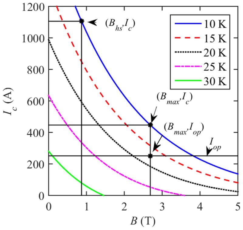
Critical current of the used in the simulations of the 1.5 T magnet, wire as a function of magnetic field strength for various temperatures. Indicated are the operating current, I_c, the critical current at the locations of the maximum magnetic field, B_max, and the critical current at the location of the quench initiation.

In these simulations, the initiation of the quench was started at location on the coil’s surface where the I_op/I_c ratio is low since the NZPV at this location is near its minimum. For both the 1.5 and 3.0 T magnet designs, the maximum temperature would reach more than 400 K if the quench were left to propagate without any protective measures. A passive quench protection system, which does not rely on any external circuitry, triggers, or power supplies, would be ideal but is not possible for HTS magnets [25]. To examine the possibility of successfully protecting the 1.5 and 3.0 T MgB₂ magnets, an active quench protection method is discussed in the next section. The failure mechanisms of the magnet during a quench are mainly due to either the excess strain in the MgB₂ wire or the excess stress in the epoxy. Although the mechanical stress and strain analysis determines whether the magnet would be damaged during a quench, the peak temperature reached during the quench is used as a proxy, and only the quench protections solution where the peak temperature is kept below 200 K as suggested in [25] are considered. Once the quench protection scenarios where the peak temperature is kept below 200 K are found, a complete analysis of the stress and strain within the coil bundles is then performed.

7.2. Active quench protection method

The goal of the active quench protection system is to intentionally quench as much of the magnet as quickly as possible in order to distribute the magnetic energy as evenly as possible. The proposed active quench protection system (figure 16) consists of a set of quench heaters on each coil that are powered by a charged capacitor. The switch to the capacitor is activated by the detection of a small voltage (~100mV) developed across one of the coils. In this work, the voltage developed across a single coil was used for quench detection. For faster quench protection, the use of multiple voltage taps within a coil could be considered.

Figure 16.

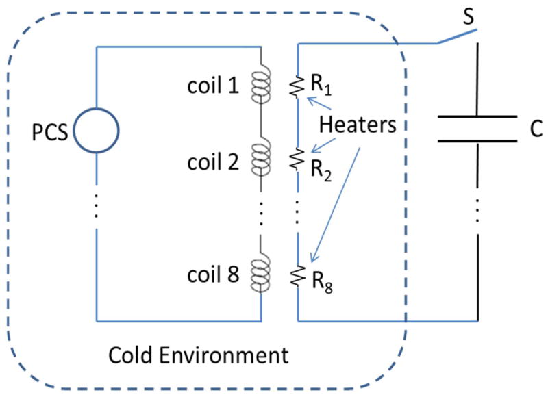
Schematic of an active quench protection system.

When calculating the voltage developed across a coil during a quench, it is important to include the combination of the resistance developed in the wire, the self-inductance of the coil, and the mutual inductance between individual coils. In the quench protection simulations, it is the total voltage that is used to trigger the quench protection. Once the voltage across one of the coils is larger than the threshold voltage of 100 mV, the protection heaters are activated. In this proposed design, the quench protection heaters are placed around the outside of the coils and are simulated by injecting heat into the outer layers of all eight coils.

For the 1.5 T magnet design, the maximum temperature rise can be kept below 200 K by injecting a total of 34.4 kJ into the outer layers of the coils within 0.2 s. This addition of external energy is implemented by storing energy in a capacitor, which is then connected to the quench protection heaters forming an RC circuit with time constant τ = RC. The RC circuit is switched on for only 0.2 s to avoid dumping all of the stored energy in the capacitor into the magnet. In this scenario, only a fraction of the initial stored energy in the capacitor is delivered to the quench heaters due to the exponential decay of the RC circuit. For the combinations of capacitors and heater resistances used in the 1.5 and 3.0 T magnet designs, only 18% of the total stored energy is delivered to the coils. Although a more efficient method for delivering power to the heaters is preferred, implementing the concept of capacitor powered heaters demonstrates that the magnet can be protected from damage during a quench if 34.4 kJ can be delivered to the heaters within 0.2 s.

In this design, the protection heaters are placed on the surfaces of all the coils. In principle, the protection heaters could also be wound within the coils leading to a more uniform distribution of heat. However, this heater design would be more difficult to manufacture, so the protection heaters are only placed on the surfaces of the coils in this paper. A hot spot is initiated by setting a region on the surface of a coil to the resistive state [59]. The quench then develops until it can be detected when the total voltage across a coil exceeds the quench detection threshold voltage, V_th. Upon detection, the quench protection system is activated, and power is delivered to the quench protection heaters. If the quench is detected earlier, the protection mechanism is also initiated earlier, and the peak temperature of the coil will be lowered. The precise choice of threshold voltage will be determined in part by the noise level on the voltage taps. A trade-off exists between a more robust trigger at a higher voltage but lengthier delay to trigger the quench heaters, and a lower voltage threshold more susceptible to false triggers. For these simulations, the quench protection heaters were triggered when the voltage across the quenched coil becomes greater than 100 mV [74]. A simulation of the quench propagation with this quench protection for the 1.5 T magnet gives the maximum temperature in each coil (figure 17) and leads to the conclusion that the peak temperature can be kept below 200 K.

Figure 17.

The maximum temperature in each coil bundle as a function of time for the 1.5 T magnet design. The quench protection is triggered when the voltage on coil 1 reaches 100 mV.

For the 3.0 T magnet design, the maximum temperature is no longer limited to under 200 K, but reaches temperatures significantly above 200 K as seen from figure 18. In order to limit the maximum temperature for the 3 T design to under 200 K, the Monel sheath can be replaced by a Glidcop sheath, which reduces the maximum temperature to under 200 K (figure 19).

Figure 18.

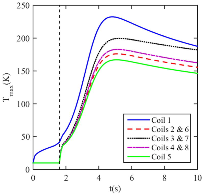
The maximum temperature as a function of time for the 3.0 T magnet design with the Monel sheath. The quench protection is triggered when the voltage on coil #1 reached 100 mV.

Figure 19.

The maximum temperature as a function of time for the 3.0 T magnet design with the Glidcop Sheath. The quench protection is triggered when the voltage on coil #1 reached 100 mV.

7.3. Mechanical stress and strain during a quench

Once the temperature in the coils has been calculated, an ANSYS simulation verifies that the stress and strain in the MgB₂ superconductor and the epoxy insulation are well within the safety factor limit of 0.2% strain. The analysis is focused mainly on the MgB₂ strain development. Along with the strain development, the shear stress in the epoxy also needs to be considered. The constituent elements of the composite wire (copper, Monel and niobium) are numerically homogenized. Instead of considering all 18 superconducting filaments, one equivalent single filament of MgB₂ and epoxy layer is considered in the RVE for quench analysis. In ANSYS simulations, the geometry of the wire was simplified as shown in figure 20. Although simplified, this geometry is beneficial in analyzing the stress and strain scenarios on the MgB₂ filaments and the epoxy. It was assumed that the temperature in the Monel/Cu/Nb/MgB₂ conductor was uniform in the radial and axial directions: all temperature gradients occur in the insulation or along the wire in the azimuthal direction. For input to the ANSYS calculations, the temperature in the epoxy was determined by a linear interpolation of the conductors on either side of the insulation.

Figure 20.

Representative volume element (RVE) as considered for quench stress and strain analysis.

For the CTD-101K epoxy, the MgB₂, and the Monel/Cu/Nb composite of the wire RVE (figure 20), the thermal strains (referenced to a temperature of 10 K) are calculated for use in ANSYS simulations

$${\epsilon }_i(T)\equiv {\int }_{10\mathrm{K}}^T{\alpha }_i(T)\mathrm{d}T,$$ (2)

where ε_i(T) is the accumulated thermal strain at temperature T (referenced to 10 K), and α_i(T) is temperature dependent thermal expansion coefficient in the r, θ, and z directions. The references for the temperature dependent material properties are given in [54]. The accumulated thermal strains are shown in figure 21(a). In these simulations, the materials are isotropic except for the epoxy. The epoxy has two coefficients of thermal expansion: one in the warp or fill direction, which is along the direction of the wire (θ direction), and the other in the through thickness direction, which is perpendicular to the wire (r and z directions). The MgB₂ is assumed to be isotropic, and the Monel/Cu/Nb composite was numerically homogenized [47], where the average stress is computed for the applied unit strain of the composite. Similarly, the modulus of elasticity (figure 21(b)) for the epoxy (CTD-101K), the MgB₂, and the Monel/Cu/Nb composite of the wire RVE are calculated for use in the ANSYS calculations. The Poisson’s ratios are 0.33 for the Monel/Cu/Nb composite, 0.3 for the epoxy, and 0.18 for the MgB₂ [54].

Figure 21.

Thermal strain and elastic modulus used in ANSYS simulations: (a) the accumulated thermal strain is referenced to T = 10 K; (b) elastic modulus.

The strain and stress development in MgB₂ and epoxy respectively is calculated for both the 1.5 and 3.0 T magnet designs. The first principal strain and maximum shear stress results for 1.5 T 100 mV detection are presented in figure 22(a) and (b) respectively. For the 1.5 T magnet, the stress and strains were determined for both 100 and 200 mV quench detection simulations. For 3.0 T coil, both 1542 and 1542G wires are considered. The results are summarized in table 9.

Figure 22.

Strains and stresses calculated in ANSYS during the quench simulation of the 1.5 T magnet. (a) Tensile strain in the MgB₂ superconductor; (b) maximum shear stress in the epoxy insulation.

Table 9.

Maximum stress and strain in 1.5 and 3.0 T magnets during a quench.

System	First principal strains (%) MgB2	Maximum shear stress (MPa) Epoxy	Temp (K)
1.5 T magnet	0.0795	52.5	189
Wire #1027 Vth = 100 mV
1.5 T magnet	0.0894	58.9	216
Wire #1027 Vth = 200 mV
3.0 T magnet	0.1133	90.1	232
Wire #1542 Vth = 100 mV
3.0 T magnet	0.0915	82.9	183
Wire #1542G Vth = 100 mV

From table 9, the strain in the MgB₂ is well below the safety factor design limit of 0.2% even if superimposed on the strain values at the time of winding, cool down, and electromagnetic charging. Thus, the strain development in MgB₂ is well below the criterion. However, the shear stress development in the epoxy is also a concern during a quench. The maximum shear stress development in the epoxy is reported to be 44 MPa in contrast to the shear strength of CTD-101K of 130 MPa at a temperature of 180 K [75]. Overall, the magnet systems would be considered safe in terms of MgB₂ strain and epoxy shear stress, and the simulations show positive promise for successful building of the magnet.

8. Persistent joints

8.1. Criteria

For current MRI designs, the temporal stability of the main magnetic field is essential. Imaging protocols require 30–60 min sessions to complete, and the main magnetic field cannot fluctuate by more than 0.1 ppm hr⁻¹ without degrading the image quality [76, 77]. This temporal stability is needed whether the MRI magnet is driven continuously with an external power supply or has a persistent current in the superconducting magnets. However, while precision low-drift power supplies do exist, they are quite expensive, and persistent mode operation is highly desirable from a commercial point of view. Most MRI systems are designed with segmented coils, which requires the use of wire-to-wire joints. In addition, the possibility of joints reduces somewhat the need for very long wire lengths. In order to maintain the 0.1 ppm hr⁻¹ magnetic field stability requirements, the electrical resistance of the joints connecting the individual coils must be very low—on the order of 10⁻¹¹ Ω or less per joint. These joints allow the background magnet to operate in a persistent current mode without making adjustments to the gradient coil current or the RF send-and-receive frequency during an imaging sequence.

8.2. Present designs

Persistent joints are fully developed and commercialized components in all existing NbTi MRI systems. In order to operate an HTS- or MgB₂-based MRI in persistent mode, such joints must be developed for these conductors as well. Persistent joints are very difficult in Bi-based and YBCO HTS conductors, because along with their high T_c comes a very short coherence length, as well as a relatively complex chemical structure, both of which make true persistent joint development exceedingly difficult. The difficulty in making persistent joints for HTS superconductors are a major road-block in the development of commercially viable MRI with such wire.

In contrast, MgB₂ persistent joints, formed via a wind-and-react (as is done with Nb₃Sn) have already been experimentally demonstrated [78]. For conductors such as Nb₃Sn and MgB₂, both the coil and persistent joint fabrication must either be wind-and-react (W&R) or react-and-wind (R&W), and the persistent joint method must be compatible with either method. Hyper Tech Research Inc. and OSU are actively developing both approaches, and the constraints on their development are different. For W&R, the wires are flexible before reaction, and the joint would be made and then reacted along with the coil set as a whole. For the more desirable R&W method, the already reacted wires would be joined after they were wound into coils, in which the strain limitations of the conductors must be taken into account. In its reacted state, MgB₂ is intermetallic and has a limited strain tolerance after reaction. NIST has measured the axial tensile strain limit at 0.4% for HTR conductor. Also, measurements of permissible room temperature bending strain after reaction HT have been made by OSU [79].

As noted above, Hyper Tech Research Inc. (joint development) and OSU (joint testing) have been pursuing both W&R and R&W style joints. For each joint type, a preliminary screening test was first applied in the form of a direct four point I–V measurement using the test configuration shown in figure 23. Figure 23(a) shows an external view of a joint with a (patented) design for a R&W mode joint, and figure 23(b) shows the critical current which the joint carries as measured by the screening method (direct I–V ) test (<10⁻¹⁰ Ω). The lowest detectable joint resistance using this technique was 10⁻¹⁰ Ω, but this sensitivity is not low enough to conclude the persistent joint is suitable for MRI magnets.

Figure 23.

MgB₂ persistent joint formed between two reacted (HT 3700) wires, (left) picture of the fixture and a persistent joint, (right) critical current of the joint as a function of B.

To measure joint resistances below the ~10⁻¹⁰ Ω sensitivity of the four-point screening technique, a new fixture, shown in figure 24(a), was designed to create a complete loop of the MgB₂ wire containing the persistent joint and a separate concentric driver coil of NbTi wire to energize the MgB₂ wire loop. A hall probe is inserted within both coils to measure the field of the secondary loop (and the primary loop when excited). The loop test fixture, which contains the driver coil, the ~two loops of MgB₂ wire, and the reaction chamber, are all mounted on a frame (figure 23(a)), which is sized to facilitate the use of a test chamber normally used for measuring 50 mm diameter ITER barrels. The resistance in the loop of MgB₂ wire and persistent joint can be determined from the time decay of the magnetic field in the fixture and the inductance of the loop.

Figure 24.

Loop fixture for direct decay measurements of persistent currents, shown with joint attached.

Two protocols have been used to measure the joints with the fixture shown in figure 24. In both cases, the fixture is inserted into a solenoidal magnet, which applies along the z-axis a field, perpendicular to both the primary and secondary coils. In the first protocol, (1) the field is increased either to turn off the joint or suppress its J_c. (2) The current in the primary coil can be excited, and the field dropped back to a low field, e.g, zero field (switching the joint on). (3) When the primary current is then turned off a persistent current is induced in the secondary coil, which generates a magnetic field that is measured by the hall probe. In the second protocol, the background field serves both to switch off the joint and to induce the persistent currents. The primary coil is not used. (1) The field is increased, (2) and then decreased, and the decay is measured. The field of the background magnet is subtracted from the decayed field, and the field from the secondary coil can be observed. The current in the secondary coil can be determined from this decay as well as its inductance. A W&R style type joint (based on HTR strand 3700) was mounted onto the fixture of figure 24, and the results for the persistent current and its decay to zero background field are shown in figure 25.

Figure 25.

(Left) Decay of persistent current in MgB₂ W&R style joint based on expected MRI style MgB₂ conductor strand HTR 3700 at zero applied field (4.2 K), (right) initial persistent current as a function of field at 4.2 K.

There appeared to be an initial faster decay, but settling out to a zero applied field result where τ = 3.7 × 10⁵ s, and R = 4 × 10⁻¹² Ω. Using this same protocol as a function of field, the persistent current as a function of B is shown in figure 23(b). The joint resistance did change somewhat with an increased field of 3 T, with τ = 2.5 × 10⁵ s and R = 3.8 × 10⁻¹¹ Ω. These resistance values need to be reduced even further, and the same results for joints must be developed with already reacted wires (relevant to a R&W approach).

8.3. Future designs

The goal of fabricating joints relevant for MRI/NMR magnets are continuing to be developed. The process follows a path based on joining reacted multi-filament MgB₂ wires with Mg + 2B powders in situ (figure 23), which enables the independent winding of large coil bundles and subsequent assembly into MRI background magnets. Presently, multiple persistent joints are being manufactured and measured for resistance until their viability and repeatability are assured. Joints have been tested with both a side-by-side connection and an end-to-end connection, both of which are required make the series joint connections between coils.

In the assembly of the magnet, the persistent joints connecting the coil bundles are formed in situ after the individual coil segments have been mounted to their respective positions on the support structure. The wires extending from the coil segments have sufficient length to ensure that the persistent joints can be placed at electrically insulated and thermally sinked locations on the thermal buses. A small portable retort can enclose the persistent joint chamber and heat at each joint in the final assembly of all magnet segments with an induction heater. The retort and reaction chamber must be heated to 650 °C for up to 1 h while continuously purging the area with argon to avoid oxidation. Conceptual designs have been completed but carrying the development forward awaits validation of the laboratory model.

9. Persistent switch

9.1. Persistent switch design

Even though the temporal stability of 0.1 ppm hr⁻¹ required for MRI main magnets can be achieved with a highly regulated (and hence expensive) external power supply, the same stability can be maintained by operating the magnet in persistent current mode, in which the magnet is wired with one continuous loop of superconducting wire. The zero resistance of the wire loop allows current to flow with virtually no resistive loss, and therefore, stable magnetic fields are maintained over long periods of time. The persistent current mode can be implemented only with the use of a persistent switch (PCS). (figure 26) which is included within the loop of superconducting wire making up the magnet.

Figure 26.

Circuit diagram of a persistent current switch (PCS) used to charge a superconducting magnet. (a) The PCS circuit while charging the magnet. The heater keeps the persistent switch in a resistive state, thus the majority of current flows through the magnet. (b) The PCS circuit when heater is removed. The switch becomes a short circuit, allowing all of the current to flow through the superconducting loop, thus achieving persistent mode.

While charging the magnet, the persistent switch is heated to slightly above the superconducting material’s critical temperature and becomes highly resistive compared to the magnet’s inductive impedance (figure 26(a)). Here, only a small amount of current will flow through the switch. Once the magnet is at the desired magnetic field, the persistent switch is cooled back down to below the critical temperature, and the power supply is disconnected (figure 26(b)).

Many considerations and tradeoffs occur in the design of a PCS. While charging the magnet, the switch must be resistive enough (i.e. the switch is in an ‘open’ state) to prevent a significant amount of current flowing through the switch. The switch is ‘opened’ by heating a section of wire so that it is no longer superconducting, and the resistance of the switch is determined by the material composition, cross sectional area, and total length of the switch’s wire and the switch’s temperature. Furthermore, once the magnet has reached the desired magnetic field, the switch must be able to transition back to a superconducting state in a reasonably short time. This process is achieved by heating the switch slightly above the critical temperature of MgB₂ during magnet charging, and requires that the heater provides just enough power to maintain the switch at a temperature slightly above the critical temperature.

The material composition of the wire is an important factor in the design of the persistent switch and the heater. During the magnet ramp-up, most of the current should flow through the magnet, with only a small fraction (e.g. 0.1% of operating current) diverted through the persistent switch. This percentage is chosen as it allows for a small amount of current through the switch while also allowing for the wire to have a reasonable resistance. Essential design input parameters include the magnet operating current, magnet inductance, and charging time.

While charging the magnet, the voltage across the persistent switch is mainly due to the magnet’s inductive voltage V = L × dI/dt, where L is the magnet’s inductance and dI/dt is the slew rate of the current. The resistance R is obtained from Ohm’s law V = IR. Ultimately, an estimation for the length of the MgB₂ wire is required to obtain a resistance R at a given operating temperature. Since the wire is composed of various proportions of MgB₂, Nb, Cu and Monel, the resistivity of the wire can be estimated using the equation of mixtures if the resistivities of the constituent materials at low temperature are known:

$${\rho }_{\text{wire}}={(f_{\text{Cu}}/{\rho }_{\text{Cu}}+f_{\text{Nb}}/{\rho }_{\text{Nb}}+f_{{\text{MgB}}_2}/{\rho }_{{\text{MgB}}_2}+f_{\text{Monel}}/{\rho }_{\text{Monel}})}^{-1}.$$ (3)

The optimal length of the wire in the switch is a tradeoff between minimizing the amount of wire and using low power to avoid overloading the cryocooler. An estimate for the required length at various temperatures could then be obtained and fitted to a power law relation.

The design of the persistent switch usually starts from the specifications of the magnet and requirements on the MRI system. For instance the operating current, I_op, and inductance, L, of the magnet are given and the ramp up time, t_r, should be reasonable. To minimize the amount of resistive power generated in the PCS, the current flowing through the PCS is limited to a small fraction (~0.1%) of the total current in the magnet. The wire type for the PCS can be different than the wire used in the magnet bundles. Within the manufacturing limits, the wire resistance is kept as large as possible by reducing the inductance L, shunt current fraction F, parameters, and associated expressions for the switch are tabulated in table 10.

Table 10.

Design parameters for persistent switch in 1.5 and 3.0 T MRI systems.

Parameter	1.5 T system	3.0 T system
Magnet inductance L	72.2 H	276.1 H	From magnet design
Operating current Iop	251.07 A	252.5 A	From magnet design
Ramp-up time tr	120 min	120 min	From MRI system specification
Shunt current fraction F	0.1%	0.1%	Small to keep heating low
Wire component fraction f	Monel: 38%	Monel: 38%	Based on available wire
	Cu–Ni: 26%	Cu–Ni: 26%	Has a minimum fraction of Cu to increase resistivity
	Nb: 20%	Nb: 20%
	Cu: 2%	Cu: 2%
	MgB2: 14%	MgB2: 14%
Wire diameter d	1 mm	1 mm	Based on available wire
Magnet back EMF ξ	2.52 V	9.68 V	Magnet back EMF ξ = L Iop/tr
Switch resistance R	10.0 Ω	38.3 Ω	R = ξ/(F Iop)
Wire resistivity (@ 60K)	34.4 nΩ m	34.4 nΩ m	(Σ( fi/ρi))−1
Wire cross-sectional area A	0.79 mm2	0.79 mm2	π (d/2)2
Wire length l = l(T)	229 m	876 m	AR/ρ

The basic switch’s design wraps the total length of the MgB₂ wire around a copper bobbin that is in thermal contact with the coolant system of the magnet. A heating element, preferably a resistive wire, is then co-wound with the wire to heat it above the critical temperature during ramp-up. Copper was chosen as the bobbin material due to its high thermal conductivity, which allows it to operate very effectively as well as a cold sink. The cold sink must efficiently draw heat away from the device once the current to the heater is turned off.

Also, the MgB₂ wire needs to wrap around the bobbin in a non-inductive manner to prevent the generation of any magnetic field inside the PCS, which would negatively affect the flow of current through the switch and the static field of the main magnet. This non-inductive wrapping is achieved by using the MgB₂ wire in a bifilar configuration depicted in figure 27. The MgB₂ wire is co-wound with the heater wire to ensure uniform heating when the PCS is in resistive mode. A bifilar build is achieved by starting at the mid-point of the total superconductor wire-plus-heater length and doubling it back onto itself forming the bifilar bundles consisting of two sets side by side of one MgB₂ wire and two heater wires (figure 28).

Figure 27.

Bifilar wire built for a MRI persistent switch using MgB₂ superconductor. Note that two heater wires are used for redundancy. By twisting the three-wire bundle 180° at the mid-point fold, a close-packed build is achieved.

Figure 28.

Persistent switch with bifilar MgB₂ wire and heater winding.

9.2. Analytical results

Using the design parameters above and applying the theory of mixtures to account for temperature effects, the shunt resistances needed are R = 10.03 Ω and 38.35 Ω for the 1.5 T and 3.0 T systems, respectively. Applying the method outlined above, the temperature-dependent resistivity and corresponding length of the composite wire needed to attain the shunt resistance for each system is plotted in figure 29. The copper bobbin, on which the wire is wound, must be able to fit within the spatial limitations inside the cryostat. A reasonable option and resulting winding arrangement for each system is listed in table 11. The superconductor is operated below both the transition temperature of MgB₂ of 39K and the critical current value at the desired magnetic field and temperature so that no power loss occurs. During the charging of the magnet, the superconductor is operated above the critical temperature to provide resistance. For illustrative purposes, a switch temperature of 60 K was selected for both the 1.5 T and 3.0 T systems, giving nominal wire lengths of 229m and 876 m, respectively.

Figure 29.

Plot of wire length versus temperature for the 1.5 T system using data in table 10.

Table 11.

Copper bobbin parameters and winding arrangement for the selected wire length for a switch operating at 60 K.

Magnet system	Radius (cm)	Height (cm)	Number of turns	Number of layers	Total radius (cm)
1.5 T	6	10.00	41	7	14.4
3.0 T	6	10.00	41	22	19.5

The temperature of the persistent switch during both the ramp-up and cool-down was modeled using the TEMPO module in Vector Fields (Cobham Technical Services). For the ramp-up process, the persistent switch’s heating element is set to 10 W, and the switch’s temperature as a function of time is calculated to determine the how long the switch takes to reach 60 K (figure 30(a)). To reach 60 K, it took 37 min for the 1.5 T persistent switch and 108 min for the 3.0 T persistent switch. For the cool-down process, the initial temperature distribution was determined from the steady state temperature distribution (60 K inside the switch using 5 W in the heating element). The transient simulation was run using the mentioned above temperature distribution with no internally generated heat inside the switch. To cool down to 10 K, it took 108 min for the 1.5 T persistent switch and 220 min for the 3.0 T persistent as shown in figure 30(b). The results of this study are summarized in table 12.

Figure 30.

Temperature of the persistent switch for the 1.5 and 3.0 T magnet designs during (a) heating of switch, and (b) cool-down of switch. The switch parameters are given in table 11.

Table 12.

Ramp-up and cool-down time obtained by numerical simulations for the switch operating at 60 K in table 11.

Magnet system	Static temperature (K)	Ramp-up heater (W)	Ramp-up time to 60 K (min)	Cool-down time to 10 K (min)
1.5 T	59.7	10	37	70
3.0 T	60.3	10	108	220

10. Commercialization

The interest in MgB₂ superconductor wire for conduction cooled MRI background magnets is driven by the current market for LHe. Over the last ten years the cost of LHe has increased over 300% and is expected to increase continually over the coming years, and the worldwide demand for helium over the last five years nearly matches the potential level of supply, which also drives up the cost. In 2015, the retail cost of LHe ranged from $10–50 per liter based on quantity and location around the world, and is still increasing each year.

Over the last seven years, local shortages have resulted when certain LHe facilities had closed temporarily for maintenance. These issues of the rising cost and availability of helium are inevitable since it is extracted from natural gas, and only certain natural gas fields have high enough helium percentage to make its extraction worthwhile. Presently, about 25% of the helium used each year is for MRI systems either for filling new MRI’s or refilling and topping off old machines. While all current 1.5 and 3.0 T MRI systems use a re-condensing system for helium, helium is needed both for the initial filling of the magnet and for refilling or topping off the magnet if the magnet quenches at the hospital.

Already MgB₂ conduction cooled MRI magnets are making their way into the market place for specialty applications. Two such applications include: an open MRI for orthopedic examinations where a patient can be imaged while putting weight on their joints, and an MRI coupled with a radiation therapy device for treating cancer patients. These two applications cannot be typically done in a solenoidal full body MRI.

The helium cost is saved in two other ways. First, during the initial fill at the manufacturer LHe is consumed during the initial cooling and training of the NbTi coils. Second, if the magnet quenches at a hospital, most of the LHe is lost through the venting system, so the magnet must be refilled with LHe. Conduction cooled full body MRI systems will bring additional benefits to the market place. Some areas of the world do not have the logistical network to supply the LHe needed for topping off or refilling an MRI. Conduction cooled MgB₂ magnet systems use a cryocooler (compressor and cold head) with a small quantity of helium (~1 l) in a closed loop. This helium can be supplied under pressure in small gaseous helium cylinders and shipped to remote locations, where it is held at the sight until it is needed for maintenance. Reliability is also an issue. Because of the small temperature margin of 1 K for NbTi magnets, the magnet might quench, which would shut down the hospital’s imaging capability. By contrast, the extra temperature margin for MgB₂ magnets will greatly reduce the potential for non-emergency magnet quenches. Safety is another concern. Inside the present MRIs, the helium is contained in a vessel with the main magnet coils at near atmospheric pressure. However, during a quench, the sudden pressure rise places the vessel under much pressure until the generated gaseous helium vents. Because of this increased pressure, the vessel is required to be classified as an ASME section 8 pressure vessel. With a conduction cooled magnet, this required vessel classification is not necessary, which thereby eliminates a rupture potential and the need for a pressure vessel. In addition to cost savings from eliminating the pressure vessel, the elimination of the rupture disc and ducting to the outside of the hospital to release the helium to the outside during a quench would also reduce costs. Most 1.5 and 3.0 T MRI magnets are filled with LHe at the factory for testing and shipped this way. NbTi magnets require training (multiple quenches) before shipping to the assembler. While the helium in the plant is now captured and re-liquefied, about 25% is lost, and for the helium liquefier and an on-going cost for its maintenance gives an initial expense. A continuous loss of helium occurs when transporting the MRI magnet without the continuous operation of the re-liquefying cryocooler as there is at the factory or user site, This loss places a tight time constraint on shipping the LHe in order to minimize its loss. As a consequence, many of these filled LHe MRI’s are expensively shipped to their location by air. Once at the hospital, the magnet is topped off with additional LHe to compensate for the loss. Purchasing LHe in the field is more expensive than in the magnet factory. With conduction cooling, no helium is needed in the factory for testing, and the magnet can be warmed up for shipping as dictated by other time constraints. The shipping has fewer logistics requirements and is cheaper since the magnet can be transported either by land and/or sea. In addition, a large quantity of helium is not needed for the magnet cool down at the hospital.

10.1. Impediments to the adoption of conduction cooled MgB₂ magnets for 1.5 and 3.0 T MRI?

While considerable progress has been made with the development of MgB₂ magnets, more progress is needed to implement the full conversion and replacement of NbTi wire for MRI full body background magnets at 1.5 and 3.0 T. The magnet technology can be developed and demonstrated today but must reach a price point to replace NbTi helium bath cooled magnets. While the price performance of MgB₂ wires for MRI has come down significantly, it still needs to be reduced so the overall cost of MRI systems to hospitals is not increased. More required improvements have been discussed in this paper. It is amazing how much progress has been made with MgB₂ superconductor wires over the last few years with very limited funding compared to the funding that has been spent on the development of higher temperature superconductors such as BSCCO and YBCO. In spite of the limited funding, work worldwide is continuing to lead to designing, building, and testing MgB₂ conduction cooled 1.5 T full body MRI magnet systems. In the last couple of years, the discovery and demonstration of dramatically improved MgB₂ wires (2nd generation) in short samples may lead, when demonstrated in long lengths, lead to the price performance for the wire to make it comparable to the price/performance of NbTi wires. In addition, Progress reported in this paper has shown that persistent joints with reacted MgB₂ wires are possible. Further work on the improvement of persistent joints and persistent switches will also continue.

11. Conclusions

Following the discovery of the superconducting properties of MgB₂ in 2001, tremendous progress has been made in the development of MgB₂ superconducting wire. It is now possible to manufacture MgB₂ superconducting wire in lengths greater than 10 km with a cross sectional area less than 1 cm², that can support several hundred amperes of current. Using this type of wire, prototype magnet coils with dimensions and currents similar to MRI magnet coils have been constructed and experimentally tested when cooled with LHe to temperatures of 4.2 K. MgB₂ superconducting wire has also been used commercially, for example, in Paramed’s OpenSky 0.5 T MRI magnet. In addition, persistent joints, formed via a wind-and-react, have been experimentally demonstrated with MgB₂ wire, and progress has been made in forming MgB₂ persistent joints using react-and-wind, multi-filamentary wire.

Since the majority of today’s clinical MRI systems use 1.5 and 3 T magnets, the feasibility of MRI magnets at these field strengths using MgB₂ superconducting wire should be explored. Additionally, there is a need to move away from LHe cooled magnets to reduce the risk of LHe supply disruptions and the rising demand for this limited natural resource. With a critical temperature of 39 K, MgB₂ superconducting wire can facilitate conduction cooled 1.5 T or 3.0 T magnets that eliminate the need for LHe.

To investigate the viability of such MRI magnets, conceptual designs for 1.5 and 3.0 T conduction cooled MgB₂ MRI magnets were completed. The transport properties of available MgB₂ superconducting wire are presented and assessed for their use in magnet designs. The capability already exists to manufacture wire with the size, geometry, and composition that serves as the basis for the magnet design. Potential improvements in the performance of MgB₂ wire (i.e 2nd generation wire) would be beneficial and allow for more design flexibility. However, the conceptual designs in this paper use the properties of available wire and do not rely on future improvements in wire performance.

Using optimization techniques, a magnet coil geometry was found for each of the 1.5 and 3.0 T MRI magnets. Both designs use eight coil bundles to generate a magnetic field with an inhomogeneity of less than 10 ppm over the 45 cm DSV and are self-shielded to limit the magnetic field to less than 5 Gauss in areas outside of the typical MRI installation site. The size of the MgB₂ wire (including the insulation and epoxy between wires) was chosen to be a 1.19mm × 1.81mm rectangle, which is considered realistic in terms of manufacturability. For the 1.5 T magnet, a wire with 10%MgB₂ and 27% Cu was assumed, and for the 3.0 T magnet, a wire with 15% MgB₂ and 42% Cu was assumed.

A conduction cooling system was designed around the coil geometries and uses copper straps and cooling rings to transfer heat from the coil windings to a two stage cryocooler. A detailed 3D model of the cryocooler, copper conduction path, superinsulation, and vacuum vessel was used to calculate the heat load due to thermal radiation. It was concluded that the heat load from the thermal radiation is expected to be 20W at the first stage of the cryocooler and 0.4W at the second stage. The temperature gradient within the coil is expected to be less than 2 K. An estimation of the total heat load (including heat loss from mechanical supports, charging leads, and instrumentation) is 58W at the first stage and 0.6W at the second stage. Further modeling is needed to verify the accuracy of these estimations, but the initial results suggest that conduction cooling of the MgB₂ magnet to a temperature of 10 K is a viable.

Detailed ANSYS simulations of the mechanical stress and strain within the coil bundle during manufacturing, cool down, and energizing were completed. In particular, the focus was on the strain developed within the MgB₂ and the sheer stress within the epoxy, and it is concluded that these magnet designs could operate under normal conditions without mechanical failure.

A major concern for HTS magnets is the protection of the magnet during a quench. It is concluded that an active quench protection is necessary to protect the magnet, and a conceptual design of a quench protection system is proposed. Numerical simulations of the NZPV and MQE for the 1.5 and 3.0 T magnet designs was completed and support the conclusion that the quench propagation in the magnets is too slow to consider passive quench protection.

A finite difference technique was used to calculate the temperature profile developed during a quench. The model includes the thermal propagation within the wire and epoxy, the critical current of the MgB₂ wire, the self and mutual inductances of the coils, and the current decay of in the magnet. Without intervention, it is found that the temperature within the magnet during a quench would exceed 400 K. Calculations of the quench propagation using the proposed active protection system demonstrate that the maximum temperature could be limited to below 200 K. To verify whether the magnet could survive a quench, the temperature profile from the quench simulations is used as an input for an ANSYS calculation of the stress and strain developed during a quench. From these situations, the stress and strain do not exceed the failure limits for either the MgB₂ wire or the epoxy.

The progress in the development of MgB₂ persistent joints is reported, and the fabrication of persistent joints of multi-filamentary, react and wind, MgB₂ superconducting wire at the quality level needed for persistent current operations of MRI systems shows real promise. A design of a persistent switch is given to demonstrate the feasibility of building a switch, fitting it into the vacuum vessel, and turning the switch on and off in a reasonable amount of time.

The possibility of a conduction cooled MgB₂ 1.5 and 3.0 T MRI magnets has been demonstrated at a conceptual level. While a considerable amount of progress has been made with the development of MgB₂ magnets, converting a conceptual design into a complete design requires significant engineering effort. Among these include the design of a mechanical support system to handle the large magnetic forces on the coil bundle while at the same time minimizing the heat leak through the support structures. With a more complete mechanical support system developed, the heat loads and temperature profiles can be calculated with more accuracy. Among the challenges in this regard is careful consideration of the bolted connections between the copper components in the conduction cooling system to ensure a good thermal contact. While an active quench protection has been proposed, it relies on a capacitors with a total stored energy of over 150 kJ. While technically possible, this active protection system may not a palatable option due to safety concerns in a clinical MRI setting.

In summary, there has been tremendous progress in the development of MgB₂ superconductor wire technology, MgB₂ test coils and magnet design, and MgB₂ superconducting wire has been used in commercial products. Building on this success, we have developed a conceptual design for 1.5 and 3.0 T conduction cooled MRI magnet using available MgB₂ superconducting wire. Further engineering and is needed to translate these conceptual designs into complete, ready-to-build, designs. As replacements for 1.5 T and 3.0 NbTi MRI systems, these magnets have the potential to reduce the MRI industry reliance on LHe. Adoption of these magnets commercially will depend on improvements in MgB₂ wire performance, the supply and demand of LHe, and manufacturing costs of superconducting MgB₂ magnets. With over 35 000 MRI systems worldwide, the development of MgB₂ superconducting, conduction-cooled, 1.5 and 3.0 T MRI systems is a worthwhile goal.

Figure 4.

The critical current I_c in the wire at temperature T = 10 K as function magnet field of strength B for: (a) wire type #1027 used in the 1.5 T magnet design, and (b) wire types #1542 and #1524G used in the 3.0 T magnet designs [36]. These plots are for the wire at a temperature of 10 K. The maximum field on wire and the corresponding critical current are indicated in each plot.

References

- 1.Lvovsky Y, Stautner EW, Zhang T. Novel technologies and configurations of superconducting magnets for MRI. Supercond Sci Technol. 2013;26:93001. [Google Scholar]
- 2.Lvovsky Y, Jarvis P. Superconducting systems for MRI-present solutions and new trends. IEEE Trans Appl Supercond. 2005;15:1317–25. [Google Scholar]
- 3.Spencer C, Sanger PA, Young M. The temperature and magnetic field dependence of superconducting critical current densities of multifilamentary Nb3Sn and NbTi composite wires. IEEE Trans Magn. 1979;15:76–9. [Google Scholar]
- 4.Nuttall W, Clarke R, Glowacki B. In: The Future of Helium as a Natural Resource. Nuttall W, et al., editors. Abingdon, UK: Routledge; 2012. [Google Scholar]
- 5.Cai Z, Clarke RH, Glowacki BA, Nuttall WJ, Ward N. Ongoing ascent to the helium production plateau—insights from system dynamics. Resour Policy. 2010;35:77–89. [Google Scholar]
- 6.Espy MA, Magnelind PE, Matlashov AN, Newman SG, Sandin HJ, Schultz LJ, Sedillo R, Urbaitis AV, Volegov PL. Progress toward a deployable SQUID-based ultra-low field MRI system for anatomical imaging. IEEE Trans Appl Supercond. 2015;25:1–5. [Google Scholar]
- 7.Morita H, Okada M, Tanaka K, Sato J, Kitaguchi H, Kumakura H, Togano K, Itoh K, Wada H. 10 T conduction cooled Bi-2212/Ag HTS solenoid magnet system. IEEE Trans Appl Supercond. 2001;11:2523–6. [Google Scholar]
- 8.Baig T, Yao Z, Doll D, Tomsic M, Martens M. Conduction cooled magnet design for 1.5 T, 3.0 T and 7.0 T MRI systems. Supercond Sci Technol. 2014;27:125012. [Google Scholar]
- 9.Miyazaki H, Iwai S, Tosaka T, Tasaki K, Hanai S, Urata M, Ioka S, Ishii Y. Development of a 5.1 T conduction-cooled YBCO coil composed of a stack of 12 single pancakes. Physica C. 2013;484:287–91. [Google Scholar]
- 10.Young MA, Demko JA, Gouge MJ, Pace MO, Lue JW, Grabovickic R. Measurements of the performance of BSCCO HTS tape under magnetic fields with a cryocooled test rig. IEEE Trans Appl Supercond. 2003;13:2964–7. [Google Scholar]
- 11.Wang Q, Song S, Lei Y, Dai Y, Zhang B, Wang C, Lee S, Kim K. Design and fabrication of a conduction-cooled high temperature superconducting magnet for 10 kJ superconducting magnetic energy storage system. IEEE Trans Appl Supercond. 2006;16:570–3. [Google Scholar]
- 12.Bud’ko SL, Lapertot G, Petrovic C, Cunningham CE, Anderson N, Canfield PC. Boron isotope effect in superconducting MgB2. Phys Rev Lett. 2001;86:1877–80. doi: 10.1103/PhysRevLett.86.1877. [DOI] [PubMed] [Google Scholar]
- 13.Buzea C, Yamashita T. Review of the superconducting properties of MgB2. Supercond Sci Technol. 2001;14:R115. [Google Scholar]
- 14.Nagamatsu J, Nakagawa N, Muranaka T, Zenitani Y, Akimitsu J. Superconductivity at 39 K in magnesium diboride. Nature. 2001;410:63–4. doi: 10.1038/35065039. [DOI] [PubMed] [Google Scholar]
- 15.Ling J, Voccio J, Kim Y, Hahn S, Bascunan J, Park DK, Iwasa Y. Monofilament wire for a whole-body MRI magnet: superconducting joints and test coils. IEEE Trans Appl Supercond. 2013;23:6200304. doi: 10.1109/tasc.2012.2234183. [DOI] [PMC free article] [PubMed] [Google Scholar]
- 16.Tomsic M, Rindfleisch M, Yue J, McFadden K, Phillips J, Sumption MD, Bhatia M, Bohnenstiehl S, Collings EW. Overview of MgB2 superconductor applications. Int J Appl Ceram Technol. 2007;4:250–9. [Google Scholar]
- 17.Mine S, Xu M, Buresh S, Stautner W, Immer C, Laskaris ET, Amm K, Grasso G. Second test coil for the development of a compact 3 T magnet IEEE Trans. Appl Supercond. 2013;23:4601404. doi: 10.1109/TASC.2014.2364396. [DOI] [PMC free article] [PubMed] [Google Scholar]
- 18.Yao W, Bascunan J, Kim W-S, Hahn S, Lee H, Iwasa Y. A solid nitrogen cooled demonstration: coil for MRI applications. IEEE Trans Appl Supercond. 2008;18:912–5. doi: 10.1109/tasc.2008.920836. [DOI] [PMC free article] [PubMed] [Google Scholar]
- 19.Bascunan J, Lee H, Bobrov ES, Hahn S, Iwasa Y, Tomsic M, Rindfleisch M. A 0.6 T/650 mm RT bore solid nitrogen cooled demonstration coil for MRI—a status report. IEEE Trans Appl Supercond. 2006;16:1427–30. doi: 10.1109/TASC.2005.864456. [DOI] [PMC free article] [PubMed] [Google Scholar]
- 20.Yao W, Bascuan J, Hahn S, Iwasa Y. MgB2 Coils for MRI Applications. IEEE Trans Appl Supercond. 2010;20:756–9. doi: 10.1109/TASC.2010.2044035. [DOI] [PMC free article] [PubMed] [Google Scholar]
- 21.Park DK, Hahn S, Bascunan J, Iwasa Y. Active protection of an MgB2 test coil. IEEE Trans Appl Supercond. 2011;21:2402–5. doi: 10.1109/TASC.2010.2095812. [DOI] [PMC free article] [PubMed] [Google Scholar]
- 22.Park DK, Ling J, Rindfleisch M, Voccio J, Hahn S, Bascunan J, Tomsic M, Iwasa Y. MgB2 for MRI magnets: test coils and superconducting joints results. IEEE Trans Appl Supercond. 2012;22:4400305. doi: 10.1109/TASC.2012.2185472. [DOI] [PMC free article] [PubMed] [Google Scholar]
- 23.Cosmus TC, Parizh M. Advances in whole-body MRI magnets. IEEE Trans Appl Supercond. 2011;21:2104–9. [Google Scholar]
- 24.Lvovsky Y, Stautner EW, Zhang T. Novel technologies and configurations of superconducting magnets for MRI. Supercond Sci Technol. 2013;26:93001. [Google Scholar]
- 25.Iwasa Y. Case Studies In Superconducting Magnets: Design And Operational Issues. Berlin: Springer; 2009. [Google Scholar]
- 26.Dhallé M, van Weeren H, Wessel S, Ouden den A, Kate ten HHJ, Hušek I, Kováč P, Schlachter S, Goldacker W. Scaling the reversible strain response of MgB2 conductors. Supercond Sci Technol. 2005;18:S253. [Google Scholar]
- 27.Li G, Zwayer JB, Kovacs CJ, Susner M, Sumption MD, Rindfleisch M, Thong CJ, Tomsic M, Collings EW. Transport critical current densities and n-values of multifilamentary wires at various temperatures and magnetic fields. IEEE Trans Appl Supercond. 2014;24:1–5. [Google Scholar]
- 28.Li GZ, Sumption MD, Susner MA, Yang Y, Reddy KM, Rindfleisch MA, Tomsic MJ, Thong CJ, Collings EW. The critical current density of advanced internal-Mg-diffusion-processed MgB2 wires. Supercond Sci Technol. 2012;25:115023. [Google Scholar]
- 29.Bessette D, Mitchell N. Review of the results of the ITER toroidal field conductor R & D and qualification. IEEE Trans Appl Supercond. 2008;18:1109–13. [Google Scholar]
- 30.Xu X, Sumption M, Peng X, Collings EW. Refinement of Nb3Sn grain size by the generation of ZrO2 precipitates in Nb3Sn wires. Appl Phys Lett. 2014;104:82602. [Google Scholar]
- 31.Xu X, Sumption MD, Peng X. Internally oxidized Nb3Sn strands with fine grain size and high critical current density. Adv Mater. 2015;27:1346–50. doi: 10.1002/adma.201404335. [DOI] [PubMed] [Google Scholar]
- 32.Cheng Y-CN, Eagan TP, Brown RW, Shvartsman SM, Thompson MR. Design of actively shielded main magnets: an improved functional method. Magn Reson Mater Phys Biol Med. 2003;16:57–67. doi: 10.1007/s10334-003-0012-x. [DOI] [PubMed] [Google Scholar]
- 33.Lee YS, Chung WH. Method of manufacturing MgB2 superconducting wire. 20090011942 A1 US Patent. 2009
- 34.CTD Materials. www.ctd-materials.com/wordpress/wp-content/uploads/2014/05/CTD-101G-DS-2006.pdf.
- 35.Malagoli A, Tropeano M, Cubeda V, Bernini C, Braccini V, Fanciulli C, Romano G, Putti M, Vignolo M, Ferdeghini C. Study of the superconducting and thermal properties of ex situ glidcop-sheathed practical conductors. IEEE Trans Appl Supercond. 2009;19:3670–4. [Google Scholar]
- 36.Yang Y, Susner M, Sumption MD, Rindfleisch M, Tomsic M, Collings EW. Influence of strand design, boron type, and carbon doping method on the transport properties of powder-in-tube MgB2-XCX strands. IEEE Trans Appl Supercond. 2011;22:6200110. [Google Scholar]
- 37.Cheng Y-C, Brown RW, Thompson MR, Eagan TP, Shvartsman SM. A comparison of two design methods for MRI magnets. IEEE Trans Appl Supercond. 2004;14:2008–14. [Google Scholar]
- 38.Caldwell J. The stress in the windings of a coil carrying an electric current. J Phys D: Appl Phys. 1980;13:1379. [Google Scholar]
- 39.Poole C, Baig T, Deissler RJ, Doll D, Tomsic M, Martens M. Numerical study on the quench propagation in a 1.5 T MgB2 MRI magnet design with varied wire compositions. Supercond Sci Technol. 2016;29:44003. [Google Scholar]
- 40.Rybakov A, Bagdinov A, Demikhov E, Kostrov E, Lysenko V, Piskunov N, Tysyachnykh Y. 1.5 T cryogen free superconducting magnet for dedicated MRI. IEEE Trans Appl Supercond. 2016;26:1–3. [Google Scholar]
- 41.Inoue T, Yokoyama S. Conduction cooling superconducting magnet device. 8269587 US Patent. 2012
- 42.Parkinson BJ, Slade R, Mallett MJD, Chamritski V. Development of a cryogen free 1.5 T YBCO HTS magnet for MRI. IEEE Trans Appl Supercond. 2013;23:4400405. [Google Scholar]
- 43.Terao Y, Ozaki O, Ichihara C, Kawashima S, Hase T, Kitaguchi H, Kobayashi S, Sato K, Nakajima I, Oonishi N. Newly designed 3 T MRI magnet wound with Bi-2223 tape conductors. IEEE Trans Appl Supercond. 2013;23:4400904. [Google Scholar]
- 44.Kar S, Soni V, Konduru P, Sharma RG, Kanjilal D, Datta TS. Quench characteristics of 6 T conduction-cooled NbTi magnet system. IOP Conf Ser Mater Sci Eng. 2015;101:012077. [Google Scholar]
- 45.Rao KR. Companion guide to the ASME boiler & pressure vessel code: Criteria and Commentary on Select Aspects of the ASME Boiler & Pressure Vessel and Piping Codes. Vol. 2. New York: ASME; 2002. section 7. [Google Scholar]
- 46.Green MA. Lessons learned concerning the use of 4 K coolers to cool LTS magnets. Proc. ICC-18; Syracuse, NY, USA. 9–12 June 2014; 2014. pp. 567–76. [Google Scholar]
- 47.Barbero EJ. Finite Element Analysis of Composite Materials Using ANSYS®. 2. Boca Raton, FL: CRC Press; 2013. [Google Scholar]
- 48.Swan CC, Kosaka I. Voigt–Reuss topology optimization for structures with linear elastic material behaviours. Int J Numer Methods Eng. 1997;40:3033–57. [Google Scholar]
- 49.Li L, Ni Z, Cheng J, Wang H, Wang Q, Zhao B. Effect of pretension, support condition, and cool down on mechanical disturbance of superconducting coils. IEEE Trans Appl Supercond. 2012;22:3800104. [Google Scholar]
- 50.Arp V. Stresses in superconducting solenoids. J Appl Phys. 1977;48:2026–36. [Google Scholar]
- 51.Caldwell J. Electromagnetic forces in high field magnet coils. Appl Math Model. 1982;6:157–60. [Google Scholar]
- 52.Boso DP. A simple and effective approach for thermo-mechanical modelling of composite superconducting wires. Supercond Sci Technol. 2013;26:45006. [Google Scholar]
- 53.Boso DP, Lefik M, Schrefler BA. Homogenisation methods for the thermo-mechanical analysis of Nb3Sn strand. Cryogenics. 2006;46:569–80. [Google Scholar]
- 54.Amin AA, Baig T, Deissler RJ, Yao Z, Tomsic M, Doll D, Akkus O, Martens M. A multiscale and multiphysics model of strain development in a 1.5 T MRI magnet designed with 36 filament composite MgB2 superconducting wire. Supercond Sci Technol. 2016;29:55008. [Google Scholar]
- 55.Kováč P, Kopera L, Melišek T, Rindfleisch M, Haessler W, Hušek I. Behaviour of filamentary MgB2 wires subjected to tensile stress at 4.2 K. Supercond Sci Technol. 2013;26:105028. [Google Scholar]
- 56.Orifici AC, Herszberg I, Thomson RS. Review of methodologies for composite material modelling incorporating failure. Compos Struct. 2008;86:194–210. [Google Scholar]
- 57.Fu M, Pan Z, Jiao Z, Kumakura H, Togano K, Ding L, Wang F, Zhang Y, Chen Z, Chen J. Quench characteristics and normal zone propagation of an MgB2 superconducting coil. Supercond Sci Technol. 2003;17:160. [Google Scholar]
- 58.Ghosh AK, Prodell A, Sampson WB, Scanlan RM, Leroy D, Oberli LR. Minimum quench energy measurements on prototype LHC inner cables in normal helium at 4.4 K and in superfluid He at 1.9 K. IEEE Trans Appl Supercond. 1999;9:257–60. [Google Scholar]
- 59.Deissler RJ, Martens M, Baig T, Poole C, Amin AA, Doll D, Tomsic M. Numerical simulation of quench protection for a 1.5 T persistent-mode MgB2 conduction-cooled MRI magnet. Supercond Sci Technol. 2016;30:025021. [Google Scholar]
- 60.Gambardella U, Saggese A, Sessa P, Guarino A, Pace S, Masullo G, Matrone A, Petrillo E, Quarantiello R. Stability measurements in multifilamentary MgB2 tapes. IEEE Trans Appl Supercond. 2007;17:2937–40. [Google Scholar]
- 61.Pelegrín J, Romano G, Martínez E, Angurel LA, Navarro R, Ferdeghini C, Brisigotti S, Grasso G, Nardelli D. Experimental and numerical analysis of quench propagation on MgB2 tapes and pancake coils. Supercond Sci Technol. 2013;26:45002. [Google Scholar]
- 62.Ye L, Cruciani D, Xu M, Mine S, Amm K, Schwartz J. Magnetic field dependent stability and quench behavior and degradation limits in conduction-cooled MgB2 wires and coils. Supercond Sci Technol. 2015;28:35015. doi: 10.1088/0953-2048/28/3/035015. [DOI] [PMC free article] [PubMed] [Google Scholar]
- 63.Wang X, Pamidi SVPSS, Trociewitz UP, Schwartz J. Self-field quench behavior of multifilamentary MgB2 wires in liquid helium. Cryogenics. 2008;48:469–77. [Google Scholar]
- 64.Stenvall A, Mikkonen R, Kovac P. Relation between transverse and longitudinal normal zone propagation velocities in impregnated MgB2 windings. IEEE Trans Appl Supercond. 2009;19:2403–6. [Google Scholar]
- 65.Alessandrini M, Majkic G, Laskaris ET, Salama K. Modeling of longitudinal and transverse quench propagation in stacks of superconducting MgB2 wire. IEEE Trans Appl Supercond. 2009;19:2437–41. [Google Scholar]
- 66.Stenvall A, Mikkonen R, Kováč P. Comparison of 1D, 2D and 3D quench onset simulations. Physica C. 2010;470:2047–50. [Google Scholar]
- 67.Haro E, Stenvall A, van Nugteren J, Kirby G. Modeling of minimum energy required to quench an HTS magnet with a strip heater. IEEE Trans Appl Supercond. 2015;25:1–5. [Google Scholar]
- 68.Martínez E, Young EA, Bianchetti M, Muñoz O, Schlachter SI, Yang Y. Quench onset and propagation in Cu-stabilized multifilament MgB2 conductors. Supercond Sci Technol. 2008;21:25009. [Google Scholar]
- 69.Majkic G, Alessandrini M, Laskaris ET, Salama K. The effect of the wire design parameters on the stability of MgB2 superconducting coils. Supercond Sci Technol. 2009;22:34021. [Google Scholar]
- 70.Ristic M, McGinley JVM, Lorenzoni F. Numerical study of quench protection schemes for a MgB2 superconducting magnet. IEEE Trans Appl Supercond. 2011;21:3501–8. [Google Scholar]
- 71.Deissler RJ, Baig T, Poole C, Amin AA, Doll D, Tomsic M, Martens M. Effect of magnetoresistance and RRR value on quench protection for a persistent-mode conduction-cooled MgB2 superconducting magnet. IEEE Trans Appl Supercond. 2016;27:4702206. [Google Scholar]
- 72.Stenvall A, Korpela A, Mikkonen R, Grasso G. Quench analysis of MgB2 coils with a ferromagnetic matrix. Supercond Sci Technol. 2006;19:581. [Google Scholar]
- 73.Alessandrini M, Majkic G, Laskaris ET, Salama K. Modeling of longitudinal and transverse quench propagation in stacks of superconducting wire. IEEE Trans Appl Supercond. 2009;19:2437–41. [Google Scholar]
- 74.Huang X, Wu A, Xu M, Chu X, Yang C, Zhao Y. An active quench protection system for MRI magnets. IEEE Trans Appl Supercond. 2010;20:2091–4. [Google Scholar]
- 75.Munshi NA, Weber HW. Reactor neutron and gamma irradiation of various composite materials. In: Fickett FR, Reed RP, editors. Materials. New York: Springer US; 1992. pp. 233–9. [Google Scholar]
- 76.Jackson E. MO-A-303A-01: MR acceptance testing and quality control: report of AAPM MR subcommittee TG1. Med Phys. 2009;36:2687. [Google Scholar]
- 77.Cody DD, Fisher TS, Gress DA, Layman RR, Jr, McNitt-Gray MF, Robert J, Pizzutiello J, Fairobent LA, Staff A. AAPM medical physics practice guideline I.a: CT protocol management and review practice guideline. J Appl Clin Med Phys. 2013:14. doi: 10.1120/jacmp.v14i5.4462. [DOI] [PMC free article] [PubMed] [Google Scholar]
- 78.Tomita M, Nemoto K, Sugawara K, Murakami M. Switching performance of Nb3Sn persistent current switch. Physica C. 2000;341–348:2633–4. [Google Scholar]
- 79.Yang Y, Li G, Susner M, Sumption MD, Rindfleisch M, Tomsic M, Collings EW. Influence of twisting and bending on the Jc and n-value of multifilamentary MgB2 strands. Physica C. 2015;519:118–23. doi: 10.1016/j.physc.2015.10.002. [DOI] [PMC free article] [PubMed] [Google Scholar]