

Abstract
We propose a general Bayesian joint modeling approach to model mixed longitudinal outcomes from the exponential family for taking into account any differential misclassification that may exist among categorical outcomes. Under this framework, outcomes observed without measurement error are related to latent trait variables through generalized linear mixed effect models. The misclassified outcomes are related to the latent class variables, which represent unobserved real states, using mixed hidden Markov models (MHMM). In addition to enabling the estimation of parameters in prevalence, transition and misclassification probabilities, MHMMs capture cluster level heterogeneity. A transition modeling structure allows the latent trait and latent class variables to depend on observed predictors at the same time period and also on latent trait and latent class variables at previous time periods for each individual. Simulation studies are conducted to make comparisons with traditional models in order to illustrate the gains from the proposed approach. The new approach is applied to data from the Southern California Children Health Study (CHS) to jointly model questionnaire based asthma state and multiple lung function measurements in order to gain better insight about the underlying biological mechanism that governs the inter-relationship between asthma state and lung function development.
Keywords: Mixed Hidden Markov Model (MHMM), Mixed Longitudinal Outcomes, Differential Misclassification, Joint Modeling, Transition Model, Latent variable
1. Introduction
In many longitudinal studies, it has become common that multiple outcomes of mixed types are measured, especially when the outcomes of interest are generally multi-faceted and not observable or difficult to measure directly. For analyzing such data, joint modeling approaches are often used for borrowing strength across mixed outcomes and for having a better insight about the underlying mechanism. However, in practice, some categorical outcomes may be prone to misclassification. This article proposes a general joint modeling approach to modeling mixed longitudinal outcomes from the exponential family in such a way that the differential misclassification given different covariate values among some categorical outcomes is taken into account.
Methodological research on joint modeling of mixed outcomes has been an active area of research. Generally, two broad classes of longitudinal regression approaches have been proposed in the literature; namely, (1) summary measure approaches that either strive to reduce the multiple outcomes into a single score and then regress this summary value on covariates of interest; or regress each outcome on covariates and summarize the regression coefficients of interest into a single estimate [1-4], and (2) a latent variable approach that links the multiple outcomes through latent variables. Since the selections of summary measures are often subjective and may result in loss of information and/or lead to difficulties in interpretation, the latent variable approach may have a greater potential for providing valuable insight.
Previously published techniques on modeling multiple outcomes have considered a variety of outcome types and fitting methods. Arminger and Küsters [5] considered outcomes obtained by censoring underlying continuous variable. Shah and others [6] specified a mixed effects model for each continuous outcome and modeled the relationship among the outcomes by allowing for correlation among the random effects and estimated the parameters using the EM algorithm. As an alternative to the random effects method, Roy and Lin [7] modeled the multiple manifest variables through a single latent variable which is assumed to follow a mixed effects model. Sammel and others [8] proposed a generalized linear mixed model that associated both covariates and a shared latent variable for cross-sectional mixed outcomes. Moustaki and Knott [9] generalized Sammel’s approach to model cross-sectional outcomes from the exponential family by introducing more than one latent variable. In addition, Miglioretti [10] introduced a latent transition regression model for mixed outcomes, and Dunson [11] proposed a general class of Bayesian dynamic latent trait models to allow repeated observations for outcomes with error distributions from the exponential family and accommodate serial dependency structures. However, none of them explicitly accounted for potential differential misclassification among the categorical outcomes.
The proposed approach is motivated particularly by the desire to study the relationship between asthma state and lung function development and understand how they might be jointly affected by air pollution in the Southern California Children Health Study (CHS). In this prospective study, lung function development is characterized longitudinally via a battery of tests with continuous values, such as forced expiratory volume in 1 second (FEV1), maximal expiratory flow (MMEF) and forced expiratory flow at 75% of the pulmonary volume (FEF75). Asthma state was determined via questionnaire-based answers from children, and hence was subject to misclassification. In this paper, we develop a method for jointly assessing effects of risk factors (such as air pollution) on lung development and asthma status in a way that also address misclassification issues in questionnaire based asthma information and synthesize inference from multiple lung functions under an underlying latent variable for biological mechanism.
The remainder of the paper is organized as follows. Section 2 introduces the model specification and Section 3 outlines the Bayesian inference framework. Results from a simulation study that we conducted to make comparisons with alternative models in order to illustrate the gains from the proposed method are presented in Section 4. In Section 5, we describe the Children’s Health Study (CHS) which motivated this work and apply the proposed methodology to data from the CHS. Lastly, Section 6 provides a summary and discussion for further extensions.
2. Dynamic latent trait model with mixed hidden Markov structure (DLTM-MHMM)
Consider p+1 outcomes that are measured repeatedly on n individuals. At the jth time period, the measured outcomes for individual i are denoted by Yij = (Yij1, ⋯, Yij(p+1)), where the elements of outcome vector Yij consist of mixtures of categorical (dichotomous or multinomial, ordinal or non-ordinal, misclassified or non-misclassified), count, and/or continuous outcomes. Without loss of generality, we assume that the first p outcomes are measured without error; while the p+1th outcome is a misclassified categorical variable. To distinguish the real state from the observed state for the misclassified outcome Yij(p+1), we suppress (p + 1) and let represent the real state taking values from a finite set {1, ⋯, S1} and represent the observed state with value from {1, ⋯, S2}. Both S1 and S2 are assumed to be known positive integers and may not be equal to each other. The proposed joint modeling approach for mixed longitudinal outcomes includes measurement models and structural models, where the former is used for modeling the observed mixed outcomes as a function of observed covariates and latent variables, and the latter used for capturing the structure of latent variables.
2.1 Measurement models for observed outcomes
We denote the outcome measured without error by Yijk′ (k′ = 1, ⋯, p), which has an independent distribution from the exponential family given the random effect uim and latent variables Lij,:
| (1) |
The canonical parameter θijk′ in equation (1) is related with covariates and latent variables through the generalized linear mixed effect model
| (2) |
where hk′ (·) is a monotonic differentiable link function specific to k′th outcome for transforming the expected mean into linear scale (e.g, identity or logit link functions for continuous and binary/polytomous outcomes, respectively). Here, ηijk′ is a linear predictor for the k′th outcome from subject i at time j. is a vector of coefficients associated with the covariate vector . Lij = (Lij1, ⋯, Lijq)T, is a q × 1 latent vector, which represent individual traits used to model the covariance in the multiple outcomes. uik′ ~ N (0, ξk′) is a subject level random intercept for modeling individual tendency. By adding these shared latent variables, the dependencies among outcomes and across time are accommodated. is a 1 × q vector of factor loading.
Given the real state for p+1th outcome, , the conditional distribution of the misclassified outcome follows the multinomial distribution and has the mixed effect multinomial logit form as follows:
| (3) |
where Ul ~ MVN (0, Ψ1) denotes a random effect vector. Equation (3) models the emission probability of observing the mth state when the latent real state is the nth state. When m ≠ n, equation (3) models the probability of misclassifying the observed health state from n to m. Here, denotes the dummy variable for whether the real state is the nth state for subject i at time j. The transition-specific term captures the probability of the ith subject being in mth observed health state at time j when the real health state is the nth one. is the covariate vector for fixed effects associated with emission (misclassification) probability, and is the effect of covariate on the probability of observing health state m given the real state is the reference state S2. The sum of and is the effect of covariate on the emission probability of observing health state m given the real state n, and is the covariate vector for random effects in the observed health state models.
2.2 Structural models for latent variables
Equation (2) accounts for the dependency among mixed outcomes, which are assumed to be measured without error, for each subject at a given time by using the shared latent trait vector Lij. Equation (3) accounts for the potential misclassification in categorical outcomes at a given time by linking the observed state to the latent class variable . The models for latent variables Lij and latent class variable at both baseline and follow-up have the following form:
Structural models at baseline
- For the mth latent variable in Li1 = (Li11, ⋯, Li1q)T at baseline,
(4) - For the real state ,
(5)
where εi1m ~ N (0,1), Vi1 ~ N (0,1) for identifiability and U2 ~ MVN (0, Ψ2). It is easy to see that equation (4) models the association between the observed covariates and latent trait variables Lil at baseline and equation (5) models the prevalence probability of . Intercept term a1,k captures the prevalence probability of being in kth real health state. allow for direct effects of observed factors on the prevalence probability, and is the covariate vector for random effects in the prevalence probability. The correlation between the baseline latent trait variables Lil and latent class variable is accounted for through shared subject-level random effect Vi1.
Structural models at follow-up
- For the mth latent variable in Lij = (Lij1, ⋯, Lijq)T,
(6) - For the real state ,
(7)
where εijm ~ N(0,1) for identifiability and U2 ~ MVN (0, Ψ2). The first term in equation (4) and (6) allows for global effects of the covariate variables and improves the model efficiency due to the reduction of dimensionality. In equation (6), is the transition effect of latent variable L on Lm with K-order, and ϕ2km is the transition effect of real latent state yr on latent variable Lm with K-order. In equation (7), is the transition effect of latent variable L on the transition probability of moving from real state l to state k with K-order. The within-subject correlations in all outcomes measured at different times and correlations between the latent variables Lij and latent class variable during the follow-up period are accounted for by using self- and cross-transition structures in the models, respectively. captures the transition probability from real state l to k. and together characterize direct effects of observed factors on the transition probability from real state l to k.
This new approach is a generalization of Dunson’s dynamic latent trait models [11], which assumed all categorical outcomes are measured without error. The marginal distribution of (Yij1, ⋯, Yijp) strictly follows the dynamic latent trait models, while the misclassified categorical outcome Yijp+1 was modeled using a mixed hidden Markov model [12, 13]. These two components are integrated together by correlating the latent class variable and latent variables Lij1, ⋯, Lijp through a shared random effect Vi1 at baseline and self- and cross- linear transition structures at follow-up. The observed-data likelihood for this model is given in the Appendix A of the supplementary online material.
3. Bayesian inference
Since it is very difficult to obtain maximum likelihood estimates for more general models that accommodate both the time-dependent latent components and random effects, the proposed method relies on Bayesian techniques using the MCMC algorithm for posterior computation. The collection of regression parameters in modeling the observed categorical outcome with misclassification is Θ1 = (al, a2, a3, bl, b2, α1, α2, β, γ, δ, cq+1, ϕ3). The collection of regression parameters in modeling other outcomes from the exponential family is Θ2 = (λ, ζ, υ, c, ϕ1, ϕ2), and the precision parameter vector in the DLTM-MHMM is (ξ, ψ1, ψ2). Following Garrett and Zeger [14], we assign a normal prior for . We assign a non-informative prior for Θ2 ~ MVN (0, 100 · I). We also specify inverse-Wishart priors for the variance-covariance matrix of random effects with pre-specified hyper-parameters as follows:
The elements in the precision vector ξ are assigned independent inverse gamma distribution with specified shape and scale hyper-parameters as follows:
The latent class variable and the latent variables Lij1, ⋯, Lijq are directly sampled from their conditional posterior distributions. The parameters in the models may be updated using a Metropolis-step or directly sampled from their posterior distributions. All of those computations can be implemented using WinBUGS [15]. MCMC convergence is examined by using a convergence diagnostic statistic proposed by Gelman and Rubin [16]. More details on the joint posterior distribution and MCMC algorithm are given in the Appendix B of the supplementary online material.
As is common in models with latent variables, some parameters may not be identifiable in simultaneous estimation with all other parameters. To ensure the identifiability of the proposed DLTM-MHMM based on observed data rather than informative prior, the identifiability constraints in MHMM are necessary. Mixed hidden Markov models are mixture models, where both observed outcomes and latent states are generated from mixture distributions. As is the case with Bayesian mixture models, the so-called label switching problem arises. The label switching problem is caused by the likelihood of a Bayesian mixture model being invariant to permutations of the labels. In this paper, we deal with the label switching problem by using the Identifiability Constraints method which defines a restricted parameter space such that there exists a unique permutation for component-specific parameters [17]. Further research using more general techniques for solving the Label Switching Problem inherent in models, such as probabilistic relabeling algorithm, is warranted [18]. Meanwhile, the parameters in the random effects in the emission probability are fixed to ensure the identifiability of the covariate effects, without relying on informative prior distributions. Besides these, for solving the indeterminacy between the factor loading vector ζm and the scale of latent variables, the residuals in the structural model are assumed to follow standard normal distribution (i.e., εijm ~N(0,1)). Without loss of generality, we also assume c1=1. Even with these constraints, there may still be remaining identifiability problems in the measurement models. Setting the intercept term in the structural model to be zero when the corresponding outcome is continuous ensures that the intercept terms in the measurement model are identifiable. The parameters in the measurement error term ui1 are assumed to be time-invariant. At least two outcomes per underlying variable are required for the identifiability of parameters in structural models [11].
A simple joint model for continuous and binary outcomes was simulated to test the ability of the MCMC based estimation algorithm to lead to valid parameter estimation in terms of bias and coverage probability. The simulation results confirm that the proposed estimation procedure performs well in terms of average bias and nominal coverage for both mean and variance parameters. The details of the validation process and the main findings are given in the Appendix C of the supplementary online material.
4. Model comparison by simulation study
To examine the impact of the failure to consider serial dependency among latent variables and to illustrate the gain of accounting for outcome misclassification, we proceed by comparing the estimates from the proposed DLTM-MHMM to those from analogous marginal models and the joint model that ignores the misclassification in the categorical outcome, respectively. For computational expediency, we assumed that the misclassification probabilities in categorical variables subject to misclassification are fixed with relatively high specificity (specificity=0.9) and sensitivity (sensitivity=0.9). We simulated data from the DLTM-MHMM model for two continuous outcomes and one binary outcome subject to misclassification, as defined below:
Measurement model:
- For two observed continuous outcomes:
- For observed binary outcome subject to misclassification:
where and .
Structural model at baseline:
- For the latent variable at baseline, Li1,
- For the real latent binary variable at baseline, ,
where εi1 ~ N(0,1), Vi1 ~ N(0,1) and
Structural model at follow-up:
- For the latent variable at follow-up, Lij,
- For the real latent binary variable at follow-up, ,
where εij ~ N (0,1) and . Superscript (c) stands for the centralized variable. To carry out the simulation, we consider a fixed sample size of 100 subjects with 4 year follow-up and 1000 simulated datasets.
4.1 Impact of the failure to consider serial dependency among latent variables
To illustrate the influence of ignoring the serial dependency among latent variables, we fit the (correct) DLTM-MHMM model to the simulated data, and the corresponding analogous marginal models, i.e., linear mixed effect models (LMM) for outcome measured without error and mixed hidden Markov models (MHMM) for misclassified outcome. These models are defined respectively as follows:
Marginal LMM model:
Marginal MHMM model:
We compare the bias, power (the fraction of the simulated datasets in which the 95% credible interval of parameter of interest does not overlap with zero) and mean square error (MSE) of the proposed DLTM-MHMM to those of its marginal counterparts under various serial dependency settings: 1) Strong: C2=-2.5,C3=2.0,C4=-2.8; 2) Weak: C2=-1.5,C3=1.2,C4=-0.8; 3) None: C2=0,C3=0,C4=0. Table 1 summarizes the results on comparing the estimated effects of covariate X2 on from the DLTM-MHMM and MHMM with true value 1.5. Table 2 summarizes the results on comparing the effects of covariate X1 on Yij1 obtained from DLTM-MHMM and marginal LMM. When the latent variables had stronger serial dependency, the covariate estimation from marginal MHMM resulted in a bigger bias and MSE. However, the estimations from marginal LMM still provided unbiased covariate effect estimates, but exhibited a loss in terms of efficiency and power due to the failure in borrowing strength across other outcomes. We concluded that in the classic mixed effects regression for normally distributed continuous outcomes, the regression parameter estimation led to very little bias when one fails to use a joint model, but had reduced efficiency and power due to the failure to borrow strength from other outcomes. In the regression using a logit link for a binary outcome, the omission of the correlation among the latent variables caused both seriously biased estimates of covariate effects and dramatically reduced efficiency.
Table 1.
Results of Model Comparison between DLTM-MHMM and MHMM
| Bias | Mean Square Error | ||||
|---|---|---|---|---|---|
|
| |||||
| Setting* | True Value of α1 | DLTM-MHMM | MHMM | DLTM-MHMM | MHMM |
| Strong | 1.5 | 0.016 | -0.597 | 0.0373 | 0.386 |
| Weak | 0.03 | -0.314 | 0.0451 | 0.133 | |
| None | 0.037 | -0.034 | 0.045 | 0.043 | |
Strong: C2=-2.5,C3=2.0,C4=-2.8; Weak: C2=-1.5,C3=1.2,C4=-0.8; None: C2=0,C3=0,C4=0.
Table 2.
Results of Model Comparison between DLTM-MHMM and LMM
| DLTM-MHMM | LMM | |||
|---|---|---|---|---|
|
| ||||
| Setting* | α=0.5 | γ1=1.2 | γ1=0.6 | |
| Strong | Bias | -0.002 | 0.007 | -0.007 |
| Power | 1 | 1 | 0.84 | |
| MSE | 0.002 | 0.002 | 0.0368 | |
|
| ||||
| Weak | Bias | -0.005 | -0.001 | -0.002 |
| Power | 1 | 1 | 1 | |
| MSE | 0.002 | 0.002 | 0.007 | |
|
| ||||
| None | Bias | -0.012 | -0.005 | -0.001 |
| Power | 1 | 1 | 1 | |
| MSE | 0.003 | 0.004 | 0.006 | |
Strong: C2=-2.5,C3=2.0,C4=-2.8; Weak: C2=-1.5,C3=1.2,C4=-0.8; None: C2=0,C3=0,C4=0.
4.2 Gains of accounting for outcome misclassification
We also investigated the impact of ignoring the misclassification when jointly modeling mixed longitudinal outcomes from the exponential family. We used the same simulated data to fit the (correct) DLTM-MHMM and the corresponding joint model without considering misclassification, which is defined as follows:
Measurement model:
- For the observed two continuous outcomes:
- For the observed binary outcome subject to misclassification:
where , , Vil ~ N (0,1) and .
Structural model at baseline:
- For the latent variable at baseline, Li1,
where εi1 ~ N (0,1).
Structural model at follow-up:
- For the latent variable at follow-up, Lij1,
where εij ~ N(0,1). Note that when not accounting for the misclassification, the proposed joint model reduces to the dynamic latent trait model (DLTM) described by Dunson [11].
Table 3 summarizes the results from fitting DLTM-MHMM and DLTM when comparing the effects of covariates X1 and X2 on outcomes. Compared to the effect estimate of covariate X1, which was set to be associated with the misclassified categorical outcome , from the proposed DLTM-MHMM approach, the effect estimate of covariate X1 from DLTM ignoring the misclassification resulted in a dramatically bigger bias and MSE. The bias and MSE became more severe as the correlations among the outcomes increased. The estimates of parameters for the effect of covariate X2 on the observed outcome without error Yij1 also resulted in increased bias and MSE when the correlations between outcome without error Yij1 and misclassified outcome increased. When Yij1 is not correlated with the misclassified outcome , the estimates of parameters for the effect of covariate X2 on Yij1 from DLTM performed as well as those from DLTM-MHMM. In this case, the joint modeling approach may not be needed. We concluded that ignoring the misclassification in the outcomes has a strong impact on the accuracy and efficiency of parameter estimations when jointly modeling correlated outcomes from the exponential family. This impact became more severe when the correlations among the mixed outcomes were stronger. We conclude that the impact to the estimates of the parameters associated with misclassified outcomes was substantial.
Table 3.
Results of Model Comparsion between DLTM-MHMM and DLTM
| α1=1.5 | α=0.5 | γ1=1.2 | |||||
|---|---|---|---|---|---|---|---|
|
| |||||||
| Setting* | DLTM-MHMM | DLTM | DLTM-MHMM | DLTM | DLTM-NHMM | DLTM | |
| Strong | Bias | 0.037 | -0.673 | -0.007 | -0.039 | 0.006 | 0.088 |
| MSE | 0.043 | 0.471 | 0.0024 | 0.004 | 0.002 | 0.01 | |
|
| |||||||
| Weak | Bias | 0.024 | -0.531 | -0.006 | -0.011 | 0.005 | 0.022 |
| MSE | 0.054 | 0.303 | 0.002 | 0.002 | 0.003 | 0.003 | |
|
| |||||||
| None | Bias | 0.028 | -0.482 | -0.003 | -0.004 | -0.01 | -0.006 |
| MSE | 0.053 | 0.253 | 0.003 | 0.003 | 0.004 | 0.004 | |
Strong: C2=-2.5,C3=2.0,C4=-2.8; Weak: C2=-1.5,C3=1.2,C4=-0.8; None: C2=0,C3=0,C4=0.
5. Application in the Southern California Children Health Study
The proposed dynamic latent trait model with mixed hidden Markov extension (DLTM-MHMM) was applied to data from the Southern California Children’s Health Study (CHS) in order to jointly model the multiple lung function measurements and children reported asthma. The CHS is a longitudinal study initiated in 1993 and it originally enrolled 3600 children from 12 Southern California communities [19]. A baseline questionnaire was completed by the primary caregiver of each child, covering residential history, current residential characteristics, personal risk factors, respiratory symptoms, and usual activities. An abbreviated yearly follow-up questionnaire was used to collect data on chronic respiratory symptoms and diseases and time-dependent covariates. Lung function measurements were conducted via field team visits to participating schools in winter to spring of each year (January to June), a period of relatively low pollution levels in the region, so as to minimize the effects of acute pollution episodes. Air pollution levels were assessed via dedicated central site monitors in each study community [20]. For more details about this study, see Navidi and others (1994,1995) [19, 20] and Peters and others (1999a,1999b) [21, 22].
For illustrative purposes, only subjects who had complete 4 year follow-up in the cohort were used. In the end, 643 subjects (308 girls and 335 boys) were included. In this analysis, the outcomes of interest were self-reported asthma and three lung function measurements (FEV1, MMEF and FEF75). When a parent or legal guardian answered “yes” to the question “Has a doctor diagnosed your child with asthma?” in the baseline questionnaire, or the child answered “yes” to the question “Has a doctor ever said you had asthma?” in the follow-up annual questionnaire at time of lung function measurements, the child was classified as having self-reported asthma. Since the lung function growth trajectories from age 10 to 14 are similar for girls and boys, based on exploratory analysis, we fit the lung function growth using gender combined data sets. Moreover, we also assume that lung function growth trajectory, typically recognized to be non-linear due to puberty over the entire childhood period, is linear here due to the relatively short follow-up time. The annual average air pollutant effects were explored. The final model for jointly modeling the effect of ambient air pollution on asthma and lung function with four year follow-up was defined as follows:
Structural Model at Baseline:
where U is a random effect assumed to follow a standard normal distribution and represents the baseline health state, represents the real latent asthma state for subject i at baseline, Li1 represents the unobservable lung function development at baseline, and is community level random effect. Note that, in this and all other models, expit() represents the inverse-logit function. The covariate vector included age, height, gender and air pollution level, included age, race, gender, severe wheezing, medication use and allergy.
Structural Model at Follow-up:
where represents the real latent asthma state for subject i at time j, Lij represents the unobservable lung function development at time j, the random intercept captures the town-level heterogeneity in the asthma transition probability, c3 denotes the effect of unobservable lung function development on the asthma transition probability; and c1 and c2 are the transition effects of unobservable lung function development and real asthma state at previous time period, respectively, on current lung function development. The covariate vector considers the same covariates as those in the baseline structural baseline models, . However, compared to , does not consider severe wheezing and medication use as potential covariates, but considers current wheezing and family history of asthma instead. The selection of covariates is based on both prior knowledge from previous analyses on CHS data [23-27] and Deviance Information Criterion (DIC) [28]. The inclusion of the term sets real “Asthma” state in the latent transition process as an absorbing state, i.e., once a child has physician diagnosed asthma, he/she is assumed to be in an asthmatic state afterward. Latent lung function development Lij is assumed to be linearly associated with age, because exploratory analysis and prior work [24] show that lung function increases linearly from age 10 to age 14 for both boys and girls.
Measurement model:
where Yij1 denotes the three observed log-transformed lung function measurements FEV1, MMEF and FEF75, respectively, included age, current wheezing status and parental education (above high school vs. lower than high school), γl is the outcome-specific effect of latent lung function development on observed lung function measurement. The product of γl and parameter vector μ1 captures the covariate effect on lth observed lung function measurement, including the air pollutant effect. Given the latent lung function development, the observed lung function measurements are conditionally independent.
Figure 1 illustrate the features of DLTM-MHMM modeling framework which was applied to the CHS data. Specifically, Yijl (j = 1 ⋯ Ti, l = 1,2,3), which represents observed lung function measurements (FEV1, MMEF and FEF75) is affected by the latent lung function development variable Lij, which is associated with the covariates . Children reported asthma variable is associated with real latent asthma status variable and the covariates . Real latent asthma status variable is associated with the covariates . Real latent asthma status variable and latent lung function development variable Lij are both associated with their previous status and value together. Random variable Vi1 creates the association of latent lung function development variable and real latent asthma variable at baseline.
Figure 1.
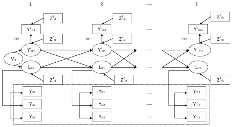
The DLTM-MHMM Modeling Framework.
In the process of fitting all models, two chains of 100,000 iterations were run with every 50th iteration being saved after a burn in of 50,000 iterations. The model convergence is assessed by the Gelman-Rubin statistic [16]. The main objectives in this application include: 1) exploring the risk factors for both the asthma transition process and misclassification probability, 2) conducting inference on the effect of real asthma state in the previous time period on lung function growth; and 3) estimating the effect of air pollution on respiratory health in children through the latent variable structure, based on the observed information on lung function growth and asthma state.
The results from fitting the proposed DLTM-MHMM for asthma and lung functions are summarized in Table 4. Children with severe wheezing were more likely to have asthma at baseline (Severe Wheezing: OR (95%CI)=6.1(1.84,19.89)). As age increased, children were less likely to become asthmatic (Age: OR (95%CI)=0.4 (0.17,0.79)). During the follow-up period, children with allergy or family asthma history were more likely to become asthmatic (Allergy: OR (95%CI)=2.9 (1.32,6.42); Family Asthma: OR (95%CI)=2.7 (1.21,6.11)). Besides the findings in both the prevalence and transition probabilities for asthma, the model provided us with new insight by enabling us to detect the factors associated with misclassification in asthma. Children with current wheezing but without asthma were more likely to misclassify themselves as having asthma (OR (95%CI)=2.6 (1.07,6.69)). Children whose parents had above high school education were more likely to correctly identifying having real asthma (OR (95%CI)=3.78 (1.19, 12.18)). The 95% credible interval for estimated variance of town-level random effect excluded the null (data not shown), which implies that it is appropriate to include random term model in modeling the asthma transition process.
Table 4.
Results of DLTM-MHMM in Southern California Children Health Study
| Effect Estimate (95% CI) | OR (95% CI) | |
|---|---|---|
| Prevalence Probability | ||
| Age | 0.29(-0.78,1.34) | 1.34(0.46,3.82) |
| Allergy | 0.88(-0.06,1.83) | 2.41(0.94,6.23) |
| Severe wheezing | 1.8(0.61,2.99) | 6.05(1.84,19.89) |
|
| ||
| Transition Probability | ||
| Age | -0.9(-1.75,-0.23) | 0.41(0.71,0.079) |
| Allergy | 1.07(0.28,1.86) | 2.92(1.32,6.42) |
| Family Asthma History | 0.98(0.19,1.81) | 2.66(1.21,6.11) |
| Latent lung functions transition effect on latent asthma | -0.17(-0.59,0.25) | 0.84(0.55,1.28) |
|
| ||
| Misclassification Probability | ||
| Current wheezing | 0.96(0.07,1.9) | 2.61(1.07,6.69) |
| Above HS | ||
| When Latent True Asthma=0 | -0.08(-0.9,0.8) | 0.92(0.41,2.23) |
| When Latent True Asthma=1 | 1.33(0.17,2.5) | 3.78(1.19,12.18) |
|
| ||
| Latent Lung Function Modeling | ||
| Age | 1.55(1.47,1.64) | — |
| Height | 28.08(25.7,30.47) | — |
| NO2 | -0.01(-0.02,0) | — |
| Latent lung function transition effect on itself | 0.87(0.83,0.92) | — |
| Latent asthma transition effect on latent lung function | -0.24(-0.4,-0.08) | — |
|
| ||
| Lung Function Measurements Modeling | ||
| Latent lung function effect on FEV1 | 0.07(0.07,0.07) | — |
| Latent lung function effect on FEF75 | 0.08(0.08,0.09) | — |
| Latent lung function effect on MMEF | 0.07(0.07,0.08) | — |
Note: In the prevalence and transition probability models, we also adjusted for gender, and race/ethnicity. Medication Use and FEV were adjusted in prevalence models. Transition Probability models were also adjusted for Ozone, number of sports and their interaction. In the misclassification probability models, we also adjusted for age and gender. Latent true asthma variable and its interaction with age were included in the misclassification probability model. Town-level random effect is included in the transition process. Town-level random effect is included in the transition process. Asthma state is set as an absorbing state. Gender is adjusted in the latent lung function models.
Latent lung function was significantly associated with real asthma state at previous time period (Effect Estimate (95%CI): -0.2 (-0.4,-0.08)) and previous lung function (Effect Estimate (95%CI): 0.9 (0.83, 0.92)). One appealing insight from using the proposed approach in this application was that it revealed increased percentage of children getting abnormal lung function level due to the occurrence of asthma in the previous time period. To our knowledge, the increased percentage of children getting abnormal lung function is usually calculated based on the observed lung function measurement, usually leading to the awkward situation where different lung function measurements in the same study could result in different estimated percentage. Using latent lung function level variables, which are fewer in number compared to the observed lung function measures, avoids this proliferation. Note that the posterior distribution of the latent lung function development variable Lij, given the latent lung function level Lij−1 and asthma state at previous time period, is assumed to follow the normal distribution with unit variance, for identifiability reasons, and could be interpreted as a z-score ranking the unobserved lung function level for children of a given asthma state. It is straightforward to utilize the normal cutoff value based on lower limits of normal method (LLN), which is recommended by the American Thoracic Society (ATS) and European Respiratory Society (ERS), to describe normal/abnormal lung function [29]. Based on LLN, the 5th percentile of posterior distribution of Lij when real asthma state at previous time period is defined as the cutoff point for children with given age, height, gender, air pollution level and lung function level at previous time period. If Lij is less than this cut-point, subject i at time period j has abnormal lung function level. In Figure 2, the posterior distribution of latent lung function level for children without asthma was drawn with the dashed curve. Without loss of generality, we set its posterior mean at zero. The vertical dash-dot line marks the location of the normal\abnormal cutoff point based on LLN. Because of the adverse effect of asthma, the posterior distribution of latent lung function level for children with asthma, which is drawn with a solid curve, had a location shift to the left with a size of -0.24. It is easy to see that the size of the shaded area at the left tail describes the increased percentage of children getting abnormal lung function level due to the occurrence of asthma in the previous time period. In our application, the estimated percentage increase of having abnormal lung function in children due to the onset of asthma in previous visit is 3% with 95% credible interval (1%, 5%).
Figure 2.

Comparison of Posterior Distribution for Lung Function by Asthma
The chronic effect of NO2 (based on multi-year average for 1994-2000) on latent lung function development was explored (Table 4). We found that NO2 is significantly associated with the latent lung function development (Effect Estimate (95%CI): -0.01 (-0.02, -0.004)). In terms of difference in the annual percentage growth rate from least to most polluted communities (range in NO2 across 12 communities is 36.8ppb), we found observed lung function measurements for children from the most polluted community are about 2~3% lower than those from the least polluted community (FEV1: 2.5% (2.4%, 2.6%), MMEF:3.2% (3.0%, 3.3%), FEF75: 2.7% (2.6%, 2.9%)). This finding was consistent with the report by Gauderman and others [24] and confirmed that in early childhood, exposure to NO2 was associated with reduced lung function growth.
6. Summary
We proposed a dynamic latent trait model with mixed hidden Markov (DLTM-MHMM) for jointly modeling longitudinal data with mixed outcomes from the exponential family and allowing for possible misclassification in categorical outcomes. The main advantages of this approach include 1) ability to model misclassification 2) ability to model mixed longitudinal outcomes 3) ability to model the autocorrelation and cross-correlation among latent variables using dynamic structure, and 4) ability to accommodate heterogeneity at different cluster levels.
This approach was illustrated by studying the effect of long term levels of ambient air pollution on children’s lung function growth and asthma state in the CHS. This joint modeling approach not only integrated prior well-known scientific evidence across various outcomes into one unified structure, but also provided some new insights and quantified the serial dependence features in asthma and lung function development through a dynamic transition process. While this study was motivated by the CHS, in which a battery of lung function development measurements and questionnaire-based asthma state at different ages were modeled to illustrate the utility of this approach, the proposed method has a much wider application and is amenable to any study with similar multi-level prospective design and potential misclassification in categorical outcomes.
Supplementary Material
Acknowledgments
We gratefully acknowledge important discussions with Drs. Jim Gauderman, Chih-Ping Chou, Duncan Thomas, Rob McConnell and Frank Gilliland.
Funding sources:
This work was supported by the NIEHS grants 5P30ES007048, 5P01ES011627 and 5P01ES009581; EPA grants R826708-01 and RD831861-01; NHLBI grants 5R01HL061768 and 5R01HL076647; CARB contract 94-331; and the Hastings Foundation.
References
- 1.Legler JM, Lefkopoulu M, Ryan LM. Efficiency and Power of Tests for Multiple Binary Outcomes. Journal of the American Statistical Association. 1995;90(430):680–693. [Google Scholar]
- 2.O’Brien PC. Procedures for Comparing Samples with Multiple Endpoints. Biometrics. 1984;40(4):1079–1087. [PubMed] [Google Scholar]
- 3.Pocock SJ, Geller NL, Tsiatis AA. The Analysis of Multiple Endpoints in Clinical Trials. Biometrics. 1987;43(3):487–498. [PubMed] [Google Scholar]
- 4.Sammel M, Lin X, Ryan L. Multivariate linear mixed models for multiple outcomes. Stat Med. 1999;18(17-18):2479–92. doi: 10.1002/(sici)1097-0258(19990915/30)18:17/18<2479::aid-sim270>3.0.co;2-f. [DOI] [PubMed] [Google Scholar]
- 5.Arminger G, Küsters U. Latent Trait Models With Indicators of Mixed Measurement Level. In: Langeheine R, Rost J, editors. Latent Trait and Latent Class Models. Plenum; New York: 1988. pp. 51–73. [Google Scholar]
- 6.Shah A, Laird N, Schoenfeld D. A Random-Effects Model for Multiple Characteristics With Possibly Missing Data. Journal of the American Statistical Association. 1997;92(438):775–779. [Google Scholar]
- 7.Roy J, Lin X. Latent Variable Models for Longitudinal Data with Multiple Continuous Outcomes. Biometrics. 2000;56(4):1047–1054. doi: 10.1111/j.0006-341x.2000.01047.x. [DOI] [PubMed] [Google Scholar]
- 8.Sammel MD, Ryan LM, Legler JM. Latent Variable Models for Mixed Discrete and Continuous Outcomes. Journal of the Royal Statistical Society: Series B (Statistical Methodology) 1997;59(3):667–678. [Google Scholar]
- 9.Moustaki I, Knott M. Generalized latent trait models. Psychometrika. 2000;65(3):391–411. [Google Scholar]
- 10.Miglioretti DL. Latent Transition Regression for Mixed Outcomes. Biometrics. 2003;59(3):710–720. doi: 10.1111/1541-0420.00082. [DOI] [PubMed] [Google Scholar]
- 11.Dunson DB. Dynamic Latent Trait Models for Multidimensional Longitudinal Data. Journal of the American Statistical Association. 2003;98(463):555–563. [Google Scholar]
- 12.Altman RM. Mixed Hidden Markov Models: An extension of the hidden Markov model to the longitudinal data setting. Journal of the American Statistical Association. 2007;102(477):201–210. [Google Scholar]
- 13.Zhang Y, Berhane K. Bayesian mixed hidden Markov models: a multi-level approach to modeling categorical outcomes with differential misclassification. Stat Med. 2014;33(8):1395–408. doi: 10.1002/sim.6039. [DOI] [PMC free article] [PubMed] [Google Scholar]
- 14.Garrett ES, Zeger SL. Latent Class Model Diagnosis. Biometrics. 2000;56(4):1055–1067. doi: 10.1111/j.0006-341x.2000.01055.x. [DOI] [PubMed] [Google Scholar]
- 15.Spiegelhalter DJ, Thomas A, B GN, Lunn D. WinBUGS Version 1.4 User Manual. MRC Biostatistics Unit. 2003 [Google Scholar]
- 16.Gelman A, Rubin DB. Inference from Iterative Simulation Using Multiple Sequences. Statistical Science. 1992;7(4):457–472. [Google Scholar]
- 17.Stephens M. Bayesian Mothods for Mixtures of Normal Distributions. University of Oxford; Oxford: 1997. [Google Scholar]
- 18.Sperrin M, Jaki T, Wit E. Probabilistic relabelling strategies for the label switching problem in Bayesian mixture models. Statistics and Computing. 2010;20(3):357–366. [Google Scholar]
- 19.Navidi W, et al. Design and analysis of multilevel analytic studies with applications to a study of air pollution. Environ Health Perspect. 1994;102(Suppl 8):25–32. doi: 10.1289/ehp.94102s825. [DOI] [PMC free article] [PubMed] [Google Scholar]
- 20.Navidi W, Lurmann F. Measurement error in air pollution exposure assessment. J Expo Anal Environ Epidemiol. 1995;5(2):111–24. [PubMed] [Google Scholar]
- 21.Peters JM, et al. A study of twelve Southern California communities with differing levels and types of air pollution. II. Effects on pulmonary function. Am J Respir Crit Care Med. 1999;159(3):768–75. doi: 10.1164/ajrccm.159.3.9804144. [DOI] [PubMed] [Google Scholar]
- 22.Peters JM, et al. A study of twelve Southern California communities with differing levels and types of air pollution. I. Prevalence of respiratory morbidity. Am J Respir Crit Care Med. 1999;159(3):760–7. doi: 10.1164/ajrccm.159.3.9804143. [DOI] [PubMed] [Google Scholar]
- 23.Gauderman WJ, et al. The effect of air pollution on lung development from 10 to 18 years of age. N Engl J Med. 2004;351(11):1057–67. doi: 10.1056/NEJMoa040610. [DOI] [PubMed] [Google Scholar]
- 24.Gauderman WJ, et al. Association between air pollution and lung function growth in southern California children. Am J Respir Crit Care Med. 2000;162(4 Pt 1):1383–90. doi: 10.1164/ajrccm.162.4.9909096. [DOI] [PubMed] [Google Scholar]
- 25.McConnell R, et al. Indoor risk factors for asthma in a prospective study of adolescents. Epidemiology. 2002;13(3):288–95. doi: 10.1097/00001648-200205000-00009. [DOI] [PubMed] [Google Scholar]
- 26.McConnell R, et al. Asthma in exercising children exposed to ozone: a cohort study. Lancet. 2002;359(9304):386–91. doi: 10.1016/S0140-6736(02)07597-9. [DOI] [PubMed] [Google Scholar]
- 27.McConnell R, et al. Prospective study of air pollution and bronchitic symptoms in children with asthma. Am J Respir Crit Care Med. 2003;168(7):790–7. doi: 10.1164/rccm.200304-466OC. [DOI] [PubMed] [Google Scholar]
- 28.Spiegelhalter DJ, et al. Bayesian measures of model complexity and fit. Journal of the Royal Statistical Society: Series B (Statistical Methodology) 2002;64(4):583–639. [Google Scholar]
- 29.Stanojevic S, et al. Reference ranges for spirometry across all ages: a new approach. Am J Respir Crit Care Med. 2008;177(3):253–60. doi: 10.1164/rccm.200708-1248OC. [DOI] [PMC free article] [PubMed] [Google Scholar]
Associated Data
This section collects any data citations, data availability statements, or supplementary materials included in this article.