Historical Evolution of Old-Age Mortality and New Approaches to Mortality Forecasting

Abstract

Knowledge of future mortality levels and trends is important for actuarial practice but poses a challenge to actuaries and demographers. The Lee-Carter method, currently used for mortality forecasting, is based on the assumption that the historical evolution of mortality at all age groups is driven by one factor only. This approach cannot capture an additive manner of mortality decline observed before the 1960s. To overcome the limitation of the one-factor model of mortality and to determine the true number of factors underlying mortality changes over time, we suggest a new approach to mortality analysis and forecasting based on the method of latent variable analysis. The basic assumption of this approach is that most variation in mortality rates over time is a manifestation of a small number of latent variables, variation in which gives rise to the observed mortality patterns. To extract major components of mortality variation, we apply factor analysis to mortality changes in developed countries over the period of 1900–2014.

Factor analysis of time series of age-specific death rates in 12 developed countries (data taken from the Human Mortality Database) identified two factors capable of explaining almost 94 to 99 percent of the variance in the temporal changes of adult death rates at ages 25 to 85 years. Analysis of these two factors reveals that the first factor is a “young-age” or background factor with high factor loadings at ages 30 to 45 years. The second factor can be called an “oldage” or senescent factor because of high factor loadings at ages 65 to 85 years. It was found that the senescent factor was relatively stable in the past but now is rapidly declining for both men and women. The decline of the senescent factor is faster for men, although in most countries, it started almost 30 years later.

Factor analysis of time series of age-specific death rates conducted for the oldest-old ages (65 to 100 years) found two factors explaining variation of mortality at extremely old ages in the United States. The first factor is comparable to the senescent factor found for adult mortality. The second factor, however, is specific to extreme old ages (96 to 100 years) and shows peaks in 1960 and 2000. Although mortality below 90 to 95 years shows a steady decline with time driven by the senescent factor, mortality of centenarians does not decline and remains relatively stable.

The approach suggested in this paper has several advantages. First, it is able to determine the total number of independent factors affecting mortality changes over time. Second, this approach allows researchers to determine the time interval in which underlying factors remain stable or undergo rapid changes. Most methods of mortality projections are not able to identify the best base period for mortality projections, attempting to use the longest-possible time period instead. We observe that the senescent factor of mortality continues to decline, and this decline does not demonstrate any indications of slowing down. At the same time, mortality of centenarians does not decline and remains stable. The lack of mortality decline at extremely old ages may diminish anticipated longevity gains in the future.

Introduction

Population aging is a global phenomenon that is particularly expressed in industrialized countries. The proportion of older people in these countries grows now at an accelerated pace, mainly due to increasing longevity. Population aging is expected to continue over the next few decades, eventually leading to a global convergence in the proportion of older people. Although fertility decline was the main cause of population aging in the past, the process of population aging in contemporary societies is determined by declining mortality at older ages. Thus, mortality studies and projections for older ages are particularly important for making accurate demographic forecasts of population aging.

This paper is focused on mortality changes at older ages because these changes are now the main driving force behind both increases in life expectancy and population aging. In this paper, we present some new approaches to mortality forecasts and population projections at older ages.

Using Parametric Models (Mortality Laws) for Mortality Projections

Parametric models of mortality represent a useful tool in demographic and actuarial projections of mortality. One of the first and most successful attempts to express the dependency between mortality and age mathematically was that of the English actuary Benjamin Gompertz (1825):

$${\mathrm{\mu }}_x=R_{0}exp(\alpha x)$$ (1)

where μ_x is the force of mortality (hazard rate) at age x, and α and R₀ are the slope and level parameters of the equation (Bongaarts 2005). This formula, which describes the mortality of people older than 20, was called the Gompertz law, and its parameters were named the Gompertz parameters. Subsequently, the Gompertz law began to be used widely for describing the mortality of laboratory animals (Gavrilov and Gavrilova 1991).

In his work, Gompertz noted that, in addition to the mortality that grows exponentially with age, there can also exist a component of mortality that is independent of age: “It is possible that death may be the consequence of two generally coexisting causes: the one chance, without previous disposition to death or deterioration, or increased inability to withstand destruction” (Gompertz 1825). However, for the analysis of the life tables that were then available, Gompertz considered it possible to restrict himself solely to the exponential component of mortality. Not until 35 years later did another actuary, William Makeham, add the age-independent component to the Gompertz formula (Makeham 1860). This component, usually denoted by the letter A, received the name of the Makeham parameter (Gavrilov and Gavrilova 1991). Adding A resulted in the formula we now know as the Gompertz-Makeham law:

$${\mathrm{\mu }}_x=A+R_{0}exp(\alpha x)$$ (2)

We call A, the age-independent component of mortality, the “background component” of mortality, in analogy with background radiation (Gavrilov and Gavrilova 1979, 1991). The second term of this equation is the age-dependent component of mortality (Gavrilov and Gavrilova 1979), which we call the “senescent component” of mortality, as suggested by Wilmoth (1997).

The Gompertz-Makeham formula describes the life span distributions of a wide variety of biological species—drosophila, mosquitoes, flour beetles, mice, rats, horses, mountain sheep and humans (Gavrilov and Gavrilova 1991). There are some reports that the competing Weibull formula (power law) fits data better than the Gompertz formula. These reports are usually based on analysis of a few life tables for populations of small size (often less than 100 animals). Our comparative study of Weibull and Gompertz models using data for 260 human life tables and 129 life tables for fruit flies (including 15 life tables with initial population size of 1,000 or more animals) demonstrated that, on average, the Gompertz-Makeham law fits mortality at adult ages better than the Weibull-Makeham law (Gavrilov and Gavrilova 1991), although in some rare cases, the Weibull formula shows a better fit of mortality data.

Subsequently, there were many attempts to modify the Gompertz law. The most common way of modifying the Gompertz function is to use what are called logistic equations. The earliest such formula was proposed by Perks, and the latest and the most widely used one was proposed by Kannisto (1994) and is called a Kannisto formula:

$${\mathrm{\mu }}_x=\frac{Bexp(\alpha x)}{1+Bexp(\alpha x)}$$ (3)

The formulas 1-3 listed above are applicable to the mortality of adult populations (usually above age 20 years). There were also attempts to describe mortality in the entire age interval; these included the Heligman-Pollard (Heligman and Pollard 1980) and Siler (Siler 1979) formulas.

Parametric formulas can be used in population projections; this requires analyzing historical trends of their parameters. For example, in 1979, during an analysis of the historical changes in the mortality of the Swedish male population, it was found that the age-dependent component of mortality in the Gompertz-Makeham formula demonstrates surprising historical stability despite rapid decline in age-independent mortality, that is, the Makeham term (Gavrilov and Gavrilova 1979). Further more careful investigation confirmed the validity of this phenomenon (Gavrilov and Gavrilova 1991; Gavrilov at al. 1983), and the study of historical time series of mortality for 17 countries permitted the conclusion that it was quite general in character (Gavrilov and Gavrilova 1991). Figure 1 shows changes in total, background and senescent mortality for Swedish males. It can be seen that the background component of mortality is the only mortality component, which has significantly changed over the studied period (1900–1970). The senescent mortality (and two Gompertz parameters) turn out to be practically unchanged, despite the sharp fall in total mortality in the 20th century. We observe that the substantial decline in mortality rates in Sweden at the beginning of the 20th century can be explained by a decrease in the Makeham component, while the Gompertz component remained virtually constant during the same period. In the 1960s, as the Makeham component had almost reached zero, it became foreseeable that the rapid decline in mortality rates would come to an end. And this is what happened, in fact, in the 1960s (Gavrilov et al. 1983).

Fig. 1. Historical Changes of Age-Independent (Background) and Age-Dependent (Senescent) Mortality, per 1,000, for 40-Year-Old Swedish Males.

Key

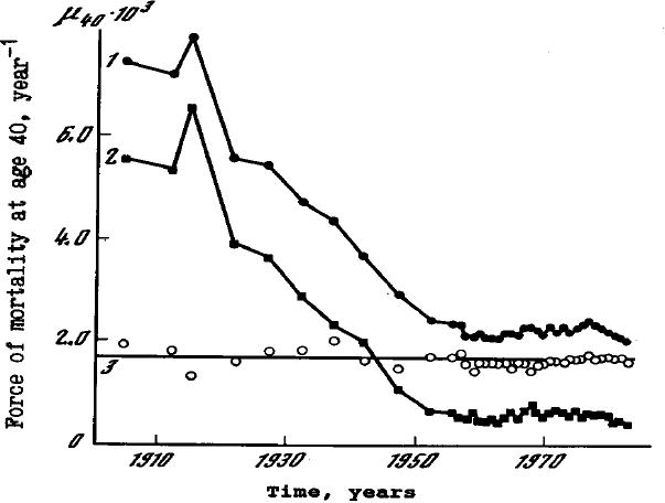
1. Total (observed) mortality at age 40, based on official Swedish life tables
2. Background mortality component, calculated on the basis of the Gompertz-Makeham formula
3. Senescent mortality component at age 40, calculated on the basis of the Gompertz-Makeham formula

Source: Gavrilov et al. 1983.

Thus, based on the observation of the mortality tables for the first half of the 20th century, it was possible to predict a “biological limit” to the force of mortality. For example, at the beginning of the 20th century, total mortality was substantially higher in Norway than in Denmark. However, based on the observation that the Gompertz component was considerably lower in Norway, we were able to predict a reversal in the trend as the Makeham component declines. This is exactly what happened (Gavrilov and Gavrilova 1991). Similarly, in Italy, the mortality rates of men and women were virtually identical at the beginning of the 20th century, but the biological limit for women was lower, due to the lower corresponding Gompertz component. Based on data from the beginning of the 20th century, we were able to predict that eventually, women's mortality would become lower than male mortality (Gavrilov and Gavrilova 1991). However after the 1960s, new, unexpected trends in mortality have started. These trends were not well visible at the time of this study, although some indications of further mortality decline have already been noticed (Gavrilov and Gavrilova 1991; Gavrilov and Nosov 1985).

Later Bongaarts developed further the method based on studying historical trends of Gompertz-Makeham parameters, suggesting the use of a logistic formula for mortality forecasting (Bongaarts 2005). This modification was reasonable because mortality rates for period life tables in the Human Mortality Database (used in his study) were fitted by a logistic formula after the age of 85 years (Wilmoth et al. 2007). His study analyzed historical trends in the interval 1950–2000 for 14 countries and confirmed a decline of the background mortality and stability of the slope parameter in the Gompertz term found in the previous studies. Due to the limited number of life tables (no life tables before 1950 were used), this study could not demonstrate the full scale of decline in the background mortality during the first half of the 20th century. However, this study revealed another interesting regularity that could not be fully analyzed in the past: decline in the pre-exponential multiplier of senescent mortality. The decline of this parameter (which Bongaarts called the level parameter) in conjunction with the stability of the slope parameter in the Gompertz term means that the senescent component of mortality in developed countries undergoes a parallel shift in semilog coordinates over time. This pattern of mortality change was called a shifting logistic model (Bongaarts 2005). Based on this mortality pattern, Bongaarts suggested a new approach to mortality projections. This approach is based on estimating parameters of the logistic formula for a number of years and extrapolating the values of three parameters—background mortality and two parameters of senescent mortality— to the future (Bongaarts 2005, 2009).

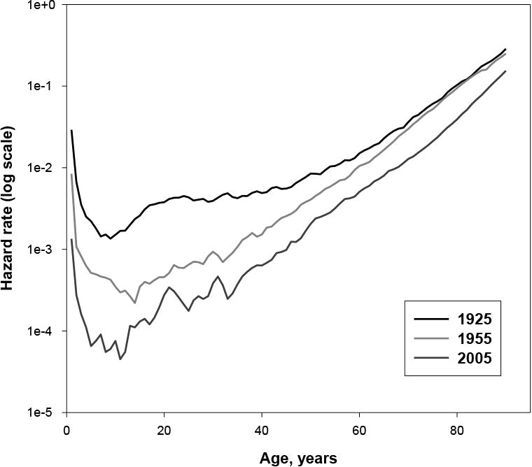
Figure 2 illustrates the two phases of mortality decline in the 20th century. When we analyze mortality data on a larger time scale, we observe a decline of mortality in all age groups between 1925 and 1955, except for the elderly, where death rates remained relatively constant. Note that mortality trajectories for 1925 and 1955 are close to each other at older ages, which corresponds to the stability of the senescent mortality during the first half of the 20th century. After the 1950s, the parallel shift of mortality has been observed, which corresponds to the model proposed by Bongaarts (for example, compare mortality trajectories for 1955 and 2005).

Fig. 2. Changing Patterns of Mortality Decline for Swedish Females.

In addition to the approach based on the background and senescent mortality, there is another way of mortality partitioning. In 1952, Jean Bourgeois-Pichat attempted to predict population mortality, using the idea of endogenous and exogenous causes of death (Bourgeois-Pichat 1952). In the exogenous causes of death he included infectious and parasitic diseases, respiratory diseases, accidents, poisonings and violence. The endogenous causes of death included malignant neoplasms, circulatory diseases and the remaining causes of death (Bourgeois-Pichat 1952). In Bourgeois-Pichat's opinion, the evolution of human mortality can be likened “to the erosion of soil composed of two kinds of rock: soft rock and hard rock.” At first, the “soft rock” is quickly eroded (exogenous causes of death); then the “hard rock” slowly erodes (endogenous causes of death). On the basis of these ideas, it was predicted that medical advances in eliminating the exogenous causes of death would lead to the endogenous causes of death coming to the fore. Thus, Bourgeois-Pichat formulated “the concept of a temporary limit on mortality decline” and even calculated the level of this “temporary limit” for each age, calling it “the biological limit of mortality decline” (Bourgeois-Pichat 1952; 1979). Later Carnes and Olshansky developed this approach further, suggesting so-called biologically motivated partitioning of mortality into extrinsic and intrinsic mortality based on cause-of-death information (Carnes and Olshansky 1997). Information on causes of death is used sometimes in actuarial practice for making mortality projections, although these projections usually underestimate future mortality decline.

Mortality partitioning proved to be a useful tool for mortality projections in the past, when background mortality (analog of extrinsic mortality) was high, but this approach is less useful now, when background mortality is close to zero and does not change significantly over time. In addition to that, in some cases, it is simply impossible to establish whether death is exogenous or endogenous. For example, a patient may be suffering from several diseases, none of which alone would lead to death but which are lethal in combination. So this approach has a limited applicability in demographic practice now.

Despite the usefulness of parametric approach to mortality projections, it has serious limitations. The main limitation is a dependence on the particular formula, which makes this approach too rigid for responding to possible changes in mortality trends and fluctuations. In the next section, we consider some methods of mortality projections based on nonparametric approaches.

Nonparametric Approach to Mortality Projections

One of the most widely used methods of mortality projections in demography and actuarial science today is the Lee-Carter method (Lee and Miller 2001; Lee and Carter 1992). Its success stemmed from the shifting model of mortality decline observed for industrialized countries during the last 30 to 50 years. The Lee-Carter method is applied to the logarithm of mortality and is based on the following formula for hazard rate, or central death rate (Lee 2000):

$$ln({\mathrm{\mu }}_{x,t})=\mathrm{a}(x)+b(x)k(t)$$ (4)

where a(x), b(x) and k(t) are parameters to be estimated. This model does not produce a unique solution, and Lee and Carter suggested applying the following constraints (Lee 2000; Lee and Carter 1992):

$$\sum _t\mathrm{k}(t)=0;\sum _x\mathrm{b}(x)=1$$ (5)

The first constraint implies that the parameter a(x) is an empirical average of the logarithm of mortality at age x over time. In the first stage of the Lee-Carter method, coefficients a(x) and b(x) are estimated. In the second stage, the empirical values of k(t) coefficients are estimated using the following formula (Lee 2000):

$$D_t=\sum exp(a_x+b_x{k}_t)N_{x,t}$$ (6)

where D_t is total number of deaths in year t, and N_xt is the population aged x in year t.

The empirical time series of k coefficients can be extrapolated from the base period to the future, which is essentially a linear extrapolation.

Note that the Lee-Carter method is modeling logarithms rather than absolute values of mortality and hence is based on a multiplicative model of mortality change over time (rather than an additive one, as in the case of the Gompertz-Makeham model). However, the Lee-Carter model is not based on any particular parametric formula and allows researchers to make a compact description of a large set of mortality data without excessive loss of information. In contrast to aggregated indicators such as life expectancy, the knowledge of the Lee-Carter model parameters allows researchers to reconstruct values of age-specific mortality rates and their temporal evolution with reasonable accuracy.

One limitation of this method is related to the assumption that historical evolution of mortality at all age groups is driven by one factor only—parameter b (Lee 2000). However, a factor analysis of mortality evolution (see the appendix for details) found that this approach turns out to be overly simplistic (Gavrilov and Gavrilova 1991; Gavrilov and Nosov 1985). For example, factor analysis of mortality dynamics over the period of 1900–2014 in developed countries found that at least two time-dependent factors are responsible for the observed decline of mortality (younger age groups have a different factor of mortality decline compared with older groups). A one-factor model could be applicable to earlier historical periods (before the 1950s), when a decline in mortality rates was driven mainly by a decrease in the background mortality, that is, the Makeham parameter of the Gompertz-Makeham law (Gavrilov and Gavrilova 1991; Gavrilov et al. 1983). It is obvious that the Lee-Carter model is not well applicable to mortality modeling during the period 1900–1950 because of the additive rather than multiplicative model of mortality decline during this time.

To overcome this limitation of the one-factor model of mortality and to determine the true number of factors underlying mortality changes over time, we conducted a factor analysis of mortality over the period 1900–2014 (see the appendix for more detail). We used the so-called P-technique of factor analysis when the analysis occurs across different time points or observations (values of hazard rates at different years) for ages 25 through 85 (Uberla 1977). We applied a factor analysis procedure with the promax rotation method using the Stata statistical package, release 13. Data on men and women were analyzed separately. The analyses were conducted for 12 industrialized countries with sufficiently long time series of mortality data.

We identified two factors capable of explaining almost 98 percent of the variance in the temporal changes of hazard rates (see Table 1). Thus, for a more accurate description of mortality evolution, the following model would be preferable:

Table 1. Results of Applying Factor Analysis to Adult Mortality Data of Swedish Men and Women, 1900–2014.

Factor	Eigenvalue	Proportion of Variance Explained	Cumulative Proportion of Variance Explained
Men
Factor 1	52.741	0.8733	0.8733
Factor 2	5.961	0.0987	0.9720
Factor 3	0.619	0.0103	0.9822
Factor 4	0.186	0.0031	0.9853
Factor 5	0.080	0.0013	0.9866
Women
Factor 1	55.097	0.9079	0.9079
Factor 2	4.691	0.0773	0.9852
Factor 3	0.304	0.0050	0.9902
Factor 4	0.115	0.0019	0.9921
Factor 5	0.044	0.0007	0.9928

Note: Variables included hazard rate values for ages 25–85 years; factor analysis used promax rotation.

$$\mathrm{\mu }(x,t)=a_0(x)+a_1(x)F_1(t)+a_2(x)F_2(t)$$ (7)

where x is age; t is time; α(x), α₁(x) and α₂(x) are three sets of parameters depending on age only; and F₁(t) and F₂(t) are two sets of parameters depending on time only (sets of coefficients determined by factor analysis models).

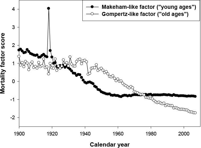
By studying the variation of these factors over time, we noted that the first factor— comparable to the Makeham component and observed in the “young” population (see Table 2)—declined from the beginning of the century. The second factor—comparable to the senescent mortality and chiefly concerning the “old ages” population—remained remarkably stable over the period 1900–1950 (see Figures 3 and 4). Without more recent data, we might predict continued historical stability of this factor. However, a radical change has occurred after the 1950s, and mortality has begun to decline among older people while the mortality of the younger age groups has already reached very low levels close to zero. Thus, factor analysis of the time series of mortality confirms the preferential reduction in the mortality of old people in recent years. Also note that for males, the senescent factor started its rapid decline significantly later than for females. Information about senescent and background factors for all countries is presented in Table 3. Note that for some countries with longer time series starting in 1900, the background factor explains the variation of mortality better than the senescent factor.

Table 2. Factor Analysis of Historical Changes of Mortality for Swedish Women*.

Mortality Rate at Given Age, Years	Factor Loadings for Factor 1	Factor Loadings for Factor 2
25	−0.0456	1.0209
35	0.0648	0.9462
45	0.3166	0.7415
55	0.5165	0.5528
65	0.7677	0.2852
75	0.9448	0.0686
85	0.9908	−0.0110

Note: Rotated factor loadings (for hazard rates at selected ages) for the first two factors after applying factor analysis to historical mortality changes for Swedish women.

Fig. 3. Time Dependence of Factor Scores for “Young-Age” and “Old-Age” Factors for Swedish Males.

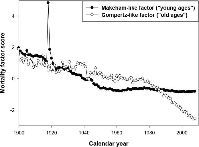
Table 3. Results of Applying Factor Analysis to Adult Mortality Data of 12 Countries.

Country	Sex	Time Range	Senescent Factor		Background Factor		Cumulative Proportion of Variance Explained by Two Factors
			Eigenvalue	Proportion of Variance Explained	Eigenvalue	Proportion of Variance Explained
Australia	M	1921–2011	50.59	0.8354	8.12	0.1341	0.9694
	F		56.18	0.9251	3.49	0.0574	0.9825
Canada	M	1921–2011	52.95	0.8729	5.80	0.0956	0.9685
	F		57.89	0.9512	2.28	0.0375	0.9887
Denmark	M	1900–2014	51.05	0.8522	5.04	0.0841	0.9364
	F		3.52	0.0582	55.22	0.9138	0.9720
England & Wales	M	1900–2013	49.16	0.8076	8.67	0.1424	0.9500
	F		2.13	0.0350	57.74	0.9476	0.9826
Finland	M	1900–2012	48.47	0.8069	8.15	0.1357	0.9426
	F		3.38	0.0558	55.97	0.9248	0.9848
France	M	1900–2014	50.82	0.8343	9.04	0.1485	0.9828
	F		58.34	0.9573	1.99	0.0327	0.9900
Italy	M	1900–2012	51.76	0.8502	6.70	0.1100	0.9602
	F		57.80	0.9482	2.70	0.0443	0.9925
Netherlands	M	1900–2012	54.92	0.9055	3.36	0.0554	0.9609
	F		2.96	0.0487	57.00	0.9368	0.9855
Norway	M	1900–2014	50.13	0.8324	7.48	0.1243	0.9567
	F		4.38	0.0721	55.10	0.9070	0.9790
Spain	M	1908–2014	3.39	0.0557	53.84	0.8844	0.9401
	F		3.45	0.0567	53.97	0.8857	0.9424
Sweden	M	1900–2014	52.74	0.8733	5.96	0.0987	0.9720
	F		55.10	0.9079	4.69	0.0773	0.9852
United States	M	1933–2013	54.90	0.9004	5.04	0.0826	0.9830
	F		58.89	0.9656	1.73	0.0284	0.9940

Note: Variables included hazard rate values for ages 25–85 years; factor analysis used promax rotation.

Figure 5 shows time trends of background and senescent mortality factors in Italy and France. Note the peaks of background mortality in 1918 (Spanish flu epidemics) and in the 1940s (World War II). The senescent mortality factor starts to decline later for men than for women. It is interesting that French women represent the only population where the senescent factor started to decline before World War II (in 1910). Figure 6 compares time trends of background and senescent mortality factors in Canada and the United States. The background factor shows rapid decline between 1940 and 1960 with little changes afterward. Note a peak in the background factor in the 1980s for the U.S. men; this apparently reflects mortality related to the AIDS epidemic. Again, the decline of the senescent factor started later for men than for women.

Fig. 5. Time Trends of Factor Scores for Senescent and Background Mortality Factors: Italian and French Men and Women.

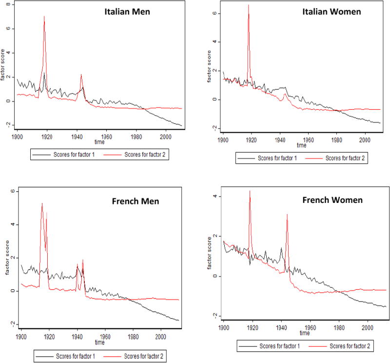
Note: The senescent factor is shown in black, and the background factor in red.

Fig. 6. Time Trends of Factor Scores for Senescent and Background Mortality Factors: Canadian and U.S. Men and Women.

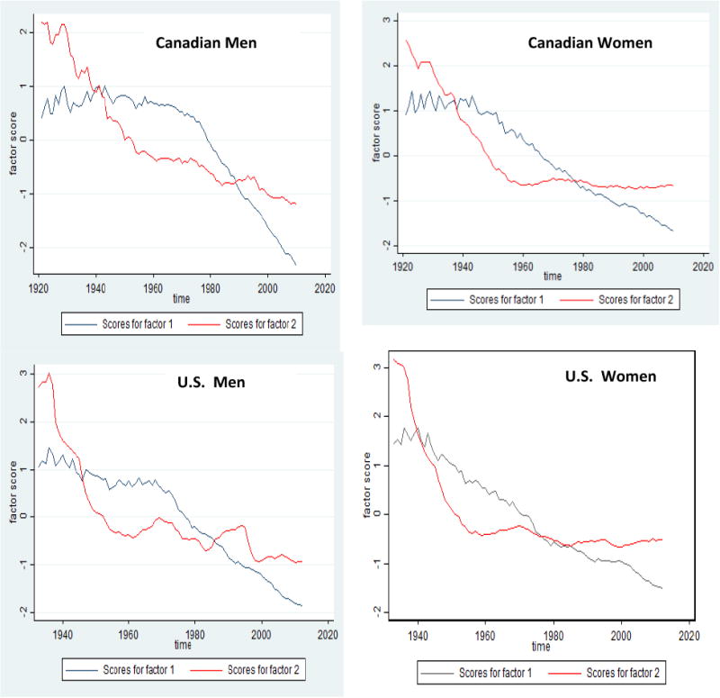
Note: The senescent factor is shown in black, and the background factor in red.

Observations made before 1950 enrich the historical data as a whole but are liable to distort the results of mortality projections. For mortality forecasts, it is better to use more recent data, which take account of the change in the patterns of mortality decline. What conclusions may be drawn at this point? In the past, it was possible to argue that there was a biological limit underlying the observed mortality rate. We have observed, however, that these limits can be pushed back, thanks to technological or medical progress. Although it is equally impossible to conclude that the mortality force is tending toward zero, the short-term trend is clearly oriented downward.

The approach based on the factor analysis has several advantages. First, it is able to determine the number of factors affecting mortality changes over time. Second, this approach allows researchers to determine the time interval in which underlying factors remain stable or undergo rapid changes. For example, Figures 3 through 6 clearly demonstrate that the senescent factor was relatively stable in the past but now is rapidly declining for both men and women. However, this rapid decline started almost 30 years later in men than in women. Most methods of mortality projections are not able to identify the best base period of time for mortality changes that should be extrapolated into the future. For example, the Lee-Carter method suggests using the longest possible time interval. It is clear that such an approach will not bring the most accurate mortality forecast. Using the results of factor analysis, we may determine the best starting year for mortality projections (see Table 4). For example, the period 1980–2014 is a useful base period of mortality extrapolation for Swedish men. After 1980, the senescent factor demonstrates a stable linear decline, and it is reasonable to suggest that this decline will continue into the foreseeable future.

Table 4. Rate of Decline for the Senescent Factor in the Studied Countries.

Country	Sex	Year When Senescent Factor Started to Decline	Rate of Decline, per Year [95% CI]
Australia	M	1970	−0.075 [−0.078, −0.072]
	F	1970	−0.048 [−0.050, −0.046]
Canada	M	1978	−0.075 [−0.076, −0.073]
	F	1950	−0.041 [−0.043, −0.039]
Denmark	M	1990	−0.099 [−0.105, −0.093]
	F	1950	−0.029 [−0.031, −0.027]
England & Wales	M	1970	−0.053 [−0.054, −0.051]
	F	1950	−0.039 [−0.041, −0.038]
Finland	M	1970	−0.058 [−0.059, −0.056]
	F	1970	−0.042 [−0.045, −0.040]
France	M	1970	−0.036 [−0.037, −0.035]
	F	1910	−0.031 [−0.032, −0.030]
Italy	M	1980	−0.056 [−0.058, −0.053]
	F	1950	−0.031 [−0.033, −0.030]
Netherlands	M	1978	−0.071 [−0.076, −0.065]
	F	1950	−0.030 [−0.031, −0.028]
Norway	M	1980	−0.104 [−0.111, −0.099]
	F	1960	−0.045 [−0.048, −0.043]
Spain	M	1978	−0.041 [−0.043, −0.039]
	F	1978	−0.041 [−0.043, −0.039]
Sweden	M	1980	−0.073 [−0.075, −0.071]
	F	1950	−0.038 [−0.039, −0.036]
United States	M	1970	−0.057 [−0.059, −0.055]
	F	1950	−0.039 [−0.041, −0.037]

Note: Rate of decline corresponds to the slope coefficient of the linear regression model for the senescent factor on time.

Taking into account the shifting model of mortality change, it is reasonable to conclude that mortality after 1980 can be modeled by the following log-linear model with a similar slope for all adult age groups:

$$ln({\mathrm{\mu }}_{x,t})=\mathrm{a}(x)-kt$$ (8)

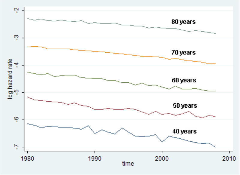
Figure 7 illustrates the validity of the suggested model for Swedish men. Note that the logarithm of mortality declines linearly in all observed age groups with the same linear slope. Similar regularity is observed for other studied populations.

Fig. 7. Linear Changes of Logarithm of Hazard Rate at Different Ages after 1980 for Swedish Men.

These results also suggest that the Lee-Carter method of mortality projections is better applied using a base period determined by the factor analysis of mortality change.

Mortality Changes at Extreme Old Ages

We demonstrated that contemporary mortality at adult and old ages can be modeled by simple one-factor model. However, mortality at extreme old ages may have different latent factors affecting its changes over time. For this reason, we applied the P-technique of factor analysis again to age-specific death rates for ages 65 through 100 years. We applied the factor analysis procedure with promax rotation method to the U.S. time series data for men and women separately. We identified two factors capable of explaining 96 to 97 percent of the variance in the temporal changes of death rates after age 65.

By studying time trends in these factors (Figure 8), we noted that the first factor is comparable to the senescent mortality and explains 84 to 86 percent of mortality variation. For U.S. women, this factor shows a temporary plateau during the 1990s but now continues to decline. The senescent factor has the highest factor loadings for ages between 65 and 93 years for men and between 65 and 96 years for women. The second factor, explaining 11 to 12 percent of mortality variation, has the highest loadings at ages 95 to 100 years and hence can be called the extreme old factor of mortality. In the United States, this factor shows peaks in 1960 and 2000, which are closely related to mortality changes at extremely old ages.

Fig. 8. Time Trends of Factor Scores for Old-Age Factors for U.S. Men and Women.

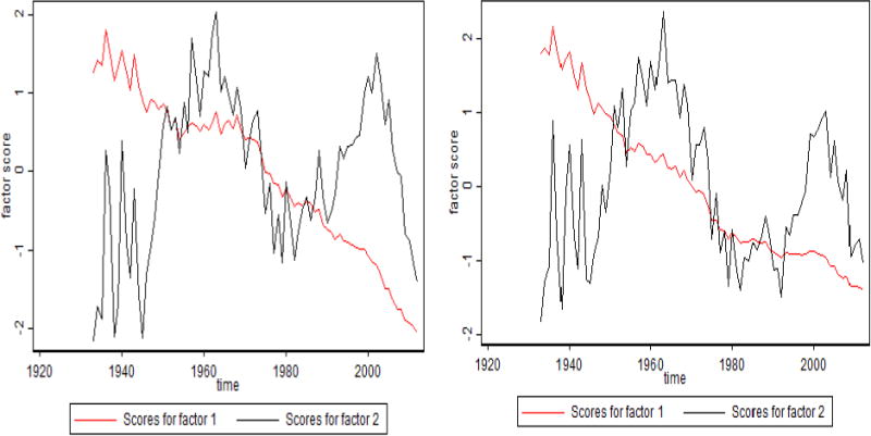
Note: The oldest-old factor is shown in black, and the old-age factor is shown in red.

It is noteworthy that mortality of centenarians in the United States does not demonstrate an obvious tendency to decline over time, in contrast to mortality at younger ages (see Figure 9). This stability of mortality of centenarians over time was first observed for Swedish centenarians (Drefahl et al. 2012) and recently was reported for centenarians in the United Kingdom (Continuous Mortality Investigation 2015). In this study, we observe the same phenomenon for centenarians in the United States. More detailed analysis of mortality trends for very old persons aged 92 to 102 years revealed more complex mortality behavior over time, compatible with the behavior of the extreme-old mortality factor (Figure 10).

Fig. 9. Time Trends of Old-Age Mortality for U.S. Men and Women.

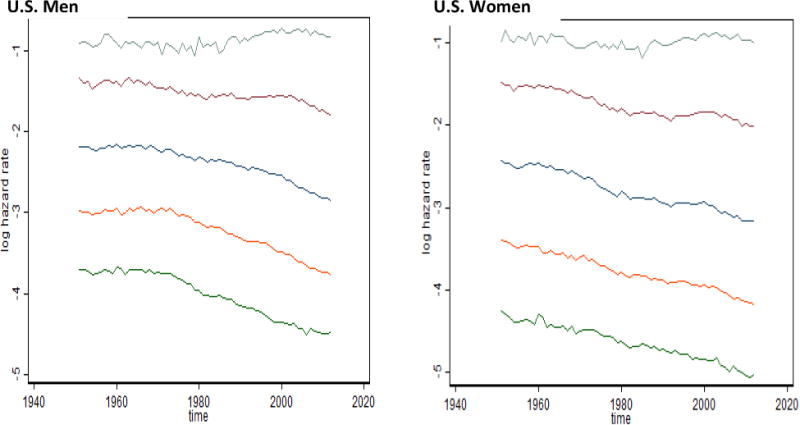
Key: From top to bottom: Mortality at ages 100, 90, 80, 70 and 60 years

Fig. 10. Time Trends of Extreme Old-Age Mortality for U.S. Men and Women.

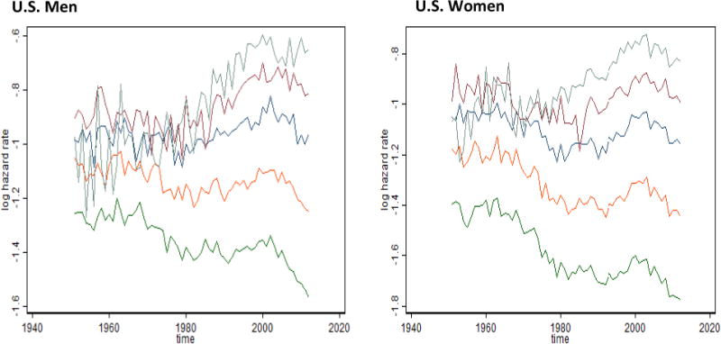
Key: From top to bottom: Mortality at ages 102, 100, 98, 95 and 92 years.

Making Mortality Forecasts Using Information From the Observed Phenomena

The factor analysis of mortality changes indicates that the age-dependent (senescent) mortality continues to decline and this decline does not demonstrate any indications of slowing down (Figures 3 through 6). This observation means that the traditional Lee-Carter approach can be used for mortality forecasting. The study of mortality changes using factor analysis demonstrates that mortality trends after 1980 can be continued beyond 2014 for both men and women. As can be seen from Figure 7, logarithms of mortality after 1980 for Swedish men show practically linear decline over time with similar slope for the studied ages. We can use this property to model mortality decline after 2015, assuming the same rate of mortality changes (in a log scale) for different ages.

In the case of other countries, the base period for mortality forecast can be specific for each particular country and can be determined empirically. Table 4 shows that during the last 40 years, the rate of decline for the senescent factor is higher for men than for women. On a log scale, mortality declines in a linear fashion in all adult age groups. It is possible to calculate the rate of mortality decline for each particular country. Based on the observed mortality trends, the mortality of Swedish males declines by 2 percent per year on average, while mortality of Swedish female declines by 1 percent per year. These gender differences in the rate of mortality decline over the last three decades are apparently responsible for the decreasing gender gap in life expectancy observed now in the majority of developed countries (Glei and Horiuchi 2007).

Another observation affecting mortality forecasts is the absence of time-dependent mortality decline among persons older than 96 to 100 years. This observation should be taken into account when making mortality forecasts.

Conclusions

We demonstrated that the use of factor analysis allows us to reveal factors that drive mortality changes over time. Our analyses show that the two-factor pattern of mortality decline in the 20th century is observed for the majority of industrialized countries. During the last 40 years, adult mortality decline can be described by only one factor, and this phenomenon justifies the use of the one-factor Lee-Carter method of mortality forecasting. Our approach allows researchers to find the most optimal base period for mortality forecasting when the background factor remains constant and the senescent factor shows steady decline over time. This one-factor model, however, cannot be applied to extreme old ages (over 96 years) when mortality is driven by its own factor with specific behavior over time.

This study assumes that no changes in mortality patterns are expected in the future. This is most likely an overly simplistic view. Old-age mortality may be affected by different tendencies in the future. On the one hand, an anticipated longevity revolution and new anti-aging technologies are able to slow down the aging process, resulting in a significant decline of mortality at older ages (Illes, de Grey and Rae 2007). On the other hand, epidemics of obesity and diabetes in developed countries may slow down future mortality decline (Olshansky et al. 2005). These multidirectional trends will shape the pattern of mortality changes in the coming decades and affect population aging in industrialized countries. Lack of mortality decline at extremely old ages may also diminish anticipated longevity gains in the future.

Appendix: Application of Factor Analysis to Mortality Changes Over Time

Factor analysis is a useful statistical method for data compression. Factor analysis originated with the work of Spearman and finds a small number of common latent variables (factors) that linearly reconstruct a larger number of original variables (Kerlinger 1986; Stata Corp. 2009). This approach may be useful for reducing the array of mortality rates for a large number of age groups. In this case, the standardized values of mortality rate (or hazard rate) at age x and time t can be presented as follows (Stata Corp. 2009):

$$\mathrm{\mu }(x,t)=a_1(x)F_1(t)+a_2(x)F_2(t)+\dots +a_q(x)F_q(t)+\mathrm{e}(x,t)$$

Where a_k(x) is the set of linear coefficients called factor loadings, F_k(t) is the kth common factor for observation at time t, and e(k, t) is similar to a residual error term. Such model has an infinite number of solutions, and various constraints are introduced to make this model determinate. To produce results in a form that is easier to interpret, one must rotate factor matrices (Kerlinger 1986). A rotation that requires the factors to remain uncorrelated is an orthogonal rotation, while others are oblique rotations (Stata Corp. 2009). In our analyses, we applied the oblique promax rotation method, since it does not impose additional constraints of orthogonality on factors.

The initial data set for factor analysis of mortality in our study is represented by a set of period life tables taken from the Human Mortality Database (2015). Data were analyzed separately for men and women. We used age-specific period death rates as empirical estimates of hazard rates for ages 25 to 85 years. Factor analysis was applied to an array of age-specific values of hazard rates for years from 1900 to 2014 (when available). We applied the so-called P-technique of factor analysis, where values of hazard rates at different points of time were considered as observations while hazard rate values at different ages were considered as variables. Table 1 shows eigenvalues and percent of explained mortality variation for the top five factors for Swedish data. Table 3 shows eigenvalues and percent of explained mortality variation for the top two factors for all 12 studied countries.

It is a common practice in statistics to leave factors with eigenvalues greater than 1 for further analyses. Note that the first two factors explain more than 97 percent of the historical variation in mortality in the case of the Swedish data (Table 1). Table 2 shows the values of rotated factor loadings (for hazard rates at selected ages) for the first two factors in the case of Swedish women. It is clear from Table 2 that the second factor is a “young-age” or background factor because of very high factor loadings for mortality rates at ages 25 to 45 years. The first factor can be called an “old-age” or senescent factor because of high factor loadings for mortality rates at ages 65 to 85 years. As follows from Figure 4, the first factor (corresponding to background mortality) demonstrated rapid decline during the period 1900–1950. Its effect can be illustrated by Figure 2 (mortality curves for 1925 and 1955). Note that the main changes from declining background mortality are observed at younger ages, while mortality at older ages remains relatively stable. Decline in the senescent factor happened after the 1970s (see Figure 4), and the effect of this decline on mortality is clear when mortality data for 1955 and 2005 are compared (Figure 2). Taking into account that Figure 2 shows mortality trajectories in semilog scale, it is obvious that absolute changes in mortality during the 1955–2005 period were the highest at older ages.

Fig, 4. Time Dependence of Factor Scores for “Young-age” and “Old-Age” Factors for Swedish Females.

References

- Bongaarts J. Long-Range Trends in Adult Mortality: Models and Projection Methods. Demography. 2005;42(1):23–49. doi: 10.1353/dem.2005.0003. [DOI] [PubMed] [Google Scholar]
- Bongaarts J. Trends in Senescent Life Expectancy. Population Studies. 2009;63(3):203–213. doi: 10.1080/00324720903165456. [DOI] [PMC free article] [PubMed] [Google Scholar]
- Bourgeois-Pichat J. Essai sur la mortalite biologique de l'homme. Population. 1952;3:381–394. [Google Scholar]
- Bongaarts J. Prospects of Population, Methodology, and Assumptions. New York: United Nations; 1979. Future Outlook for Mortality Decline in the World; pp. 227–266. [Google Scholar]
- Carnes BA, Olshansky SJ. A Biologically Motivated Partitioning of Mortality. Experimental Gerontology. 1997;32(6):615–631. doi: 10.1016/s0531-5565(97)00056-9. [DOI] [PubMed] [Google Scholar]
- Continuous Mortality Investigation. Initial Report on the Features of High Age Mortality. Working Paper 85; London. Continuous Mortality Investigation Ltd; 2015. [Google Scholar]
- Drefahl S, Lundstrom H, Modig K, Ahlbom A. The Era of Centenarians: Mortality of the Oldest Old in Sweden. Journal of Internal Medicine. 2012;272(1):100–102. doi: 10.1111/j.1365-2796.2012.02518.x. [DOI] [PubMed] [Google Scholar]
- Gavrilov LA, Gavrilova NS. Historical Perspective on the Kinetics of Human Mortality. Proceedings of the Academy of Sciences of the USSR [Doklady Akademii Nauk SSSR] 1979;245(4):1017–1020. [PubMed] [Google Scholar]
- Gavrilov LA, Gavrilova NS. The Biology of Life Span: A Quantitative Approach. New York: Harwood Academic; 1991. [Google Scholar]
- Gavrilov LA, Gavrilova NS, Nosov VN. Human Life Span Stopped Increasing: Why? Gerontology. 1983;29(3):176–180. doi: 10.1159/000213111. [DOI] [PubMed] [Google Scholar]
- Gavrilov LA, Nosov VN. A New Trend in Human Mortality Decline: Derectangularization of the Survival Curve. Age. 1985;8(3):93. [Google Scholar]
- Glei DA, Horiuchi S. The Narrowing Sex Differential in Life Expectancy in High-Income Populations: Effects of Differences in the Age Pattern of Mortality. Population Studies. 2007;61(2):141–159. doi: 10.1080/00324720701331433. [DOI] [PubMed] [Google Scholar]
- Gompertz B. On the Nature of the Function Expressive of the Law of Human Mortality and on a New Mode of Determining Life Contingencies. Philosophical Transactions of the Royal Society of London A. 1825;115:513–585. doi: 10.1098/rstb.2014.0379. [DOI] [PMC free article] [PubMed] [Google Scholar]
- Heligman L, Pollard JH. The Age Pattern of Mortality. Journal of the Institute of Actuaries. 1980;107:49–80. [Google Scholar]
- Human Mortality Database. University of California, Berkeley (USA), and Max Planck Institute for Demographic Research (Germany) 2015 Available at www.mortality.org or www.humanmortality.de (retrieved on December 27, 2015)
- Illes J, de Grey A, Rae M. Ending Aging: The Rejuvenation Breakthroughs That Could Reverse Human Aging in Our Lifetime. Nature. 2007;450(7168):351–352. [Google Scholar]
- Kannisto V. Development of Oldest-Old Mortality, 1950–1990: Evidence from 28 Developed Countries. Odense: Odense University Press; 1994. [Google Scholar]
- Kerlinger FN. Foundations of Behavioral Research. 3rd. Fort Worth: Holt, Rinehart and Winston; 1986. [Google Scholar]
- Lee R. The Lee-Carter Method for Forecasting Mortality, With Various Extensions and Applications. North American Actuarial Journal. 2000;4(1):80–91. [Google Scholar]
- Lee R, Miller T. Evaluating the Performance of the Lee-Carter Method for Forecasting Mortality. Demography. 2001;38(4):537–549. doi: 10.1353/dem.2001.0036. [DOI] [PubMed] [Google Scholar]
- Lee RD, Carter LR. Modeling and Forecasting U.S. Mortality. Journal of the American Statistical Association. 1992;87(419):659–671. [Google Scholar]
- Makeham W. On the Law of \Mortality and the Construction of Annuity Tables. Journal of the Institute of Actuaries. 1860;8:301–310. [Google Scholar]
- Olshansky SJ, Passaro DJ, Hershow RC, Layden J, Carnes BA, Brody J, Hayflick L, Butler RN, Allison DB, Ludwig DS. A Potential Decline in Life Expectancy in the United States in the 21st Century. New England Journal of Medicine. 2005;352(11):1138–1145. doi: 10.1056/NEJMsr043743. [DOI] [PubMed] [Google Scholar]
- Siler W. Competing-Risk Model for Animal Mortality. Ecology. 1979;60(4):750–757. [Google Scholar]
- Stata Corp. Multivariate Statistics Reference Manual. College Station, TX: Stata Press; 2009. [Google Scholar]
- Uberla K. Faktorenanalyse. Berlin: Springer; 1977. [Google Scholar]
- Willmoth JR. In Search of Limits. In: Wachter KW, Finch CE, editors. Between Zeus and the Salmon: The Biodemography of Longevity. Washington, DC: National Academy Press; 1997. pp. 38–64. [PubMed] [Google Scholar]
- Wilmoth JR, Andreev KF, Jdanov D, Glei DA. Methods Protocol for the Human Mortality Database, Version 5. 2007 Available at http://www.mortality.org/Public/Docs/MethodsProtocol.pdf.