Evolutionary phase transitions in random environments

Abstract

We present analytical results for long-term growth rates of structured populations in randomly fluctuating environments, which we apply to predict how cellular response networks evolve. We show that networks which respond rapidly to a stimulus will evolve phenotypic memory exclusively under random (i.e. non-periodic) environments. We identify the evolutionary phase diagram for simple response networks, which we show can exhibit both continuous and discontinuous transitions. Our approach enables exact analysis of diverse evolutionary systems, from viral epidemics to emergence of drug resistance.

Evolutionary dynamics take place in randomly fluctuating environments, and the reproductive growth and survival of individuals can be strongly influenced by changing conditions, impacting processes on multiple scales from populations to ecosystems [1–4]. To survive in a changing environment, individuals must adapt their phenotypic states to the external fluctuations according to different strategies. Several classes of survival strategies with known genetic examples have been studied in microorganisms. Sensor-mediated responses, which turn on or modulate the activity of specific proteins in response to chemical changes in the environment, are well-known in metabolism [5], chemotaxis [6], and stress responses [7]. Anticipatory networks, which activate specific genes before a highly predictable environmental change, are known e.g. in E. coli subjected to various fluctuations [8, 9], or in circadian rhythms such as in cyanobacteria [10]. Stochastic switches, in which specific genes or entire genetic pathways can be randomly switched on or off without sensing, have been characterized in a wide range of systems [11–13]. The gene regulatory networks that encode these strategies operate in a noisy cellular environment, and have been extensively studied using stochastic process methods [14–17]. These networks are subject to evolutionary tuning, yet understanding precisely how they have been tuned, the specific benefits they confer, and the timescales and pressures under which they have evolved, are fundamental questions that remain largely unanswered.

Theoretical studies have explored the adaptive utility of different survival strategies [18–28]. For example, analytical work has shown that stochastic switches can outperform sensor-mediated responses when environments change sufficiently slowly (periodically or randomly) and the costs of sensing become prohibitive [23]. At the other extreme, for rapid fluctuations (e.g. faster than the cell division rate), it becomes advantageous to lock into a single phenotypic state [24, 28], also known as a ‘generalist’ strategy, and avoid the costs of phenotypic switching. However, between these two limits of fast and slow fluctuations, there is a wide range of intermediate fluctuation timescales (e.g. between 1 – 10² generations) which have been largely inaccessible to analytical calculations, yet which are critical in terms of physiological adaptations of bacteria [29]. By approximating phenotypic states as a continuum variable, a broad range of timescales can be analyzed [4, 18, 30], though such formulations are often difficult to relate to complex genetic networks, which can have multiple expression states that are not naturally mapped to a single real variable. Further progress requires the ability to calculate analytically long-term growth rates in a randomly fluctuating environment in discrete phenotype models, a problem that has so far been solved only in the two limits mentioned above. Here, we provide a general method of solution, revealing novel evolutionary ‘phases’ that occur due to environmental randomness and transitions between them that may be related to different routes of evolving genetic circuits. Remarkably, in the intermediate regime, we identify a class of survival strategies – responses with memory – that we show is optimal exclusively under randomly changing environments, and which, unlike stochastic switching [21, 23], does not confer benefits for periodically changing environments.

We consider a population composed of m distinct phenotypes undergoing asexual growth in a realization of environments $ℰ(t)$. The dynamics of the environment is described with a continuous random variable $ℰ$ in chronological time t. We let N_i(t) be the number of individuals with phenotype i, which summed over i yields the total population size N. Phenotypes i = 1, …, m are taken to grow exponentially with rate $f_i^{ℰ}$ that depends on the environment at time t. Individuals can switch from phenotype j to i at a rate $h_{ij}^{ℰ}$. The total rate of switching from phenotype j to all other phenotypes is $h_{jj}^{ℰ}=-{\displaystyle {\sum }_{i\ne j}{h}_{ij}^{ℰ}}$. To study competition between phenotypes we consider phenotype frequency n_i(t) = N_i(t)/N(t), which satisfies:

$$\frac{d{n}_i}{dt}=(f_i^{ℰ}-{\overline{f}}^{ℰ})n_i+{\displaystyle \sum _{j=1}^m{h}_{ij}^{ℰ}{n}_j,}$$ (1)

where ${\overline{f}}^{ℰ}\equiv {\displaystyle {\sum }_i{f}_i^{ℰ}{n}_i}$ is the average fitness.

If the environment does not change in time, the phenotype with highest fitness will outgrow the others, but if environments fluctuate in both character and duration, different phenotypes will receive selective advantage at different times. To predict the outcome of competition in fluctuating conditions we will use the long-term growth rate, Λ = lim_t→∞t⁻¹ log N(t), or equivalently:

$$\mathrm{\Lambda }=\underset{t\to \infty }{\lim }\frac{1}{t}{\displaystyle \sum _{i=1}^m{\displaystyle {\int }_0^t{f}_i^{ℰ(t^{\prime })}{n}_i(t\prime )dt\prime .}}$$ (2)

It has been shown by a polymer-population mapping that Λ corresponds to negative free energy [31], hence (2) defines a surface spanned by $h_{ij}^{ℰ}$ similar to a free energy landscape. Organisms optimize their growth and thereby their chances of survival by finding a matrix of transition rates that maximizes Λ in fluctuating environments. Predicting this optimum presents a key problem across multiple fields, from biology to control theory and finance [25, 27, 30, 32].

Figure 1 shows fluctuations in $ℰ(t)$ that can represent changes in temperature, nutrient concentration or chemical composition of the substrate (seasonal fluctuations of sea salinity, daily glucose blood levels, etc.), or shifts between various types of nutrients, commonly employed in laboratory assays. We will consider fluctuations that can be reliably coarse-grained into one of r discrete environmental states $ℰ\in \{1,\dots ,r\}$, leaving the choice of states to be determined by biological and experimental considerations. One realization of environments $ℰ(t)$ now consists of blocks of distinct environmental states. The duration of each block, τ_env, is a random variable drawn from a probability distribution P(τ_env), which could in general depend also on $ℰ(t)$ [33].

FIG. 1.

Coarse-graining environmental fluctuations. The fluctuations shown can be represented with two distinct environmental states. In each environmental block of a given state and duration, phenotype frequencies i = 1, …, m change according to (1). Phenotype frequency at the start of each environment depends on the history of fluctuations.

We let $X_i^k(t)$ denote the solution of (1) in the constant environment specified by the environmental state k, where the variable t now runs over the duration of environmental block, 0 ≤ t ≤ τ_env, and we have specified the initial condition at t = 0, $X_{i,0}^k$, to equal the frequency of that phenotype at the end of the previous environment (Fig. 1, bottom). The long-term growth rate (2) is then computed by partitioning continuous time into environmental blocks whose durations are drawn from P(τ_env), while keeping track of initial conditions when environments change. Since Λ is self-averaging in the sense that its value does not depend on the specific realization of environments [31], we can obtain analytic results by treating history statistically in the following way. Let $\overline{X_i^k}$ denote the average frequency of phenotype i at the end of environment k,

$$\overline{X_i^k}={\displaystyle {\int }_0^{\infty }{X}_i^k({\tau }_{\mathit{env}})P({\tau }_{\mathit{env}})d{\tau }_{\mathit{env}},}$$ (3)

which explicitly depends on its initial condition, $X_{i,0}^k$. The mean-field approximation replaces the initial condition with the average phenotype frequency at the end of previous environment:

$$X_{i,0}^k={\displaystyle \sum _{l=1}^r{P}_{l|k}\overline{X_i^l}},$$ (4)

where P_l|k corresponds to probability that environment l precedes k. In the two-environment model shown in Fig. 1, P_l|k = 1 if l ≠ k and 0 otherwise. Solving the self-consistent system of equations (4) for the set of constants $X_{i,0}^k$ allows us to explicitly compute the long-term growth rate as an average growth rate across all environmental states [34]:

$$\mathrm{\Lambda }\cong \frac{1}{{\overline{\tau }}_{\mathit{env}}}{\displaystyle \sum _{i=1}^m{\displaystyle \sum _{k=1}^r{P}_k}{\displaystyle {\int }_0^{\infty }P({\tau }_{\mathit{env}})d{\tau }_{\mathit{env}}}}{\displaystyle {\int }_0^{{\tau }_{\mathit{env}}}{f}_i^k{X}_i^k(t)dt},$$ (5)

where ${\overline{\tau }}_{\mathit{env}}$ denotes the average duration of environments and P_k is the frequency at which environmental state k occurs in a random realization of environments.

The optimum in Λ is achieved when the timescales of response, ${\left(h_{ij}^k\right)}^{-1}$, are collectively tuned to the statistics of environmental fluctuations. Finite transition rates will result in sustained diversity of phenotypes, while the characteristic times over which phenotypic states j are stably inherited, ${\left|h_{jj}^k\right|}^{-1}$, are a measure of cells’ phenotypic memory [19]. Populations composed of cells with long-lived phenotypic memory are expected to have a stronger dependence of initial conditions on recent environments than that captured by mean-field. By including history order by order into initial conditions, we are able to correct the mean-field approximation.

The formulae for corrections in history will be simplified with the following notation. We write time-dependent solutions of (1) in terms of a non-linear time evolution operator Ô acting on the initial state, $X_i^k(\tau )={\widehat{O}}_{\tau }^k\left[X_{i,0}^k\right]$_. In general, the initial condition in environment k will maintain information about the duration and state of all preceding environments {q₁, q₂, …}, which we write as $X_{i,0}^k=X_{i,0}^k({\tau }_1^{q_1},{\tau }_2^{q_2},\dots )$. To leading order we average over all but the most recent environment,

$$X_{i,0}^k({\tau }_1^q)={\displaystyle \sum _{l=1}^r{P}_{l|q}}{\displaystyle {\int }_0^{\infty }{\widehat{O}}_{{\tau }_1}^q[X_{i,0}^q({\tau }_2^l)]P({\tau }_2^l)d{\tau }_2^l}.$$ (6)

Generalization to higher orders can be obtained by successive application of time evolution operators ${\widehat{O}}_{{\tau }_j}^{q_j}$, j = 2, 3, … on the leading order correction [34]. Computing corrections will generally require the use of numerical methods where the mean-field solution can provide initial estimates for locations of optima. Approximations to Λ are obtained by averaging (5) over the timescales (τ₁, τ₂, …) and environmental states (q₁, q₂, …) encoded in the initial conditions.

To illustrate the predictive power of this framework, we consider a simple two-phenotype system that utilizes a gene regulatory network to respond to environmental conditions. One famous example of a response network is the lac operon in E. coli, which activates metabolic lac genes in response to an environment containing lactose, and subsequently turns them off to conserve energy when the preferred nutrient, glucose, becomes available. The result of lac gene expression is the accumulation of long-lived lac proteins, which decay over a timescale of ∼ 10 cell divisions and provide phenotypic memory [35]. In fluctuating glucose-lactose environments, phenotypic memory allows cells to avoid going through a growth lag each time lactose is encountered [35]. We now analyze whether and when such memory will provide a long-term evolutionary advantage for bacteria.

We model a generic gene regulatory network that under a specific stressful condition (S) induces a response protein required for growth in that environment. The individuals expressing the protein (ON phenotype) will grow at a rate b (benefit), whereas the OFF phenotype will consist of individuals that maintain low protein levels, which therefore do not grow. The transition rate from OFF to ON in environment S will be given by ${\tau }_{ON}^{-1}$ and corresponds to the inverse time needed to sense the change in the environment and to induce high enough levels of protein to resume growth. When stress is removed, which we denote as environment G (growth), protein returns to low levels due to dilution and diffusion processes that happen on timescale τ_mem. The parameter c specifies the cost of protein production in G [36]. The equation (1) for the ON phenotype frequency, X^E(t), where 0 ≤ t < τ_env and E = S, G reduces to:

$${\dot{X}}^S=b{X}^S(1-X^S)+{\tau }_{ON}^{-1}(1-X^S)$$

$${\dot{X}}^G=-c{X}^G(1-X^G)-{\tau }_{\mathit{mem}}^{-1}{X}^G,$$ (7)

We compare two extreme strategies of (i) a constitutive response (τ_mem → ∞) versus (ii) a memoryless response (τ_mem = 0). The long-term cost of (i) is given by the cost of maintaining memory during G, or cτ_env, while the cost of (ii) is measured by the growth loss during the lag phase in S, given by bτ_ON [34]. Intuitively, when τ_env ≪ τ_ON, cells are unable to respond sufficiently fast to changes in the environment. In this case, since the cost of memory is lower than the cost of lag phase, cells will maintain sustained growth by constitutively expressing the protein. Alternatively, when environments last sufficiently long, memory will become too costly and cells will improve their long term growth rate by rapidly degrading the protein. We observe these two limits in a periodic environment by plotting Λ as a function of protein degradation rate ${\tau }_{\mathit{mem}}^{-1}$ and environmental duration τ_env (Fig. 2, inset). For short τ_env maximal growth is achieved at infinite memory, a constitutive response. As τ_env increases, a second optimum is independently formed at zero memory, corresponding to a memoryless response. Around cτ_env ≈ bτ_ON the optimal strategy changes abruptly from constitutive to memoryless, without passing through intermediate, finite memory states.

FIG. 2.

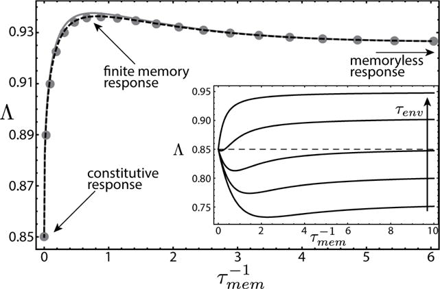
Long-term growth rate as a function of memory (both in units of b). Solid circles, numeric result obtained by averaging growth over many random realizations of environments. Error bars are smaller than symbol size. Solid (dashed) line, result of mean-field (leading order correction). Here b = 1, c = 0.3, τ_ON = 1. Environmental durations are drawn from a discrete distribution with P(0.5) = 0.7 and P(10) = 0.3. Inset: periodic model of environmental fluctuations. As environmental durations increase to satisfy cτ_env ≳ bτ_ON, the location of the optimum discontinuously transitions from infinite memory to zero memory.

Remarkably, in this model finite memory responses are optimal exclusively for random environmental fluctuations. Figure 2 shows the long-term growth rate in fluctuating environments (solid circles) overlaid with the mean-field prediction (solid line) and the leading order correction (dashed line) as functions of memory. Each gray circle is computed by numerically evolving the system of equations (7) in a random realization of environments, then averaging over many such simulations. The mean-field approximation is exact in the two opposing limits of constitutive and memoryless response, while at finite memory it slightly overestimates the long-term growth rate; it can therefore be used to distinguish if the individuals will benefit from maintaining finite phenotypic memory, or if they are more likely to evolve to one of the two limiting scenarios.

To determine how the evolution of response networks would be affected by changes in the statistics of environmental fluctuations, we calculated a phase diagram for memory optimization in the above model. Figure 3A shows a phase diagram obtained for a choice of gamma-distributed environmental durations, a two-parameter family of distributions specified by the mean ${\overline{\tau }}_{\mathit{env}}$ and variance ${\sigma }_{\mathit{env}}^2$ that are mapped in a one-to-one manner to the two axes shown. The vertical axis corresponds to the mean environmental duration, whereas the horizontal axis given by the Fano factor, ${\sigma }_{\mathit{env}}^2/{\overline{\tau }}_{\mathit{env}}$, measures the spread of the distribution of environmental durations. For tight distributions (i.e. a nearly periodic environment), the only possible optimal memory levels ${\tau }_{\mathit{mem}}^{\ast }$ correspond to constitutive $({\tau }_{\mathit{mem}}^{\ast }=\infty )$ or memoryless $({\tau }_{\mathit{mem}}^{\ast }=0)$ responses. Since the transition line is nearly flat in this regime, the optimal strategy is largely determined by the value of ${\overline{\tau }}_{\mathit{env}}$. For wide distributions, both small and large values of τ_env occur sufficiently often that finite memory can be optimal $(0<{\tau }_{\mathit{mem}}^{\ast }<\infty )$. Finite memory allows cells to avoid lags during fast fluctuations while capping the cost of memory at $c{\tau }_{\mathit{mem}}^{\ast }\ll c{\tau }_{\mathit{env}}$ during long-lasting occurrences of environment G.

FIG. 3.

(A) Evolutionary phase diagram of a gene regulatory network. The three optimization strategies cover three distinct regions in the phase space of fluctuations. Parameter values are b = 1, c = 0.3, τ_ON = 1. Variables are expressed in units of b⁻¹, hence both axes are dimensionless. Solid (dashed) lines separating optimal responses correspond to first order (continuous) phase transitions; with intersection shown at the triple point (dark circle) and the critical point (white circle). Location of the critical point is approximate. Curves of constant memory are in solid gray. The solid white curve terminating at the critical point corresponds to the critical value of memory. Arrows indicate directions along which phase transitions occur, with letters referring to panels below showing the change in fitness landscape. (B–E) First order (B, D) and continuous (C, E) phase transitions. As the statistics of the environment is varied a new maximum develops at a different value of memory and the network discontinuously or continuously crosses to the new optimum. Gray arrows indicate the direction along which phase transitions occur.

By analogy to phase diagrams of condensed matter systems, both continuous (Fig. 3A, dashed line) and first order (solid line) evolutionary phase transitions exist between these phases. First order phase transitions exhibit a jump in an order parameter $({\tau }_{\mathit{mem}}^{\ast })$ as an external parameter $({\overline{\tau }}_{\mathit{env}})$ crosses a threshold value. Two such transitions are shown in Fig. 3B, D. As we increase ${\overline{\tau }}_{\mathit{env}}$ while keeping the Fano factor fixed, the network evolves from the old optimum to a new global optimum emerging at zero memory. This type of a transition corresponds to an abrupt change in the structure of response network, such as addition or deletion of a constituent gene. At the continuous phase transitions the growth rate optimum varies across a continuous range of τ_mem (Fig. 3C, E), and biologically it could correspond to a tuning of interactions among genes in the network (see e.g. [27]).

The phase diagram also features a triple point (dark circle) where the three phases separated by discontinuous and continuous phase transitions meet [37–39] and a critical point (light circle), where a sharp boundary between memoryless and finite memory response phase becomes continuous. Constant memory curves (solid gray lines) above the critical memory curve (solid white line) end at the the critical point, while curves below the critical memory end at the boundary. The critical point in the mean-field approximation occurs when $c{\overline{\tau }}_{\mathit{env}}\approx b{\tau }_{ON}$, although small perturbations arising from noisy responses may modify cost-benefit tradeoffs resulting in small shifts in the location of transitions [34].

First order phase transitions involve coexistence of the two phases at the boundary. When growth dynamics and environmental structures become more complex, coexistence for a wider range of fluctuations becomes possible [34]. The assumptions of exponential growth and infinite nutrient availability in our simple model are not crucial for the mean-field approximation and its underlying phase structure to hold on a more general level [34]. For example, in chemostats where individuals compete for limited resources and population growth and response induction depend on nutrient concentration, the same approach is successful at predicting the outcome of competitions. Likewise, the theory can be used to determine when finite population size effects become important, and to show that these effects are expected to be negligible in typical bacterial populations. Anticipatory regulation can also be analyzed within the same framework, and seen to be beneficial when environmental fluctuations are highly predictable. These results motivate further studies of more complex population and ecological dynamics.

Due to the small number of parameters and a rich phase structure, the model described here is useful for understanding fundamental aspects of evolution, specifically principles by which regulatory networks respond optimally under a wide spectrum of fluctuation timescales. Since our model does not incorporate costs of expressing sensor proteins, sensing will always be a preferred strategy. When sensing costs are accounted for, stochastic networks that avoid sensing costs can become advantageous, and the model will exhibit a more complex phase diagram that features transitions to a stochastic switching phase [23]. Additional evolutionary phases likewise exist in the limit of a continuum of phenotypic states, as shown in several different contexts [4, 18, 30]. While the coarse-grained nature of our model omits details at the molecular level, and is not designed to quantitatively predict gene expression levels, extensions that incorporate realistic models of metabolism, such as [40], have been used to predict gene expression to very close agreement with experiments [35].

In summary, we have mathematically described evolutionary phase transitions driven by changes in the statistics of environmental fluctuations. We have formulated a theory that predicts optimal responses under fluctuating conditions, and which could be broadly applied to study diverse systems from immune responses [41, 42] and viral dynamics [43] to physiological adaptations [35], drug resistance [44–46], and cooperation [47] in phenotypically diverse cellular populations.

References

- 1.Scheffer M, Carpenter S, Foley JA, Folke C, Walker B. Nature. 2001;413:591. doi: 10.1038/35098000. [DOI] [PubMed] [Google Scholar]
- 2.Kamenev A, Meerson B, Shklovskii B. Phys Rev Lett. 2008;101 doi: 10.1103/PhysRevLett.101.268103. [DOI] [PubMed] [Google Scholar]
- 3.Mustonen V, Lässig M. Trends Genet. 2009;25:111. doi: 10.1016/j.tig.2009.01.002. [DOI] [PubMed] [Google Scholar]
- 4.Chevin LM, Lande R, Mace GM. PLoS Biology. 2010;8:e1000357. doi: 10.1371/journal.pbio.1000357. [DOI] [PMC free article] [PubMed] [Google Scholar]
- 5.Kaplan S, Bren A, Zaslaver A, Dekel E, Alon U. Mol Cell. 2008;29:786. doi: 10.1016/j.molcel.2008.01.021. [DOI] [PMC free article] [PubMed] [Google Scholar]
- 6.Sourjik V, Berg H. Proc Natl Acad Sci USA. 2002;99:123. doi: 10.1073/pnas.011589998. [DOI] [PMC free article] [PubMed] [Google Scholar]
- 7.Young JW, Locke JCW, Elowitz MB. Proc Natl Acad Sci USA. 2013;110:4140. doi: 10.1073/pnas.1213060110. [DOI] [PMC free article] [PubMed] [Google Scholar]
- 8.Tagkopoulos I, Liu YC, Tavazoie S. Science. 2008;320:1313. doi: 10.1126/science.1154456. [DOI] [PMC free article] [PubMed] [Google Scholar]
- 9.Mitchell A, Romano GH, Groisman B, Yona A, Dekel E, Kupiec M, Dahan O, Pilpel Y. Nature. 2009;460:220. doi: 10.1038/nature08112. [DOI] [PubMed] [Google Scholar]
- 10.Pattanayak GK, Lambert G, Bernat K, Rust MJ. Cell Reports. 2016;13:2362. doi: 10.1016/j.celrep.2015.11.031. [DOI] [PMC free article] [PubMed] [Google Scholar]
- 11.Balaban N, Merrin J, Chait R, Kowalik L, Leibler S. Science. 2004;305:1622. doi: 10.1126/science.1099390. [DOI] [PubMed] [Google Scholar]
- 12.Suel GM, Garcia-Ojalvo J, Liberman LM, Elowitz MB. Nature. 2006;440:545. doi: 10.1038/nature04588. [DOI] [PubMed] [Google Scholar]
- 13.Acar M, Mettetal JT, van Oudenaarden A. Nat Genet. 2008;40:471. doi: 10.1038/ng.110. [DOI] [PubMed] [Google Scholar]
- 14.Friedman N, Cai L, Xie XS. Phys Rev Lett. 2006;97:168302. doi: 10.1103/PhysRevLett.97.168302. [DOI] [PubMed] [Google Scholar]
- 15.Shahrezaei V, Swain P. Proc Natl Acad Sci USA. 2008;105:7. doi: 10.1073/pnas.0803850105. [DOI] [PMC free article] [PubMed] [Google Scholar]
- 16.Assaf M, Roberts E, Luthey-Schulten Z, Goldenfeld N. Phys Rev Lett. 2013;111:058102. doi: 10.1103/PhysRevLett.111.058102. [DOI] [PubMed] [Google Scholar]
- 17.Roberts E, Be’er S, Bohrer C, Sharma R, Assaf M. Phys Rev E. 2015;92:062717. doi: 10.1103/PhysRevE.92.062717. [DOI] [PubMed] [Google Scholar]
- 18.Haccou P, Iwasa Y. Theo Pop Biol. 1995;47:212. [Google Scholar]
- 19.Jablonka E, Oborny B, Molnar I, Kisdi E, Hofbauer J, Czaran T. Phil Trans R Soc B. 1995;350:133. doi: 10.1098/rstb.1995.0147. [DOI] [PubMed] [Google Scholar]
- 20.Lachmann M, Jablonka E. J Theor Biol. 1996;181:1. doi: 10.1006/jtbi.1996.0109. [DOI] [PubMed] [Google Scholar]
- 21.Thattai M, van Oudenaarden A. Genetics. 2004;167:523. doi: 10.1534/genetics.167.1.523. [DOI] [PMC free article] [PubMed] [Google Scholar]
- 22.Wolf DM, Vazirani VV, Arkin AP. J Theor Biol. 2005;234:227. doi: 10.1016/j.jtbi.2004.11.020. [DOI] [PubMed] [Google Scholar]
- 23.Kussell E, Leibler S. Science. 2005;309:2075. doi: 10.1126/science.1114383. [DOI] [PubMed] [Google Scholar]
- 24.Gaal B, Pitchford JW, Wood AJ. Genetics. 2010;184:1113. doi: 10.1534/genetics.109.113431. [DOI] [PMC free article] [PubMed] [Google Scholar]
- 25.Rivoire O, Leibler S. J Stat Phys. 2011;142:1124. [Google Scholar]
- 26.Filiba E, Lewin D, Brenner N. Theo Pop Biol. 2012;82:187. doi: 10.1016/j.tpb.2012.06.004. [DOI] [PubMed] [Google Scholar]
- 27.Roh K, Safaei FRP, Hespanha JP, Proulx SR. Evolution. 2013;67:1091. doi: 10.1111/evo.12012. [DOI] [PubMed] [Google Scholar]
- 28.Patra P, Klumpp S. Phys Biol. 2015;12:046004. doi: 10.1088/1478-3975/12/4/046004. [DOI] [PubMed] [Google Scholar]
- 29.Rando OJ, Verstrepen KJ. Cell. 2007;128:655. doi: 10.1016/j.cell.2007.01.023. [DOI] [PubMed] [Google Scholar]
- 30.Rivoire O, Leibler S. Proc Natl Acad Sci USA. 2014;111:E1940. doi: 10.1073/pnas.1323901111. [DOI] [PMC free article] [PubMed] [Google Scholar]
- 31.Kussell E, Leibler S, Grosberg A. Phys Rev Lett. 2006;97:068101. doi: 10.1103/PhysRevLett.97.068101. [DOI] [PubMed] [Google Scholar]
- 32.Safaei FRP, Roh K, Proulx SR, Hespanha JP. Automatica. 2014;50:2822. [Google Scholar]
- 33.Here we will restrict to a single P (τenv) that equally describes fluctuations in all environments. Generalizations where the distribution of durations depends also on the state of environment are straightforward.
- 34.See Supplementary Material [url], which includes Ref. [48].
- 35.Lambert G, Kussell E. PLoS Genet. 2014;10:e1004556. doi: 10.1371/journal.pgen.1004556. [DOI] [PMC free article] [PubMed] [Google Scholar]
- 36.Dekel E, Alon U. Nature. 2005;436:588. doi: 10.1038/nature03842. [DOI] [PubMed] [Google Scholar]
- 37.Landau LD, Lifshitz IM. Statistical physics. Pergamon Press; Oxford: 1968. Chap. 14. [Google Scholar]
- 38.Hornreich RM, Luban M, Shtrikman S. Phys Rev Lett. 1975;35:1678. [Google Scholar]
- 39.Hornreich R. J Magn Magn Mater. 1980;15:387. [Google Scholar]
- 40.Dreisigmeyer DW, Stajic J, Nemenman I, Hlavacek WS, Wall ME. IET Syst Biol. 2008;2:293. doi: 10.1049/iet-syb:20080095. [DOI] [PubMed] [Google Scholar]
- 41.Weinberger AD, Wolf YI, Lobkovsky E, Gilmore MS, Koonin EV. mBio. 2012;3:e00456–12. doi: 10.1128/mBio.00456-12. [DOI] [PMC free article] [PubMed] [Google Scholar]
- 42.Mayer A, Mora T, Rivoire O, Walczak AM. ArXiv e-prints. 2015:arXiv. 1511.08836 [q-bio.PE] [Google Scholar]
- 43.Greenbaum BD, Ghedin E. Curr Opin Microbiol. 2015;26:109. doi: 10.1016/j.mib.2015.06.015. [DOI] [PubMed] [Google Scholar]
- 44.Toprak E, Veres A, Michel JB, Chait R, Hartl DL, Kishony R. Nat Genet. 2012;44:101. doi: 10.1038/ng.1034. [DOI] [PMC free article] [PubMed] [Google Scholar]
- 45.Zhang Q, Lambert G, Liao D, Kim H, Robin K, Tung C, Pourmand N, Austin RH. Science. 2011;333:1764. doi: 10.1126/science.1208747. [DOI] [PubMed] [Google Scholar]
- 46.Wu A, Loutherback K, Lambert G, Estévez-Salmerón L, Tlsty TD, Austin RH, Sturm JC. Proc Natl Acad Sci USA. 2013;110:16103. doi: 10.1073/pnas.1314385110. [DOI] [PMC free article] [PubMed] [Google Scholar]
- 47.Tarnita CE, Washburne A, Martinez-Garcia R, Sgro AE, Levin SA. Proc Natl Acad Sci USA. 2015;112:2776. doi: 10.1073/pnas.1424242112. [DOI] [PMC free article] [PubMed] [Google Scholar]
- 48.Kussell E, Kishony R, Balaban N, Leibler S. Genetics. 2005;169:1807. doi: 10.1534/genetics.104.035352. [DOI] [PMC free article] [PubMed] [Google Scholar]