Pair-wise Clustering of Large Scale Granger Causality Index Matrices for Revealing Communities

Abstract

The analysis of large ensembles of time series is a fundamental challenge in different domains of biomedical image processing applications, specifically in the area of functional MRI data processing. An important aspect of such analysis is the ability to reconstruct community network structures based on interactive behavior between different nodes of the network which are captured in such time series. In this study, we start with a previously proposed novel approach that applies the linear Granger Causality concept to very high-dimensional time series. This approach is based on integrating dimensionality reduction into a multivariate time series model. If residuals of dimensionality reduced models can be transformed back into the original space, prediction errors in the high–dimensional space may be computed, and a large scale Granger Causality Index (lsGCI) is properly defined. The primary goal of this study was then to present an approach for recovering network structure from such lsGCI interactions through the application of pair-wise clustering. We specifically focus on a clustering approach based on topographic mapping of proximity data (TMP) for this purpose. We demonstrate our approach with a simulated network composed of five pair-wise different internal networks with varying strengths of community structure (based on the number of inter-network vertices). Our results suggest that such pair-wise clustering with TMP is capable of reconstructing the structure of the original network from lsGCI matrices that record the interactions between different nodes of the network when there is sufficient disparity between the intra- and inter-network vertices.

1. MOTIVATION/PURPOSE

To analyze large ensembles of time series is a fundamental challenge in many domains of biomedical image processing applications, ranging from microarray gene expression analysis to functional MRI data processing. A basic problem in quantifying directed information transfer is the consideration of effective connectivity in very high-dimensional systems. Currently, high-dimensional systems are transformed into a lower dimensional system, e.g. by Principal or Independent Component Analysis (PCA, ICA), and the connectivity structure of derived components is studied. Here the drawback is that a revealed interaction cannot be readily transferred back into the original high-dimensional space. Thus, directed interactions between the original network nodes are not revealed, which limits the interpretation of identified interaction patterns. Granger Causality (GC) is a suitable concept for assessing connectivity structures between time series. One popular approach uses principles of prediction [1], whereby application of a straightforward generalization to general time series models is enabled, providing an appropriate definition of prediction errors. Instead of analyzing interactions between derived components, a large scale GC (lsGC) approach preserves the interpretability of the original network nodes. The idea of that approach is the integration of a dimension reduction into a multivariate time series model, which allows computation of prediction errors in the original high-dimensional space.

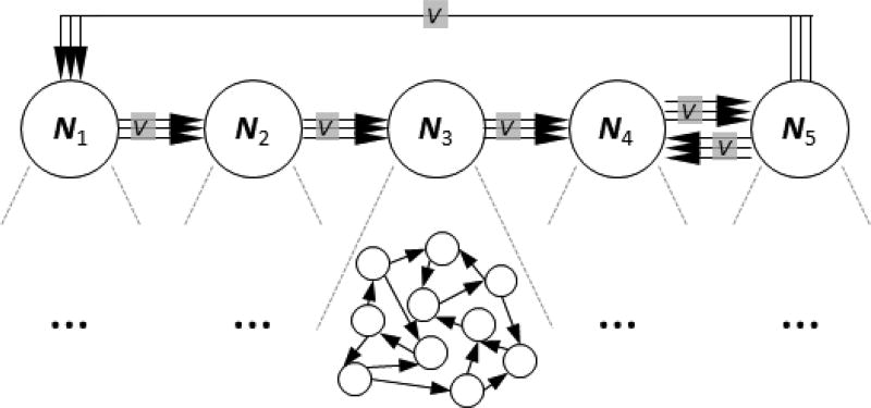
An important aspect of such analysis is the need to recover the original community network structures based on interactive behavior between different nodes of the network as captured by lsGCI. Given an lsGCI matrix that describes interactions between different nodes of a network, a pair-wise clustering approach could identify macro-networks of internal nodes thereby reconstructing the original community network structure. Such an approach could be particularly useful for biomedical image processing applications, specifically in processing functional MRI data, where such analysis with lsGCI could reveal macro-networks within the brain. In this work, we pursue a pair-wise clustering approach based on the topographic mapping of proximity (TMP) data algorithm for purposes of recovering the community structure of a simulated network with five pair-wise different internal networks, as shown in Figure 1 and discussed in the following sections.

Figure 1.

Network structure with five internal networks (communities) and a variable number V of inter-community-vertices.

2. DATA

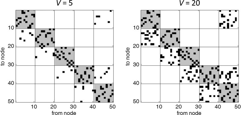
To compare the lsGCI with the conventional Granger Causality Index (GCI), we considered a time series dimensionality that can be approached by both methods. We realized 50–dimensional stationary multivariate autoregressive (MVAR) processes of order two and various time series lengths between 125 and 1000. Thereby, the entire network structure was given by five pair-wise different internal networks N₁, …, N₅ with ten nodes each (Fig. 1). The corresponding autoregressive (AR) parameters were chosen according to the AR-model of Baccala et al. [2], Fig. 4, and were scaled by factor 0.5 to ensure the stationarity of the entire process. The internal networks, or communities, N_k incorporate 20 directed vertices by setting the associated first order AR-parameter to 0.2. The in- and out-degree of each node equals two. Finally, there is a variable number V of randomly generated directed vertices from nodes of N₁ to nodes of N₂, from nodes of N₂ to nodes of N₃, etc. (see Fig. 1). Exemplarily, the corresponding adjacency matrices are shown in Fig. 2 for V = 5 and V = 20. All noise variables of the MVAR processes were i.i.d. N(0,1).

Figure 4.

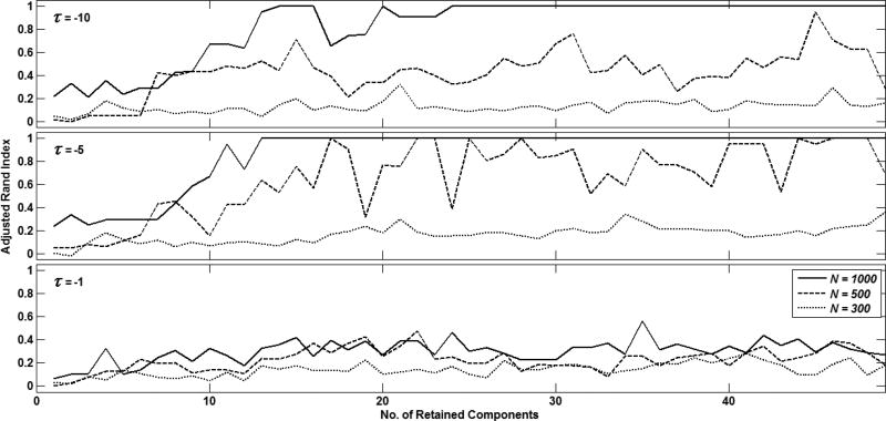
Adjusted rand index representation of clustering quality with TMP for τ = 10 (top), 5(middle) and 1 (bottom). In each sub-plot, curves are shown for N = 1000 (-), N = 500 (--) and N = 300(···).

Figure 2.

Adjacency matrices of networks with different numbers of inter-community vertices. Black squares indicate a directed vertex between two nodes. The community structure is stronger for V = 5 and comparably weak for V = 20.

3. METHODS

A D-dimensional, p^th order MVAR process is given by $\mathbf{Y}(n)={\sum }_{r=1}^p{\mathbf{A}}^r\mathbf{Y}(n-r)+\mathbf{E}(n)$, n = 1, …, N, with AR-parameters A^r ∈ ℝ^D×D and a zero mean, uncorrelated noise process E. In the case of high-dimensional data, a simple AR estimation is not possible as computational capacity rapidly meets its limits. Thus, in a first stage PCA serves as a preprocessing step for dimension reduction: X = WY, with Y = (Y(1), …, Y(N)), the principal component (PC) matrix X ∈ ℝ^D×N, and the mixing matrix W ∈ ℝ^D×D. Let X^C and W^C be the reduced PC and mixing matrices consisting of the first C rows of X and W, respectively. X^C(n) is now MVAR–modeled, and the modeled time series X̂^C(n) is afterwards transformed back into the original HD space via left multiplication of the pseudo inverse W^C+ of W^C. The residuals of the whole model are then gained by Ê = W^C+X̂^C − Y. For GCI computations, the processing of the reduced data Y^d−, where the d^th row of Y is deleted, can be performed in two different ways:

1. Multi PCA (mPCA): for every Y^d− a separate PCA is performed, i.e. ${\mathbf{X}}_m^{d-}={\mathbf{W}}_m^{d-}{\mathbf{Y}}^{d-}$, where ${\mathbf{X}}_m^{d-}$ and ${\mathbf{W}}_m^{d-}$ are calculated anew by PCA for each d. After reducing ${\mathbf{W}}_m^{d-}$ to dimension C and estimating the corresponding AR model, the modeled series ${\hat{\mathbf{X}}}_m^{d-}(n)$ can be calculated.

2. Single PCA (sPCA): only one PCA is applied before eliminating rows of Y, and modifications of the mixing matrix W are used for the dimension reduction of Y^d−, i.e. W is reduced to ${\mathbf{W}}_s^{d-}\in {ℝ}^{C\times D-1}$ by eliminating the last D − C rows and the d^th column. Now ${\mathbf{X}}_s^{d-}={\mathbf{W}}_s^{d-}{\mathbf{Y}}^{d-}$ serves for the AR parameter estimation resulting in the modeled series ${\hat{\mathbf{X}}}_s^{d-}(n)$.

The residuals amount to ${\hat{\mathbf{E}}}_{m/s}^{d-}={{\mathbf{W}}_{m/s}^{d-}}^{+}·{\hat{\mathbf{X}}}^{d-}-{\mathbf{Y}}^{d-}$. The lsGCI from d₁ to d₂ is then defined by, ${\gamma }_{d_2{d}_1}={\gamma }_{d_2\leftarrow d_1}=\text{ln}({\hat{\sum }}_{d_2}^{d_1-}/{\hat{\sum }}_{d_2})$, where Σ̂_d2 and ${\hat{\sum }}_{d_2}^{d_1-}$ are the d₂-th diagonal entries of the covariance matrices Ê and Ê^d₁−.

A detailed comparison of both approaches revealed that sPCA outperforms mPCA not only in matters of computational effort but also of correct network detection [3]. Therefore the following analyses were performed with the sPCA approach.

To further evaluate the interpretability of the original network structure from lsGCI results obtained previously, we investigated the use of a pair-wise clustering approach and evaluated its ability to accurately group internal network nodes of N₁ − N₅. Specifically, we used a soft topographic vector quantization algorithm which supported the topographic mapping of proximity (TMP) data, which can be seen as an extension of Kohonen’s self-organizing map to arbitrary distance measures. The TMP algorithm processed the data based on a dissimilarity matrix and the topographic neighborhood by a matrix of transition probabilities [4]. A detailed mathematical derivation of this algorithm and its cost function can be found in [5–6].

In this work, the dissimilarity matrix of distance measures was constructed from the lsGCI matrix that documented directed interactions between different nodes of the community network. The lsGCI matrix was then normalized to the interval [0 1] where 0 indicates no interaction between nodes while 1 indicated maximum adjacency. This was accomplished with a piece-wise continuous function f defined as

$$f({\gamma }_{\mathit{\text{ij}}})=\{\begin{array}{cc}\hfill 0,\hfill & \hfill \text{if }{\gamma }_{\mathit{\text{ij}}}\le 0\hfill \\ \hfill \frac{{\gamma }_{\mathit{\text{ij}}}}{\theta },\hfill & \hfill \text{if }0<{\gamma }_{\mathit{\text{ij}}}<\theta \hfill \\ \hfill 1,\hfill & \hfill \text{if }{\gamma }_{\mathit{\text{ij}}}\ge \theta \hfill \end{array}$$

for any two nodes i and j in the network. The lsGCI cut-off value that indicates adjacency between nodes is represented by θ here. Since θ cannot be determined without knowing the ground truth of the network, it was optimized in this work using the adjusted rand index [7–8] for maximal clustering quality. In this work, we explore using the 90^th, 95^th and 100^th percentile of the distribution of lsGCI values. The normalized lsGCI matrix was then converted to a dissimilarity matrix M as

$$m_{\mathit{\text{ij}}}=e^{-\tau ·f({\gamma }_{\mathit{\text{ij}}})}$$

where τ was an empirical constant. We note here that any monotonically declining transform could be used here, and the choice of an exponential function was empirical. In this work, we explore the effect of τ = {1, 5, 10} on the adjusted rand index achieved with the clustering algorithm. Finally the dissimilarity was symmetrized by averaging it with its transpose. Diagonal elements of the dissimilarity matrix were set to zero; while self-interaction in the nodes was not considered in our simulated network, this step was required for the clustering algorithm.

4. RESULTS

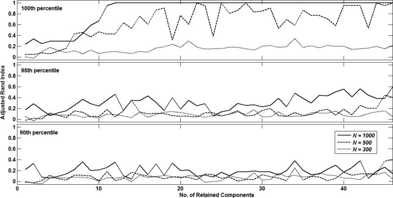
Fig. 3 shows the clustering quality achieved with different number of retained sPCA components, different time series lengths i.e. N = {1000, 500, 300} and inter-community vertices V = 1 when different values were specified for θ. As seen here, the best clustering quality was observed when θ was specified as the maximum value of the lsGCI distribution (100^th percentile). This was used for further experiments.

Figure 3.

Adjusted rand index representation of clustering quality with TMP for different values of θ, i.e. 100^th percentile (top), 95^th percentile (middle) and 90^th percentile (bottom) of lsGCIs. In each sub-plot, curves are shown for N = 1000 (-), N = 500 (--) and N = 300(···).

Fig. 4 shows the clustering quality achieved with different number of retained sPCA components, different time series lengths i.e. N = {1000, 500, 300}, and inter-community vertices V = 1 when different values are specified for τ. As seen here, the best clustering quality was observed for τ = 5, which was used for further experiments.

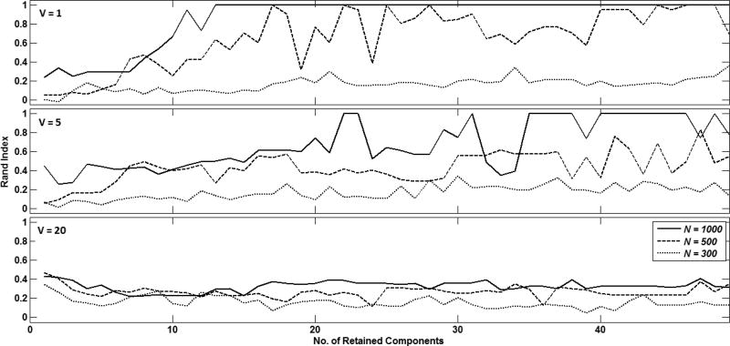
Fig. 5 shows the clustering quality achieved with different number of retained sPCA components and time series lengths N = {1000, 500, 300} for different numbers of inter-community vertices, i.e. V = {1, 5, 20}. Clustering quality was highest for N = 1000 samples when more than 10 sPCA components were retained and significant disparity was maintained between the number of intra- and inter-community vertices (top sub-plot of Fig. 5). As the number of inter-community vertices approached the number of intra-community vertices, clustering quality significantly declined (bottom sub-plot of Fig. 5). However, regardless of how many inter-community vertices were used, clustering quality was higher for larger N.

Figure 5.

Adjusted rand index representation of clustering quality with TMP when different numbers of vertices are specified between inter-community nodes N₁ − N₅ (V = 1 (top), V = 5 (middle) and V = 20 (bottom)). In each sub-plot, curves are shown for N = 1000 (-), N = 500 (--) and N = 300 (···).

5. DISCUSSION

We have previously shown PCA to be an appropriate choice for extending linear GCI to high-dimensional time series [3]. PCA reduces high-dimensional time series into lower-dimensional time series of principal components. Hereby, time series are mapped into a lower dimensional space and are subsequently modeled by an AR model. The thereby emerging residuals are transformed back into the original high-dimensional space, which offers a better interpretability of results and enables analysis of interactions between components of the original time series vs. between derived components (principal components). Alternative dimensionality reductions could also be considered if a back-transformation of the model residual from a temporary lower-dimensional space to the original high-dimensional space is allowed.

It was previously shown in [3] that an embedded dimension reduction appears to degrade the quality of the network identification when enough time series samples are available, although classical GCI was also found to yield comparable performance. For shorter time series an embedded PCA seems to result in an improvement, most likely due to smaller AR parameter matrices and reduced estimator variances. Both sPCA and mPCA approaches were investigated in [3]; sPCA was found to outperform mPCA in terms of computational effort required as well as correct network detection.

In the current study, we investigated the ability of a TMP-based clustering algorithm to cluster intra-community nodes and reconstruct the community network structure from lsGCI matrices. As seen in Fig. 5, the best results in terms of clustering quality were achieved when distinct differences in inter-community and intra-community vertices were incorporated in the network community structure. Thus, when the number of such intra- and inter-community vertices were similar, it was not possible to capture the original network structure from lsGCI matrices alone. However, regardless of how many inter-community vertices were defined, clustering quality deteriorated as the time series length was shortened. One possible reason for this deterioration could be tied to information lost during the process of converting the lsGCI matrices into dissimilarity matrices. Specifically, information related to the direction of interactions between different nodes is lost when the lsGCI is symmetrized. Such information is thus ignored by the pair-wise clustering algorithm. This will need to be studied in further detail in future studies. We are also interested in evaluating other pair-wise clustering algorithms that have been previously proposed [9–10] for purposes of recovering community network structure from lsGCI matrices. Finally, we hope to extend this approach for application to processing fMRI time series data to explore and quantify network connectivity and structure, which have been the topic of interest in several other studies [11–14].

6. CONCLUSION

This study presents a novel method to exploring effective connectivity by a Granger Causality approach with embedded dimension reduction. The applicability of our method to accurately identifying an underlying network structure has been demonstrated by quantitative analysis. We also present an application of clustering with the TMP algorithm for reconstructing network structure from lsGCI matrices. Future work will focus on applying our approach to various biomedical image processing tasks, such as microarray gene expression analysis and functional MRI data processing.

References

- 1.Granger CWJ. Investigating causal relations by econometric models and cross-spectral methods. Econometrica. 1969;37(3):424–438. [Google Scholar]
- 2.Baccala LA, Sameshima K. Partial directed coherence: a new concept in neural structure determination. Biological Cybernetics. 2001;84(6):463–474. doi: 10.1007/PL00007990. [DOI] [PubMed] [Google Scholar]
- 3.Pester B, Leistritz L, Witte H, Wismueller A. Exploring Effective Connectivity by a Granger Causality Approach with Embedded Dimension Reduction. Biomedizinische Technik/Biomedical Engineering. 2013 Sep 7; doi: 10.1515/bmt-2013-4172. [DOI] [PubMed] [Google Scholar]
- 4.Wismüller A, Lange O, Auer D, Leinsinger G. Model-Free Functional MRI Analysis for Detecting Low-Frequency Functional Connectivity in the Human Brain. Proceedings of SPIE. 2010;7624:1M1–1M6. [Google Scholar]
- 5.Graepel T, Obermayer K. A Stochastic Self-Organizing Map for Proximity Data. Neural Computation. 1999;11:139–155. doi: 10.1162/089976699300016854. [DOI] [PubMed] [Google Scholar]
- 6.Saalbach A, Twellmann T, Nattkemper TW, Wismüller A, Ontrup J, Ritter H. A Hyperbolic Topographic Mapping for Proximity Data. Artificial Intelligence and Applications. 2005;2005:106–111. [Google Scholar]
- 7.Rand WM. Objective criteria for the evaluation of clustering methods. Journal of the American Statistical Association. 1971;66(336):846–850. [Google Scholar]
- 8.Hubert L, Arabie P. Comparing partitions. Journal of Classification. 1985;2(1):193–218. [Google Scholar]
- 9.Hofmann T, Buhmann J. Multidimensional scaling and data clustering. In: Tesauro G, Touretzky D, Leen T, editors. Advances in Neural Information Processing Systems 7. Cambridge, MA: MIT Press; 1995. pp. 459–466. [Google Scholar]
- 10.Kohonen T, Somervuo P. How to make large self-organizing maps for nonvectorial data. Neural Networks. 2002;15:945–952. doi: 10.1016/s0893-6080(02)00069-2. [DOI] [PubMed] [Google Scholar]
- 11.Wismüller A, Meyer-Bäse A, Lange O, Auer D, Reiser MF, Sumners DW. Model-free functional MRI analysis based on unsupervised clustering. Journal of Biomedical Informatics. 2004;37(1):10–18. doi: 10.1016/j.jbi.2003.12.002. [DOI] [PubMed] [Google Scholar]
- 12.Meyer-Bäse A, Lange O, Wismüller A, Ritter H. Model-free functional MRI analysis using topographic independent component analysis. International journal of neural systems. 2004;14(4):217–228. doi: 10.1142/S0129065704002017. [DOI] [PubMed] [Google Scholar]
- 13.Meyer-Bäse A, Saalbach A, Lange O, Wismüller A. Unsupervised clustering of fMRI and MRI time series. Biomedical Signal Processing and Control. 2007;2(4):295–310. [Google Scholar]
- 14.Wismüller A, Dersch DR, Lipinski B, Hahn K, Auer D. Hierarchical Clustering of Functional MRI Time-Series by Deterministic Annealing. Medical Data Analysis in Lecture Notes in Computer Science. 2000;1933:49–54. [Google Scholar]