Causal mediation analysis with multiple causally non-ordered mediators

Abstract

In many health studies, researchers are interested in estimating the treatment effects on the outcome around and through an intermediate variable. Such causal mediation analyses aim to understand the mechanisms that explain the treatment effect. Although multiple mediators are often involved in real studies, most of the literature considered mediation analyses with one mediator at a time. In this article, we consider mediation analyses when there are causally non-ordered multiple mediators. Even if the mediators do not affect each other, the sum of two indirect effects through the two mediators considered separately may diverge from the joint natural indirect effect when there are additive interactions between the effects of the two mediators on the outcome. Therefore, we derive an equation for the joint natural indirect effect based on the individual mediation effects and their interactive effect, which helps us understand how the mediation effect works through the two mediators and relative contributions of the mediators and their interaction. We also discuss an extension for three mediators. The proposed method is illustrated using data from a randomized trial on the prevention of dental caries.

1 Introduction

In many health studies, researchers are interested in estimating the treatment effects on the outcome around and through an intermediate variable (called a mediator), where the corresponding effects are called direct and indirect effects, respectively, and their sum is the total effect of the treatment on the outcome of interest. Such mediation analyses aim to understand the mechanisms that explain the treatment effect. Robins and Greenland¹ originally put forward a formal study of causal mediation analysis. Following their work, Pearl² showed that a total effect can always be broken down into a natural direct and indirect effects. There is growing literature on evaluating natural direct and indirect effects.^3–11 Although a treatment often affects the outcome through multiple mediators in real studies, most of the literature considered a mediation analysis with a single mediator only.

When multiple intermediate variables are involved in a study, Daniel et al.¹² summarized existing approaches as the following three types in the setting of two mediators, M₁ and M₂ (see Figure 1(a) and (b)): (1) M₂ is the mediator of interest, and M₁ is treated as a mediator-outcome confounder affected by treatment, leading to a two-way decomposition into an effect (indirect) through M₂ and an effect (direct) not through M₂ ^13–17; (2) path-specific effects are estimated, but not in such a way that their sum equals the total effect^18,19; and (3) the multiple mediators do not causally affect one another,^20–22 that is, the arrow from M₁ to M₂ in Figure 1(a) is assumed absent (Figure 1(b)). Imai and Yamamoto²³ considered approaches for all the three conditions assuming a linear structural equation model for the outcome and mediator. Daniel et al.¹² considered the finest possible decomposition of the total effect when there are two causally ordered mediators and evaluated each path-specific effect. In addition, VanderWeele and Vansteelandt²⁴ considered the multiple mediators one at a time as joint mediators and defined the “joint” natural direct and indirect effects as an extension of the usual two-way decomposition of the total effect with regression-based approach and weighting approach.

Figure 1.

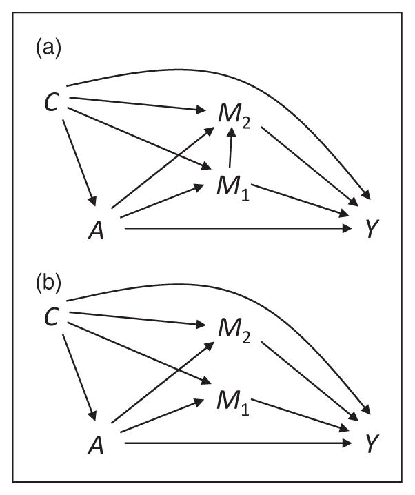
A causal diagram with treatment A, mediators M₁ and M₂, outcome Y, and confounding factors C under (a) M₁ causally affects M₂ and (b) M₁ does not causally affect M₂.

In this article, we will focus on the setting (3), that is, there are causally non-ordered multiple mediators, and provide an analytic approach to express the direct and indirect effects independent of models. Multiple mediators can be non-causally ordered when the treatment has multiple components targeting on multiple non-causally related mediators. For example, a cavity prevention plan for high-risk patients often has an antibacterial component to reduce oral bacteria as well as fluoride therapy to strength the teeth, where the two mediators oral bacteria level and fluoride level are not causally related.²⁵ With two causally non-ordered mediators involved, there are three path-specific effects from treatment (A) to outcome (Y): the direct pathway (A→Y), the indirect pathway through M₁ only (A→M₁→Y), and the indirect pathway through M₂ only (A→M₂→Y).

We can then estimate the three corresponding path-specific effects by separate analyses. Although the individual path-specific effects allow us to understand how the treatment works through individual paths alone, it may not give us the whole picture of the treatment effects involving multiple mediators. For example, consider the pathway through M₁ only. The indirect effect will be the indirect effect of the treatment through M₁, and the direct effect will thus be the effect through all other pathways including the effect through M₂. However, in a real study, researchers are often interested in how the treatment works through individual mediators (M₁ and M₂) at the same time, including their possible interaction if there is any. In such a case, a joint natural indirect effect through (M₁, M₂) will be of interest. We might then think that the sum of the two natural indirect effects for M₁ and M₂ considered separately should equal the joint natural indirect effect through (M₁, M₂). In fact, even if the two mediators do not affect each other, the sum of two indirect effects considered separately may diverge from the joint indirect effect when there are additive interactions between the effects through the two mediators on the outcome.²⁴ Therefore, in this article, we aim to provide an analytical approach to express the total effect as a function of the indirect effects through two causally non-ordered mediators (M₁, M₂) and the direct effect around (M₁, M₂) independent of models. The derived expression will help us understand how the mediation effect works through the two mediators and the relative contributions of different components and their interaction. Assumptions for identification, model-based estimation, and extension to more than two mediators will also be discussed in the article.

The remainder of this article is organized as follows: In Section 2, we briefly review the direct and indirect effects in the single mediator setting. In Section 3, we present the identification assumptions and review two existing approaches in the presence of two causally non-ordered mediators. In Section 4, we present a novel three-way decomposition of the joint natural indirect effect. In Section 5, we give the identification formula for our estimands. In Section 6, we discuss extensions to the three mediators settings, and to the vector-valued mediators. In Section 7, we apply the proposed method to data from a randomized trial evaluated the effect of a combined antibacterial and fluoride therapy on the prevention of dental caries. Finally, in Section 8, we conclude with a discussion.

2 A brief review of single mediator case

We first briefly review the direct and indirect effects for a single mediator. See Imai et al.⁹ for a more detailed explanation. Let Y denote an observed outcome for an individual, A denote a binary treatment or exposure (1: treatment or exposed, 0: control or non-exposed), C denote a set of confounding variables that may affect the treatment, mediator, and/or outcome, and M denote a single potential mediator that may be on the pathway from the treatment to the outcome (Figure 2). There may be other mediators as well but when focusing on only one mediator, the effect through other mediators would be included in the direct path from A to Y not through M.

Figure 2.

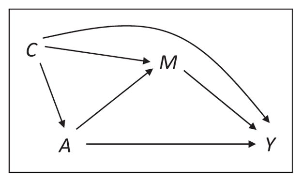
A causal diagram in a single mediator setting with treatment A, mediator M, outcome Y, and confounding factors C.

To conduct a causal mediation analysis, we use the potential outcome framework.^26,27 Let Y(a) and M(a) denote the potential outcome and potential mediator, respectively, that would be observed if, possibly contrary to the fact, A were set to a. Likewise, let Y(a,m) denote the potential outcome that would be observed if, possibly contrary to the fact, A were set to a and M were set to m. We also make assumptions referred to as the consistency and composition assumptions.⁷ The consistency assumption for (A, M) is that among the subgroup with the observed treatment A=a and the observed mediator M=m, the observed outcome Y is equal to Y(a,m). The consistency assumption for the effect of the treatment on the mediator is that among the subgroup with the observed treatment A=a, the observed mediator M is equal to M(a). The composition assumption is that Y(a)=Y(a, M(a)).

Robins and Greenland¹ and Pearl² considered the natural direct effect of treatment A on outcome Y, {Y(1, M(0))−Y(0, M(0))}. This natural direct effect compares the potential outcome under treatment and control given the mediator M at its natural level under control M(0), so is also referred as the “pure direct effect.”¹ The natural indirect effect {Y(1, M(1))−Y(1, M(0))} they considered compares the potential outcome that would be observed when the subject is treated and mediator is changed from M(0) to M(1). This natural indirect effect is also referred as the “total indirect effect.”¹ The total effect can then be decomposed into the natural direct and indirect effect as: Y(1)−Y(0)=Y(1, M(1))−Y(0, M(0))={Y(1, M(1))−Y(1, M(0))}+{Y(1, M(0))−Y(0, M(0))}. Alternatively, we can also decompose the total effect as: Y(1)−Y(0)={Y(1, M(1))−Y(0, M(1))}+{Y(0, M(1))−Y(0, M(0))}, where {Y(1, M(1))−Y(0, M(1))} is referred as the “total direct effect” and {Y(0, M(1))−Y(0, M(0))} as the “pure indirect effect.”

Because we are not able to observe all the potential outcomes for one subject in a real study, the individual level effects cannot be identified. On the other hand, under some assumptions, the population average effects can be identified. Given confounders C=c, the population average effects are conditional expectations of the individual level effects E[Y(1)−Y(0)|c], E[Y(1, M(1))−Y(1, M(0))|c], and E[Y(1, M(0))−Y(0, M(0))|c]. Various assumptions have been proposed for the identification of the population average natural direct and indirect effects. Most literature first assume no unmeasured confounding on three relationships.

• A1
  No-unmeasured confounding of the A-Y relation.

  $$Y(a,m)\coprod A\mid C\mathit{for}\mathit{all}(a,m).$$
• A2
  No-unmeasured confounding of the M-Y relation.

  $$Y(a,m)\coprod M(a)\mid A=a,C\mathit{for}\mathit{all}(a,m).$$
• A3
  No-unmeasured confounding of the A-M relation.

  $$M(a)\coprod A\mid C\mathit{for}\mathit{all}a.$$

  In addition, Pearl² made the following assumption for identification:

• A4
  A cross-world independence assumption.

  $$Y(a,m)\coprod M(a^{\ast })\mid C\mathit{for}\mathit{all}(a,a^{\ast },m).$$

If we assume that data are generated from Pearl’s nonparametric structural equation model (NPSEM),²⁸ then A4 will hold if there is no mediator-outcome confounder that is affected itself by the treatment. If a mediator-outcome confounder is affected by the treatment, then without additional assumptions, natural direct and indirect effects cannot be nonparametrically identified even under Pearl’s NPSEM irrespective of such a confounder is measured or not.¹⁸ Figure 2 shows a causal diagram that is compatible with assumptions A1–A4 under Pearl’s NPSEM.

3 Natural direct and indirect effects for two causally non-ordered mediators

3.1 Notation and assumptions

We now consider the situation that there are two causally non-ordered mediators M₁ and M₂, meaning that the causal relationship between M₁ and M₂ is absent as in Figure 1(b). In contrast, Figure 1(a) corresponds to a case where M₂ is causally affected by M₁. In this article, we will focus on the case illustrated in Figure 1(b). Let M₁(a), M₂(a), and Y(a,m₁,m₂) be obvious extensions of the potential outcomes defined in Section 2. We also assume the consistency and composition assumptions for these potential outcomes. The observed outcome Y is equal to Y(A,M₁(A),M₂(A)). We assume that the potential mediator M₂(a,m₁)=M₂(a) does not depend on the value of m₁, implying that M₂ is not causally affected by M₁.

We extend Assumptions A1–A4 to B1–B4 for two causally non-ordered mediators M₁ and M₂.

• B1
  No-unmeasured confounding of the A-Y relation.

  $$Y(a,m_1,m_2)\coprod A\mid C\mathit{for}\mathit{all}(a,m_1,m_2).$$
• B2
  No-unmeasured confounding of the (M₁, M₂)-Y relation.

  $$Y(a,m_1,m_2)\coprod \{M_1(a),M_2(a)\}\mid A=a,C\mathit{for}\mathit{all}(a,m_1,m_2).$$
• B3
  No-unmeasured confounding of the A-(M₁, M₂) relation.

  $$M_k(a)\coprod A\mid C\mathit{for}\mathit{all}(a,k).$$
• B4
  An extended cross-world independence assumption.

  $$\begin{array}{l}Y(a,m_1,m_2)\coprod \{M_1(a^{\ast }),M_2(a^{\ast \ast })\}\mid C,\\ M_1(a^{\ast })\coprod M_2(a^{\ast \ast })\mid C,\mathit{for}\mathit{all}(a,a^{\ast },a^{\ast \ast },m_1,m_2).\end{array}$$

Again, under the NPSEM, B4 will hold if there is no mediator-outcome confounder that is affected by the treatment. See Robins and Richardson²⁹ for a more detailed discussion on the NPSEM and its relation to other graphical causal models. Assumptions B1–B4 are sufficient to identify E[Y(a,M₁(a*), M₂(a**))|c] for all (a, a*, a**), as shown later in Section 5. In the remaining two subsections, we will review two existing approaches for mediation analysis in this context, and point out some counter-intuitive results.

3.2 A two-way decomposition of the total effect into the joint natural direct and indirect effects

Under the causal relationships in Figure 1(b), one may consider M₁ and M₂ as a joint mediator.²⁴ According to VanderWeele and Vansteelandt,²⁴ the natural direct and indirect effects with (M₁, M₂) as the mediator is defined by {Y(1, M₁(0), M₂(0))−Y(0, M₁(0), M₂(0))} and {Y(1, M₁(1), M₂(1)) −Y(1, M₁(0), M₂(0))}, respectively. The joint natural indirect effect here is the treatment effect mediated through M₁ or M₂, and the joint natural direct effect is the effect through neither M₁ nor M₂. Then, the total effect is decomposed into the joint natural direct and indirect effects as follows:

$$\begin{array}{l}Y(1)-Y(0)=\{Y(1,M_1(1),M_2(1))-Y(1,M_1(0),M_2(0))\}+\{Y(1,M_1(0),M_2(0))-Y(0,M_1(0),M_2(0))\}\\ =\text{total}\text{natural}\text{indirect}\text{effect}+\text{pure}\text{natural}\text{direct}\text{effect.}\end{array}$$ (1)

The definitions given in (1) are natural extensions of the decomposition of the total effect into the total indirect effect and the pure direct effect to the two mediators setting. Another similar decomposition of the total effect into the joint total direct effect and the joint pure indirect effect is given as: Y(1) −Y(0)={Y(1, M₁(1), M₂(1)) −Y(0, M₁(1), M₂(1))}+{Y(0, M₁(1), M₂(1)) −Y(0, M₁(0), M₂(0))}=total natural direct effect+pure natural indirect effect.

The differences between the “pure” and “total” direct (indirect) effects are due to the differential inclusion of the interaction between the treatment and the mediators. In a single mediator case, VanderWeele³⁰ showed that the difference {total natural direct effect–pure natural direct effect}={total natural indirect effect–pure natural indirect effect} corresponds to a “mediated interaction” between A and M, which is the product of an additive interaction of the treatment and the mediator on the outcome, {Y(1,1) −Y(1,0) −Y(0,1)+Y(0,0)}, and the effect of the treatment on the mediator, {M(1) −M(0)} (see Section 2 for the notation). This mediated interaction is arguably part of the effect that is mediated in the sense that it requires that the treatment changes the mediator.³¹ In addition, under certain assumptions, the total indirect effect, in contrast to the pure indirect effect, would give more evidence for the actual operation of mediating mechanisms.^32,33 Thus, we will focus on the decomposition (1) in the remainder of this article for illustration. However, the methods discussed in the article should be directly applied to the other decomposition.

3.3 Two three-way decompositions of the joint natural indirect effect into path-specific natural indirect effects

If our aim is to compare the relative importance of M₁ and M₂ as a mediator, then we are interested in three path-specific effects from treatment to outcome: (i) the direct effect around the two mediators (A→Y), (ii) the indirect effect through M₁ only (A→M₁→Y), and (iii) the indirect effects through M₂ only (A→M₂→Y) (Figure 1(b)). Then, the joint natural indirect effect in (1) can be further decomposed into two path-specific effects as follows:

$$Y(1,M_1(1),M_2(1))-Y(1,M_1(0),M_2(0))=\{Y(1,M_1(1),M_2(1))-Y(1,M_1(0),M_2(1))\}+\{Y(1,M_1(0),M_2(1))-Y(1,M_1(0),M_2(0))\}$$ (2)

$$=\{Y(1,M_1(1),M_2(0))-Y(1,M_1(0),M_2(0))\}+\{Y(1,M_1(1),M_2(1))-Y(1,M_1(1),M_2(0))\},$$ (3)

where the first terms in (2) and (3) are indirect effects through M₁, whereas the second terms in (2) and (3) are indirect effects through M₂. Daniel et al.¹² showed that there are six decompositions of the total effect into three path-specific effects. Of these six decompositions, Lange et al.²² focused on (2) and (3) in conjunction with (1), whereas Imai and Yamamoto²³ considered other two decompositions. In this article, we will focus on (2) and (3) because these are only two decompositions such that the sum of the indirect effects through M₁ and through M₂ is equal to the joint total natural indirect effect in (1). For the notational convenience, we use PSE₁(a)=Y(1,M₁(1), M₂(a)) −Y(1, M₁(0), M₂(a)) (a=0,1) to denote indirect effects through M₁. Likewise, we use PSE₂(a)=Y(1, M₁(a), M₂(1)) −Y(1, M₁(a), M₂(0)) (a=0,1) to denote indirect effects through M₂. Using this notation, (2)=PSE₁(1)+PSE₂(0) and (3)=PSE₁(0)+PSE₂(1).

Note that there would be no clear reason on which decomposition is preferred between (2) and (3), if we are interested in both M₁ and M₂. However, the decompositions (2) and (3) will not necessarily give the same results when PSE_k(1) ≠ PSE_k(0) (k=1,2). If the analysis results from (2) and (3) diverge in the sense that indirect effects for M₁ (M₂) are different between these two decompositions, then there is no clear guidance on which decomposition to use. Note also that using obvious notation, the total natural indirect effect through M₁ only, {Y(1, M₁(1))−Y(1, M₁(0))}, can be written as²⁴:

$$Y(1,M_1(1))-Y(1,M_1(0))=Y(1,M_1(1),M_2(1))-Y(1,M_1(0),M_2(1))={\text{PSE}}_1(1),$$ (4)

which is equal to the first term of (2). Likewise, the total natural indirect effect through M₂ only, {Y(1, M₂(1))−Y(1, M₂(0))}, can be written as:

$$Y(1,M_2(1))-Y(1,M_2(0))=Y(1,M_1(1),M_2(1))-Y(1,M_1(1),M_2(0))={\text{PSE}}_2(1),$$ (5)

which is equal to the second term of (3). From (2)–(5), we can understand that the sum of the two total natural indirect effect through M₁ (=PSE₁(1)) and M₂ (=PSE₂(1)) considered separately is not equal to the joint total natural indirect effect in general. As discussed in VanderWeele and Vansteelandt²⁴ and in Section 4, the sum of two indirect effects separately may diverge from the joint natural indirect effect when there are additive interactions between the two mediators on the outcome. Note that such interaction can arise even if the mediators do not affect each other.

4 A three-way decomposition of the joint natural indirect into path-specific natural indirect effects and an interactive effect

In Section 3, we have reviewed the existing approaches and discussed some potential problems. In this section, we present a new three-way decomposition of the joint natural indirect effect (and thus a four-way decomposition of the total effect) to resolve these problems. Here, we consider the setting of two binary mediators. Similar results are obtained for non-binary mediators (see Appendix 2). In Appendix 1, we show that the joint natural indirect effect can be further decomposed into the following three components:

$$\begin{array}{l}Y(1,M_1(1),M_2(1))-Y(1,M_1(0),M_2(0))\\ =\{Y(1,M_1(1),M_2(0))-Y(1,M_1(0),M_2(0))\}+\{Y(1,M_1(0),M_2(1))-Y(1,M_1(0),M_2(0))\}\\ +\{Y(1,M_1(1),M_2(1))-Y(1,M_1(1),M_2(0))-Y(1,M_1(0),M_2(1))+Y(1,M_1(0),M_2(0))\}\\ =\{Y(1,M_1(1),M_2(0))-Y(1,M_1(0),M_2(0))\}+\{Y(1,M_1(0),M_2(1))-Y(1,M_1(0),M_2(0))\}\\ +\{Y(1,1,1)-Y(1,1,0)-Y(1,0,1)+Y(1,0,0)\}\{M_1(1)-M_1(0)\}\{M_2(1)-M_2(0)\}.\\ ={\text{PSE}}_1(0)+{\text{PSE}}_2(0)+\text{MI}\end{array}$$ (6)

The first component in the decomposition (6) is the indirect effect through M₁ when the other mediator M₂ is set to the control level, that is, PSE₁(0). Likewise, the second component in the decomposition (6) is the indirect effect through M₂ under the other mediator M₁ is set to the control level, that is, PSE₂(0). The third component in (6) is the product of the additive interaction between M₁ andM₂ with A=1, {Y(1,1,1) −Y(1,1,0) −Y(1,0,1)+Y(1,0,0)}, the effect of the treatment onM₁, {M₁(1) −M₁(0)}, and the effect of the treatment on M₂, {M₂(1) −M₂(0)}. This interactive effect is nonzero if and only if the treatment affects both the two mediators and the additive interaction between M₁ and M₂ on Y is nonzero. Following the terminology of VanderWeele,³⁰ who considered a similar decomposition of natural direct and indirect effects in the case of a single mediator, we refer to this interactive effect as a “mediated interactive effect” or “mediated interaction” (MI) between M₁ and M₂. This three-way decomposition includes the mediated interactive effect, so that it can be explicitly evaluated in a study and also resolves the ambiguity concerning the choice between (2) and (3). By definition, it follows that MI=Y(1, M₁(1), M₂(1)) −Y(1, M₁(1), M₂(0)) −Y(1, M₁(0), M₂(1))+Y(1, M₁(0), M₂(0))=PSE₁(1) −PSE₁(0)=PSE₂(1) −PSE₂(0). Using these equalities, we obtain the following relations: PSE₁(1)=PSE₁(0)+MI and PSE₂(1)=PSE₂(0)+MI. Thus, we can understand that the difference between (2) and (3) are the differential inclusion of the mediated interaction for the indirect effect of M₁ (decomposition (2)) or for the indirect effect of M₂ (decomposition (3)). Thus, the results from (2) and (3) may diverge when there exists large additive interaction between the two mediators. Furthermore, using decomposition (6), we can understand how much of the joint natural indirect effect is explained by the interactive effect of the mediators as well as by each separate indirect effect.

Note that if the mediated interactive effect is equal to zero, then PSE₁(1)=PSE₁(0) and PSE₂(1)=PSE₂(0) hold. We then have that the joint total natural indirect effect in (6)=PSE₁(0)+PSE₂(0)=PSE₁(1)+PSE₂(1), the same as the sum of the two separate total indirect effects, (4) and (5). Conversely, if the mediated interactive effect is nonzero, then (6) diverges from the sum of (4) and (5). This fact was noted by VanderWeele and Vansteelandt²⁴ by a similar but slightly different argument.

Note that we can consider another three-way decomposition of the joint natural indirect effect in (6) using PSE₁(1) and PSE₂(1) as follows: (6)=PSE₁(1)+PSE₂(1) −MI. In this article, we focus on the decomposition in (6) for illustration. However, the methods can be directly applied to the alternative decomposition. Here, we prefer the decomposition (6) for the following two reasons. First, these two three-way decompositions give essentially the same information considering the relations PSE_k(1)=PSE_k(0)+MI (k=1,2) and it will be more natural and easier to interpret the result as the sum of PSE₁(0), PSE₂(0), and MI rather than the difference between the sum of PSE₁(1), PSE₂(2), and MI. Second, substantially, PSE_k(0) can be approximately interpreted as the effect if we had intervened only one mediator M_k while the other mediator held fixed at the control level. By contrast, PSE_k(1) can be approximately interpreted as the effect if we had intervened one mediator M_k with the other mediator held fixed at the intervention level. In our dental example in Section 7, PSE₁(0) would be interpreted as the indirect effect through M₁ (bacteria level) if we had only implemented the antibacterial treatment (although the actual intervention was the combined antibacterial and fluoride therapy). On the other hand, PSE₁(1) would be interpreted as the indirect effect through M₁ if we had implemented the antibacterial treatment for the population with the fluoride therapy uniformly implemented. Then, PSE₁(0) will be the more interesting quantity for understanding the effect through antibacterial therapy only. Similarly, we are also interested in the effect through fluoride therapy only when antibacterial therapy was not offered, that is, PSE₂(0). Therefore, equation (6) provides a natural decomposition as the sum of effect through antibacterial therapy, effect through fluoride therapy, and their interactive effect.

Given the individual level decomposition (6), we can obtain a similar decomposition in the population average effect conditional on C=c by using B4 as follows:

$$\begin{array}{l}E[Y(1,M_1(1),M_2(1))-Y(1,M_1(0),M_2(0))\mid c]\\ =E[Y(1,M_1(1),M_2(0))-Y(1,M_1(0),M_2(0))\mid c]\\ +E[Y(1,M_1(0),M_2(1))-Y(1,M_1(0),M_2(0))\mid c]\\ +E[Y(1,1,1)-Y(1,1,0)-Y(1,0,1)+Y(1,0,0)\mid c]E[M_1(1)-M_2(0)\mid c]E[M_2(1)-M_2(0)\mid c].\end{array}$$ (7)

In Appendix 2, we show the general formula which can be used for any type (i.e., non-binary) of mediators.

5 Identification

Under B1–B4, we obtain the following identification formula of E[Y(a, M₁(a*), M₂(a**))|c] for all (a, a*, a**):

$$E[Y(a,M_1(a^{\ast }),M_2(a^{\ast \ast }))\mid c]={\sum }_{m_1}{\sum }_{m_2}E[Y\mid a,m_1,m_2,c]p(m_1\mid a^{\ast },c)p(m_2\mid a^{\ast \ast },c).$$ (8)

For continuous mediators, we simply replace sums by integrals in (8). Note that (8) is a special case of Theorem 1 in Daniel et al.,¹² but we show the derivation in Appendix 3 for completeness. In addition, under B1 and B2, we have E[Y(a,m₁,m₂)|c]=E[Y|a,m₁,m₂,c], and Pr(M_k(a)=m_k |c)=p(m_k|a,c) for k=(1,2). Then, the all components in (6) as well as the joint natural direct effect can be identified from the observed data by the formulas given below:

$$\begin{array}{l}E[Y(1,M_1(0),M_2(0))-Y(0,M_1(0),M_2(0))\mid c]\\ ={\sum }_{m_1}{\sum }_{m_2}\{E[Y\mid A=1,m_1,m_2,c]-E[Y\mid A=0,m_1,m_2,c]\}p(m_1\mid A=0,c)p(m_2\mid A=0,c),\\ E[Y(1,M_1(1),M_2(0))-Y(1,M_1(0),M_2(0))\mid c]\\ ={\sum }_{m_1}{\sum }_{m_2}E[Y\mid A=1,m_1,m_2,c]\{p(m_1\mid A=1,c)-p(m_1\mid A=0,c)\}p(m_2\mid A=0,c),\\ E[Y(1,M_1(0),M_2(1))-Y(1,M_1(0),M_2(0))\mid c]\\ ={\sum }_{m_1}{\sum }_{m_2}E[Y\mid A=1,m_1,m_2,c]p(m_1\mid A=0,c)\{p(m_2\mid A=1,c)-p(m_2\mid A=0,c)\},\\ E[Y(1,1,1)-Y(1,1,0)-Y(1,0,1)+Y(1,0,0)\mid c]E[M_1(1)-M_2(0)\mid c]E[M_2(1)-M_2(0)\mid c]\\ =\{E[Y\mid A=1,M_1=1,M_2=1\mid c]-E[Y\mid A=1,M_1=1,M_2=0\mid c]-E[Y\mid A=1,M_1=0,M_2=1\mid c]\\ +E[Y\mid A=1,M_1=0,M_2=0\mid c]\}\times \{E[M_1\mid A=1,c]-E[M_1\mid A=0,c]\}\\ \times \{E[M_2\mid A=1,c]-E[M_2\mid A=0,c]\}.\end{array}$$ (9)

See Appendix 2 for the general identification formula of the mediated interactive effect for a non-binary mediator.

With counterfactual average potential outcome (8) identified, we then consider a regression approach for the estimation of observables. Suppose that Y, M₁, and M₂ are all continuous, and the following linear regression models hold for k=(1,2):

$$\begin{array}{ll}\hfill E[Y\mid a,m_1,m_2,c]& ={\theta }_0+{\theta }_{1}a+{\sum }_{k=1}^2{\theta }_2^{(k)}{m}_k+{\sum }_{k=1}^2{\theta }_3^{(k)}a{m}_k+{\theta }_4{m}_1{m}_2+{\theta }_5^{T}c,\\ \hfill E[M_k\mid a,c]& ={\beta }_0^{(k)}+{\beta }_1^{(k)}a+{\beta }_2^{(k)T}c.\end{array}$$

Then, by (8), we can show that for treatment levels a and a*, the following equalities hold:

$$\begin{array}{l}E[Y(a,M_1(a^{\ast }),M_2(a^{\ast }))-Y(a^{\ast },M_1(a^{\ast }),M_2(a^{\ast }))\mid c)]=\{{\theta }_1+{\sum }_{k=1}^2{\theta }_3^{(k)}({\beta }_0^{(k)}+{\beta }_1^{(k)}{a}^{\ast }+{\beta }_2^{(k)T}c)\}(a-a^{\ast }),\\ E[Y(a,M_1(a),M_2(a^{\ast }))-Y(a,M_1(a^{\ast }),M_2(a^{\ast }))\mid c]=\{({\theta }_2^{(1)}+{\theta }_3^{(1)}a){\beta }_1^{(1)}+{\theta }_4{\beta }_1^{(1)}({\beta }_0^{(2)}+{\beta }_1^{(2)}{a}^{\ast }+{\beta }_2^{(2)T}c)\}(a-a^{\ast }),\\ E[Y(a,M_1(a^{\ast }),M_2(a))-Y(a,M_1(a^{\ast }),M_2(a^{\ast }))\mid c]=\{({\theta }_2^{(2)}+{\theta }_3^{(2)}a){\beta }_1^{(2)}+{\theta }_4{\beta }_1^{(2)}({\beta }_0^{(1)}+{\beta }_1^{(1)}{a}^{\ast }+{\beta }_2^{(1)T}c)\}(a-a^{\ast }),\\ E[Y(a,M_1(a),M_2(a))-Y(a,M_1(a),M_2(a^{\ast }))-Y(a,M_1(a^{\ast }),M_2(a))+Y(a,M_1(a^{\ast }),M_2(a^{\ast }))\mid c]={\theta }_4{\beta }_1^{(1)}{\beta }_1^{(2)}(a-a^{\ast })(a-a^{\ast }).\end{array}$$ (10)

From (10), we can see that the mediated interactive effect is equal to zero if the additive interaction between M₁ and M₂, that is, θ₄, is equal to zero. We can also see that if θ₄ is equal to zero, then the indirect effects through M₁ and M₂ are $({\theta }_2^{(1)}+{\theta }_3^{(1)}a){\beta }_1^{(1)}(a-a^{\ast })$ and $({\theta }_2^{(2)}+{\theta }_3^{(2)}a){\beta }_1^{(2)}(a-a^{\ast })$, respectively. These are consistent with the results for the total indirect effect derived by VanderWeele and Vansteelandt⁷ in a single mediator case. Standard errors of the estimators for (10) can be obtained using the delta method.

So far we considered effects conditional on the level of the covariates C=c. To obtain marginal effect estimates, we average the expressions in (8) over the marginal distribution of C. If at least one of the mediators is continuous and a linear regression model for Y does not hold, then we cannot generally obtain analytical formulas of (8) because we have to evaluate the integral on mediators. In such a case, we can use a Monte Carlo approach according to the method described in Imai et al.⁸ to obtain marginal effect estimates. See Section 7 for the details in the application to the dental study. Standard errors and confidence intervals can be obtained based on the nonparametric bootstrap.

Another possible approach for the estimation is the inverse probability weighting (IPW).²² We can obtain an estimator of E[Y(a,M₁(a*),M₂(a**))] by taking a weighted average of the outcome Y with the following weight w_i for the individual i:

$$w_i=\frac{I(A_i=a)}{Pr(A_i=a\mid C_i=c_i)}\times \frac{Pr(M_{1i}=m_{1i}\mid A_i=a^{\ast },C_i=c_i)}{Pr(M_{1i}=m_{1i}\mid A_i=a,C_i=c_i)}\times \frac{Pr(M_{2i}=m_{2i}\mid A_i=a^{\ast \ast },C_i=c_i)}{Pr(M_{2i}=m_{2i}\mid A_i=a,C_i=c_i)},$$

where I(●) denotes the indicator function. In Appendix 4, we derive the asymptotic distribution of the IPW estimator. The regression approach above requires that the models for the outcome and mediators are correctly specified, whereas the weighting approach requires that the models for the treatment and mediators are correctly specified. The weighting approach will be more attractive if the mediation effects given in (10) is moderated by the confounders, in other words, if these effects depend on the value of c. This is because when we use the regression approach, it is difficult to specify the correct model for the outcome in the presence of the moderation by the confounders. However, the weighting approach will be unstable if some of the weights take very large values. When either the treatment or at least one of the mediators is continuous, then it is best not to use the weighting approach.

6 Extensions

6.1 Extension to the case of three mediators

Suppose that there are three causally non-ordered mediators (Figure 3(a)). Let Y(a,m₁,m₂,m₃) be a potential outcome if A, M₁, M₂, M₃ were set to a, m₁, m₂, m₃, respectively. For notational convenience, define

Figure 3.

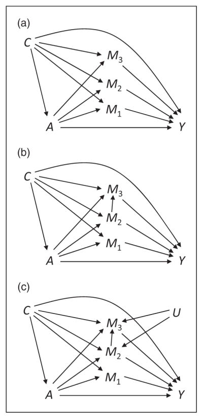
A causal diagram with treatment A, mediators M₁, M₂, and M₃, outcome Y, and confounding factors C under (a) three mediators are causally non-ordered, (b) M₂ causally affects M₃, and (c) there is unmeasured common cause U of M₂ and M₃.

$$\begin{array}{ll}\hfill {\alpha }_{12}(c)& =E[Y(1,1,1,0)-Y(1,0,1,0)-Y(1,1,0,0)+Y(1,0,0,0)\mid c],\hfill \\ \hfill {\alpha }_{13}(c)& =E[Y(1,1,0,1)-Y(1,0,0,1)-Y(1,1,0,0)+Y(1,0,0,0)\mid c],\hfill \\ \hfill {\alpha }_{23}(c)& =E[Y(1,0,1,1)-Y(1,0,0,1)-Y(1,0,1,0)+Y(1,0,0,0)\mid c],\hfill \\ \hfill {\alpha }_{123}(c)& =E[Y(1,1,1,1)-Y(1,1,1,0)-Y(1,1,0,1)-Y(1,0,1,1)+Y(1,1,0,0)+Y(1,0,1,0)+Y(1,0,0,1)-Y(1,0,0,0)\mid c],\hfill \end{array}$$

where α₁₂(c), α₁₃(c), and α₂₃(c) denote the two-way additive interaction between M₁-M₂, M₁-M₃, and M₂-M₃, respectively. α₁₂₃(c) denotes the three-way additive interaction between M₁-M₂-M₃. At the individual level, the three-way additive interaction can be rewritten as follows: {Y(1,1,1,1) − Y(1,1,0,1) − Y(1,0,1,1) + Y(1,0,0,1)} − {Y(1,1,1,0) − Y(1,1,0,0) − Y(1,0,1,0) + Y(1,0,0, 0)}. It will be nonzero if the two-way interaction between M₁ and M₂, {Y(1,1,1,m₃) − Y(1,1,0,m₃) − Y(1,0,1,m₃) + Y(1,0,0,m₃)}, is not constant across the level of m₃. Equivalently, it will be nonzero if the two-way interaction between M₁ and M₃, {Y(1,1,m₂,1) − Y(1,1,m₂,0) − Y(1,0,m₂,1) + Y(1,0,m₂,0)}, is not constant across the level of m₂, or if the two-way interaction between M₂ and M₃, {Y(1,m₁,1,1) − Y(1,m₁,1,0) − Y(1,m₁,0,1) + Y(1,m₁,0,0)}, is not constant across the level of m₁. Thus, α₁₂₃(c) describes how the two-way interactions vary across the level of the other mediator.

Suppose that the NPSEM and the mechanism shown in Figure 3(a) hold for the full data including potential outcomes. Then, following a similar argument for the derivation of (6) and (7) (see Appendices 1 and 2), we obtain the following decomposition of the joint natural indirect effect:

$$\begin{array}{l}E[Y(1,M_1(1),M_2(1),M_3(1))-Y(1,M_1(0),M_2(0),M_3(0))\mid c]\\ =E[Y(1,M_1(1),M_2(0),M_3(0))-Y(1,M_1(0),M_2(0),M_3(0))\mid c]\\ +E[Y(1,M_1(0),M_2(1),M_3(0))-Y(1,M_1(0),M_2(0),M_3(0))\mid c]\\ +E[Y(1,M_1(0),M_2(0),M_3(1))-Y(1,M_1(0),M_2(0),M_3(0))\mid c]\\ +{\sum }_{k=1}^2{\sum }_{k^{\prime }>k}^3{\delta }_k(c){\delta }_{k^{\prime }}(c){\alpha }_{k{k}^{\prime }}(c)+{\delta }_1(c){\delta }_2(c){\delta }_3(c){\alpha }_{123}(c),\end{array}$$ (11)

where δ_k(c) (k=1,2,3) denotes the effect of the treatment on M_k, E[M_k(1) − M_k(0)|c]. We refer to the last term of (11) as the mediated interactive effect between M₁, M₂, and M₃. Note that the corresponding decomposition also holds at the individual level. From (11), we see that the joint natural indirect effect is decomposed into the three indirect effect through each mediator with the other mediators at the control level, three two-way mediated interactive effects, and one three-way mediated interactive effect. Note that the three-way mediated interactive effect at the individual level, {M₁(1) − M₁(0)}{M₂(1) − M₂(0)}{M₃(1) − M₃(0)}{Y(1,1,1,1) − Y(1,1,1,0) − Y(1,1,0,1) + Y (1,0,1,1) + Y(1,1,0,0) + Y(1,0,1,0) + Y(1,0,0,1) − Y(1,0,0,0)}, is non-zero if and only if the treatment affects all three mediators, and the three-way additive interaction is non-zero.

6.2 Relaxing the identification assumptions

In previous sections, we have discussed mediation analysis when the mediators do not affect each other. In this section, we will consider the effects when two mediators lie on a causal pathway. Suppose that there are three mediators and that M₂ causally affects M₃ as in Figure 3(b). Then, the result described in Section 6.1 does not apply. Nevertheless, we consider M₂ and M₃ as a joint mediator, M₂=(M₂, M₃). Let M₂(a) be the potential value of mediator M₂ that would be observed when the subject had treatment a, and let Y(a,m₁,m₂) denote the potential outcome that would be observed when the subject had treatment a and mediators m₁ and m₂. We can define the joint natural indirect effect in a similar way as before but simply replace M₂ with the vector of two mediators M₂: {Y(1,M₁(1), M₂(1)) − Y(1, M₁(0), M₂(0))}. Then, the joint natural indirect effect can be decomposed into the indirect effect throughM₁, the indirect effect throughM₂, and the mediated interactive effect between M₁ and M₂: {Y(1, M₁(1), M₂(1)) − Y(1, M₁(0), M₂(0))}={Y(1, M₁(1), M₂(0)) − Y(1, M₁(0), M₂(0))} + {Y(1, M₁(0), M₂(1)) − Y(1, M₁(0), M₂(0))} + Σ_m1 Σ_m2 Y(1,m₁, m₂){I(M₁(1) = m₁) − I(M₁(0) = m₁)}{I(M₂(1) = m₂) − I(M₂(0) = m₂)}. Note that we can easily see that the mediated interactive effect above is non-zero only if the treatment affects M₁ and M₂, and the additive interaction between M₁ and M₂ is non-zero, that is, {Y(1,1,m₂) − Y(1,0,m₂)} is not always constant across the levels of m₂. A sufficient condition for identification of E[Y(a, M₁(a*), M₂(a**))|c] for all (a, a*, a**) is similar to B1–B4 in Section 5, but now we need to replace M₂ with M₂. These conditions hold in Figure 3(a) to 3(c).

Note that M₂ in Figure 3(b) may not be a mediator of interest but be treated as a confounder for the M₃-Y relation,¹⁶ where M₂ confounds the M₃-Y relation and, at the same time, it is affected by the treatment A. In this case, B4 is violated even if M₂ is included in the confounder set C so that the results derived in Section 4 cannot be used if M₁ and M₃ are the two mediators we are interested in. However, we can consider M₂=(M₂, M₃) and then the result described in this section can still apply.

Moreover, consider a situation that there is an unmeasured common cause U of M₂ and M₃ as in Figure 3(c). In this case, even if M₂ does not affect M₃ (i.e., there is no arrow from M₂ to M₃), the estimates of effects through the mediators M₁, M₂, and M₃ separately will be biased because when M₂ (M₃) is considered alone, U will be an unmeasured confounder for the M₂-Y (M₃-Y) relation. However, when M₂ and M₃ are considered jointly, U no longer serves as a confounder. See VanderWeele and Vansteelandt²⁴ for a related discussion on the merit of considering mediators jointly.

7 Application

In this section, we will use the methods developed in this article to understand the mediation effects in The Caries Management by Risk Assessment (CAMBRA) randomized controlled clinical trial.³⁴ CAMBRA was a randomized controlled trial, which aimed to assess whether combined antibacterial and fluoride therapy based on risk assessment has beneficial effects on preventing new caries over 24 months follow-up in adults with one to seven baseline cavitated teeth which were treated before initiating preventive therapies: the antibacterial therapy aimed to reduce oral bacteria whereas the fluoride therapy aimed to increase the fluoride level to strengthen teeth. In the study, participants in the control group (A=0) received conventional treatment per usual practices (e.g., oral hygiene instruction, periodic dental cleaning and oral examination scheduled every 6 month, radiographs scheduled every 24 month, and restorative treatment as needed), whereas participants in the intervention group (A=1) received a combined antibacterial (0.12% chlorhexidine gluconate mouth rinse) and fluoride therapy (1100 ppm sodium fluoride toothpaste, 0.05% sodium fluoride mouth rinse, and topical 1.1% NaF gel application). The primary analyses showed that the intervention group had a statistically significantly lower caries risk at follow-up and suggested a lower average caries increment compared with control over 24 months.³⁴ Our interest in this mediation analysis is whether this overall intervention effect was due mainly to bacteria reduction through antibacterial therapy, fluoride increase through fluoride therapy, or both. If observed, mediation through these mechanisms would provide further evidence for focusing future caries prevention efforts on these components.

The potential mediators of interest are two salivary oral bacteria (mutans streptococci (MS) and lactobacilli (LB)) levels and salivary fluoride level at 12 months. To make our identification assumptions more plausible, we consider MS and LB levels as a vector of mediators (M₁) and consider fluoride level as the other mediator (M₂), where M₁ and M₂ are assumed work through independent pathways. The outcome of interest (Y) was the increment from baseline in the number of decayed, missing, and filled permanent surfaces (ΔDMFS) at 24 months. ΔDMFS is a nonnegative integer count with higher values indicating worse dental outcomes. From a total of 231 participants randomized, 101 (intervention group: 51; control group: 50) patients who had completed data on ΔDMFS and relevant covariates were analyzed in this article.

Table 1 shows participants’ characteristics at baseline by intervention group. Variables that were included in the set of C were: age, sex (male/female), race (Asian/black/white/Hispanic and others), education (high school/college/graduate or professional), timing of last dental visit (less than 1 year/2 to 3 years/3 years or more), brushed 2 times or more yesterday (yes/no), used fluoride toothpaste (yes/no), fair or poor oral health (yes/no), drank alcohol in past week (yes/no), and smoked cigarette within 30 days (yes/no). Because of the positively skewed distributions, all of the three mediators were log-transformed before the mediation analysis.

Table 1.

Subjects characteristics at baseline in the CAMBRA trial.

Variables	Intervention (n = 51)	Control (n = 50)
Age (years, mean ± SD)	40.2 ± 15.1	41.3 ± 14.9
Female (n, %)	35, 68.6	31, 62.0
Race (n, %)
Asian, non-Hispanic	13, 25.5	9, 18.0
Black, non-Hispanic	7, 15.7	7, 14.0
White, non-Hispanic	8, 13.7	17, 34.0
Hispanic and others	23, 45.1	17, 34.0
Education (n, %)
High school	27, 53.0	25, 50.0
Collage	15, 29.4	15, 30.0
Graduate/professional	9, 17.7	10, 20.0
Last dental visit (n, %)
Less than 1 year	24, 47.1	19, 38.0
2 to 3 years	15, 29.4	20, 40.0
3 years or more	12, 23.5	11, 22.0
Brushed 2 or more times yesterday (n, %)	38, 74.5	39, 78.0
Used fluoride toothpaste (n, %)	37, 72.6	38, 76.0
Fair or poor oral health (n, %)	19, 37.3	21, 42.0
Drank alcohol in past week (n, %)	26, 51.0	23, 46.0
Smoked cigarette within 30 days (n, %)	7, 13.7	6, 12.0

CAMBRA: Caries Management by Risk Assessment; SD: standard deviation.

To assess whether the mediators do not affect one another (or more precisely, whether the mediators are independent of one another conditional on intervention and covariates), we first modeled p(m₂| m₁, a, c) using a linear regression model including main effects of M₁, A, and C. The p-values for MS and LB levels were 0.345 and 0.542, respectively, indicating no evidence for the violation of the assumption in the data. We therefore used the result described in Section 6.2 to estimate the direct effect, indirect effect, and mediated interaction. We modeled p(y | a, m₁, m₂, c) with a negative binomial regression and the conditional distributions of the three mediators with linear regression models assuming normally distributed errors. In addition to the main effects of all the covariates, we included interaction terms between A and M₁, A andM₂, andM₁ andM₂, in the model for the outcome. According to Imai et al.,⁸ we conducted the analyses using the following steps for the estimation of the marginal effect E[Y(a,M₁(a*), M₂(a**))]: (1) Fit the mediators and outcome models with observed data as described above. (2) Draw m₁* and m₂* from p̂(m₁|a*, c) and p̂(m₂|a**, c). (3) Draw y* from $\widehat{p}(y\mid a,{\mathbf{m}}_1^{\ast },m_2^{\ast },c)$. (4) Perform Monte Carlo replications by repeating (2) and (3) 1000 times each. (5) Compute the mean of y* over all individuals and Monte Carlo replications. 95% confidence intervals (CIs) were constructed based on the nonparametric bootstrap with 1000 resamples.

Table 2 shows various estimated direct and indirect effects of the intervention on ΔDMFS at 2 years around and through its effect on participants’ salivary bacteria and fluoride levels at 12 months. The estimated joint natural direct effect was −0.298 (95% CI: −1.894 to 1.805), and the joint natural indirect effect was −0.490 (95% CI: −1.652 to 0.172), and thus the total effect was −0.298 + (−0.490) = −0.788 (95% CI: −2.108 to 0.847). Applying the proposed three-way decomposition of the joint natural indirect effect, the indirect effect through M₁ only was −0.373 (−1.541 to 0.195), the indirect effect through M₂ only was −0.022 (95% CI: −0.366 to 0.789), and the mediated interactive effect of M₁ andM₂ was −0.095 (95% CI: −0.807 to 0.171). Thus, of the total effect, −0.298/−0.788=37.8% was attributable to the joint natural direct effect, −0.373/−0.788=47.3% was attributable to the indirect effect through M₁ only, −0.022/−0.788=2.8% was attributable to the indirect effect through M₂ only, and −0.095/−0.788=12.1% was attributable to the mediated interaction. The overall proportion mediated was 47.3 + 2.8 + 12.1=62.2%. The results indicate that the effect of the intervention (A) on ΔDMFS (Y) was mainly through its effect in decreasing salivary oral bacteria levels (M₁), although the effect is not significant due to smaller sample size for this analysis compared with primary analysis. Of the mediated effect, only a small portion of the effect was due to the effect in increasing salivary fluoride levels (M₂). However, the moderated size of the mediated interactive effect of M₁ and M₂ (more than 10%) indicates the effect of increased salivary fluoride level on ΔDMFS through its interaction with decreased oral bacterial level, which agree with the results by Cheng et al.,²⁵ where a single composite mediator “overall caries risk” was considered based on the joint values of salivary bacterial and fluoride levels with more participants included in the analysis.

Table 2.

Natural direct, indirect, and total effects of the intervention on the DMFS increment in the CAMBRA trial.

		Intervention (n = 51), Mean ± SD	Control (n = 50), Mean ± SD
Baseline	Log10 MS	4.26 ± 1.50	4.48 ± 1.30
	Log10 LB	3.72 ± 1.93	3.71 ± 1.99
	Log10 fluoride (ppm)	−1.59 ± 0.22	−1.62 ± 0.21
12 months	Log10 MS	3.25 ± 1.97	4.58 ± 1.49
	Log10 LB	2.92 ± 2.12	3.28 ± 2.00
	Log10 fluoride (ppm)	−1.38 ± 0.44	−1.54 ± 0.27
24 months	DMFS increment	3.63 ± 3.54	4.46 ± 4.16
	Joint natural direct effect (95% CI)	−0.298 (−1.894, 1.805)
	Joint natural indirect effect (95% CI)	−0.490 (−1.652, 0.172)
	M1	−0.373 (−1.541, 0.195)
	M2	−0.022 (−0.366, 0.789)
	Mediated interaction	−0.095 (−0.807, 0.171)
	Total effect	−0.788 (−2.108, 0.847)

CAMBRA: Caries Management by Risk Assessment; CI: confidence interval; DMFS: decayed missing filled permanent surfaces; LB: lactobacilli; MS: mutans streptococci; SD: standard deviation.

8 Discussion

In this article, we consider the joint natural indirect effect between two mediators as a function of the indirect effect for each mediator and the mediated interactive effect under the assumption that the mediators are not causally ordered. This relation holds even in cases when there is nonzero mediated interaction and thus a joint natural indirect effect cannot be a simple sum of the two individual natural indirect effects through the two mediator considered separately. Compared with the existing approaches described in Section 3, our proposed decomposition provides us an additional insight into the importance of the interaction among the mediators on the mediation mechanism. Such an insight may help the researchers or policymakers make a decision for a better intervention. As an example, consider a situation that there are two mediators and their mediated interactive effect is large relative to the sum of two individual mediation effects under the reference condition of the other mediator. This additional knowledge can help researchers or policymakers understand that an intervention that affects one mediator but not the other may not be the optimal option because an intervention works best when it affects both of these mediators.

We have focused on cases where the mediators do not affect each other in this article. This assumption may hold when the intervention consists of multiple independent components, which work together to improve the outcome but one component would not causally affect the other component. As in our example, in the dental study, the intervention has two components: a combined antibacterial and fluoride therapy, where the antibacterial treatment reduced oral bacteria whereas the fluoride treatment made the teeth strong. Then, the oral bacterial load and fluoride level measured at follow-up time point after the intervention would be causally non-ordered mediators between the intervention and dental outcomes, as the oral bacterial load mainly captures the effect of the antibacterial therapy, whereas the fluoride level captures the effect of the fluoride therapy.

Even if M₂ is causally affected by M₁ as Figure 1(a), our proposed decomposition of the joint natural indirect effect still holds. To be more precise, let M₂(a)=M₂(a, M₁(a)) denote the potential outcome of M₂ if A were set to a. Then, we obtain exactly the same expression as (6). However, (6) is not based on a finest possible decomposition in this case, because {Y(1, M₁(0), M₂(1)) − Y(1, M₁(0), M₂(0))}={Y(1, M₁(0), M₂(1, M₁(1))) − Y(1, M₁(0), M₂(0, M₁(0))} is the sum of the two path-specific effects A→M₂→Y, {Y(1, M₁(0), M₂(1, M₁(1))) − Y(1, M₁(0), M₂(0, M₁(1))}, and A→M₁→M₂→Y, {Y(1, M₁(0), M₂(0, M₁(1))) − Y(1, M₁(0), M₂(0, M₁(0))}. Furthermore, E[Y(a,M₁(a*),M₂(a**))|c] is not nonparametrically identified under Pearl’s NPSEM and Figure 1(a) except for the special case a*=a**.¹² Thus, we must impose additional strong assumptions for identification, or need to conduct a sensitivity analysis as described in Daniel et al.¹² Further research is needed on how to extend our method to the case of causally ordered multiple mediators.

We assume that there are no unmeasured confounders between the treatment and outcome (Assumption B1), the mediators and outcome (Assumption B2), and the treatment and mediators (Assumption B3). Although Assumptions B1 and B3 usually hold in a randomized trial, Assumption B2 does not necessarily hold even under the randomization of the treatment because the mediator cannot be randomized in a real study. In our analysis, we accounted for many potential confounders that may affect both the mediators and outcome. Even so, there may be utility in conducting sensitivity analyses that examine the effect of violations of B2. In the single mediator setting, there are many works that propose a sensitivity analysis method,^{15,17,23,35,36} including the derivation of bounds for the natural direct and indirect effects.^4,5,11,17,37 Investigation into how such methods can be adapted to this setting is another important area for future research.

Appendix 1. Derivation of (6)

We first note that the difference between the joint natural indirect effect, {Y(1, M₁(1), M₂(1)) − Y(1, M₁(0), M₂(0))}, and sum of the indirect effects for M₁, {Y(1, M₁(1), M₂(0)) − Y(1, M₁(0), M₂(0))}, and that for M₂, {Y(1, M₁(0), M₂(1)) − Y(1, M₁(0), M₂(0))}, are given by:

$$Y(1,M_1(1),M_2(1))-Y(1,M_1(1),M_2(0))-Y(1,M_1(0),M_2(1))+Y(1,M_1(0),M_2(0)).$$ (12)

For our objective, it is enough to show that (12) is equal to the third component of (6).

First, we consider to evaluate M₁(1) and M₁(0) under the fixed values of M₂(1) and M₂(0). If M₁(1) = M₁(0), then (12) = Y(1, M₁(1), M₂(1)) − Y(1, M₁(1), M₂(0)) − Y(1, M₁(1), M₂(1)) + Y(1, M₁(1), M₂(0)) = 0. If M₁(1) − M₁(0) = 1, that is, M₁(1) = 1 and M₁(0) = 0, then (12) = Y(1,1, M₂(1)) − Y(1,1, M₂(0)) − Y(1,0, M₂(1)) + Y(1,0, M₂(0)) = {Y(1,1, M₂(1)) − Y(1,1, M₂(0)) − Y(1,0, M₂(1)) + Y(1,0, M₂(0))}{M₁(1) − M₁(0)}. If M₁(1) − M₁(0) = − 1, that is, M₁(1) = 0 and M₁(0) = 1, then (12) = Y(1,0, M₂(1)) − Y(1,0, M₂(0)) − Y(1,1, M₂(1)) + Y(1,1, M₂(0)) = − {Y(1,1, M₂(1)) − Y(1,1, M₂(0)) − Y(1,0, M₂(1)) + Y(1,0, M₂(0))} = {Y(1,1, M₂(1)) − Y(1,1, M₂(0)) − Y(1,0, M₂(1)) + Y(1,0, M₂(0))}{M₁(1) − M₁(0)}. Thus, (12) can be expressed as follows:

$$\{Y(1,1,M_2(1))-Y(1,1,M_2(0))-Y(1,0,M_2(1))+Y(1,0,M_2(0))\}\{M_1(1)-M_2(0)\}.$$ (13)

Next, we consider to evaluate M₂(1) and M₂(0). If M₂(1) = M₂(0), then (13) = {Y(1,1, M₂(1)) − Y(1,1, M₂(1)) − Y(1,0, M₂(1)) + Y(1,0, M₂(1))}{M₁(1) − M₁(0)} = 0. If M₂(1) − M₂(0) = 1, that is, M₂(1) = 1 and M₂(0) = 0, then (13) = {Y(1,1,1) − Y(1,1,0) − Y(1,0,1) + Y(1,0,0)}{M₁(1) − M₁(0)} = {Y(1,1,1) − Y(1,1,0) − Y(1,0,1) + Y(1,0,0)}{M₁(1) − M₁(0)}{M₂(1) − M₂(0)}. If M₂(1) − M₂(0) = − 1, that is, M₂(1) = 0 andM₂(0) = 1, then (13) = {Y(1,1,0) − Y(1,1,1) − Y(1,0,0) + Y(1,0,1)}{M₁(1) − M₁(0)} = − {Y(1,1,1) − Y(1,1,0) − Y(1,0,1) + Y(1,0,0)}{M₁(1) − M₁(0)} = {Y(1,1,1) − Y(1,1,0) − Y(1,0,1) + Y(1,0,0)}{M₁(1) − M₁(0)}{M₂(1) − M₂(0)}. Thus, (12) is always equal to {Y(1,1,1) − Y(1,1,0) − Y(1,0,1) + Y(1,0,0)}{M₁(1) − M₁(0)}{M₂(1) − M₂(0)}, as desired.

Appendix 2. General expression of the mediated interactive effect for two mediators

We consider general types of treatments and mediators. We will compare two treatment levels, a and a*. The mediated interactive effect between M₁ and M₂ at the individual level is defined as the difference between the joint natural indirect effect, {Y(a, M₁(a), M₂(a)) − Y(a, M₁(a*), M₂(a*))}, and sum of the indirect effects for M₁, {Y(a, M₁(a), M₂(a*)) − Y(a, M₁(a*), M₂(a*))}, and that for M₂, {Y(a, M₁(a*), M₂(a)) − Y(a, M₁(a*), M₂(a*))}. It is given by,

$$\begin{array}{l}Y(a,M_1(a),M_2(a))-Y(a,M_1(a),M_2(a^{\ast }))-Y(a,M_1(a^{\ast }),M_2(a))+Y(a,M_1(a^{\ast }),M_2(a^{\ast }))\\ ={\sum }_{m_1}{\sum }_{m_2}Y(a,m_1,m_2)\{I(M_1(a)=m_1)I(M_2(a)=m_2)-I(M_1(a)=m_1)I(M_2(a^{\ast })=m_2)\\ -I(M_1(a^{\ast })=m_1)I(M_2(a)=m_2)+I(M_1(a^{\ast })=m_1)I(M_2(a^{\ast })=m_2)\}\\ ={\sum }_{m_1}{\sum }_{m_2}Y(a,m_1,m_2)[I(M_1(a)=m_1)\{I(M_2(a)=m_2)-I(M_2(a^{\ast })=m_2)\}\\ -I(M_1(a^{\ast })=m_1)\{I(M_2(a)=m_2)-I(M_2(a^{\ast })=m_2)\}]\\ ={\sum }_{m_1}{\sum }_{m_2}Y(a,m_1,m_2)\{I(M_1(a)=m_1)-I(M_1(a^{\ast })=m_1)\{I(M_2(a)=m_2)-I(M_2(a^{\ast })=m_2)\}.\end{array}$$ (14)

By taking the conditional expectation of (14) given C = c, we obtain:

$$\begin{array}{l}E[{\sum }_{m_1}{\sum }_{m_2}Y(a,m_1,m_2)\{I(M_1(a)=m_1)-I(M_1(a^{\ast })=m_1)\}\{I(M_2(a)=m_2)-I(M_2(a^{\ast })=m_2)\}\mid c]\\ ={\sum }_{m_1}{\sum }_{m_2}E[Y(a,m_1,m_2)\{I(M_1(a)=m_1)-I(M_1(a^{\ast })=m_1)\}\{I(M_2(a)=m_2)-I(M_2(a^{\ast })=m_2)\}\mid c]\\ ={\sum }_{m_1}{\sum }_{m_2}E[Y(a,m_1,m_2)\mid c]E[I(M_1(a)=m_1)-I(M_1(a^{\ast })=m_1)\mid c]\\ \times E[I(M_2(a)=m_2-I(M_2(a^{\ast })=M_2)\mid c)]\\ ={\sum }_{m_1}{\sum }_{m_2}E[Y(a,m_1,m_2)\mid c]\{Pr(M_1(a)=m_1\mid c)-Pr(M_1(a^{\ast })=m_1\mid c)\}\\ \times \{Pr(M_2(a)=m_2\mid c)-Pr(M_2(a^{\ast })=m_2\mid c)\},\end{array}$$

where the second equality follows from B4.

In summary, at the population level, we obtain the following decomposition for the total effect:

$$\begin{array}{l}E[Y(a)-Y(a^{\ast })\mid c]=E[Y(a,M_1(a^{\ast }),M_2(a^{\ast }))-Y(a^{\ast },M_1(a^{\ast }),M_2(a^{\ast }))\mid c]\\ +E[Y(a,M_1(a),M_2(a^{\ast }))-Y(a,M_1(a^{\ast }),M_2(a^{\ast }))\mid c]\\ +E[Y(a,M_1(a^{\ast }),M_2(a))-Y(a,M_1(a^{\ast }),M_2(a^{\ast }))\mid c]\\ +{\sum }_{m_1}{\sum }_{m_2}E[Y(a,m_1,m_2)\mid c]\{Pr(M_1(a)=m_1\mid c)-Pr(M_1(a^{\ast })=m_1\mid c)\}\\ \times \{Pr(M_2(a)=m_2\mid c)-Pr(M_2(a^{\ast })=m_2\mid c)\},\end{array}$$ (15)

where the first term in (15) is the joint pure natural direct effect, the second term is the indirect effect through M₁ only, and the third term is the indirect effect through M₂ only, and the fourth term is the mediated interactive effect between M₁ and M₂.

The identification formula of the first three components of (15) are given in (9) of the main text. Using the results in Section 5, the general identification formula for the fourth component is given as follows:

$$\begin{array}{l}{\sum }_{m_1}{\sum }_{m_2}E[Y(a,m_1,m_2)\mid c]\{Pr(M_1(a)=m_1\mid c)-Pr(M_1(a^{\ast })=m_1\mid c)\}\\ \times \{Pr(M_2(a)=m_2\mid c)-Pr(M_2(a^{\ast })=m_2\mid c)\}\\ ={\sum }_{m_1}{\sum }_{m_2}E[Y\mid a,m_1,m_2,c]\{p(m_1\mid a,c)-p(m_1\mid a^{\ast },c)\}\{p(m_2\mid a,c)-p(m_2\mid a^{\ast },c)\}.\end{array}$$

Appendix 3. Derivation of (8)

Under assumptions B1–B4, we have:

$$\begin{array}{l}E[Y(a,M_1(a^{\ast }),M_2(a^{\ast \ast }))\mid c]={\sum }_{m_1}{\sum }_{m_2}E[Y(a,m_1,m_2)\mid M_1(a^{\ast })=m_1,M_2(a^{\ast \ast })=M_2,c]Pr(M_1(a^{\ast })=m_1\mid c)Pr(M_2(a^{\ast \ast })=m_2\mid c)\\ ={\sum }_{m_1}{\sum }_{m_2}E[Y(a,m_1,m_2)\mid c]p(m_1\mid a^{\ast },c)p(m_2\mid a^{\ast \ast },c)\\ ={\sum }_{m_1}{\sum }_{m_2}E[Y\mid a,m_1,m_2,c]p(m_1\mid a^{\ast },c)p(m_2\mid a^{\ast \ast },c),\end{array}$$

where the first equality follows from the law of conditional expectation and B4, the second from B3 and B4, and the third from B1 and B2.

Appendix 4. Asymptotic distribution of the IPW estimator

We use large sample theory to show that the IPW estimator is asymptotically normal and derive the asymptotic variance using the standard theory of M-estimation.³⁸ This approach uses models for Pr(A = a |c) = π(a |c; γ), Pr(M₁ = m₁ |a, c) = ξ₁(m₁ |a, c; β⁽¹⁾), and Pr(M₂ = m₂ |a, c) = ξ₂(m₂ |a, c; β ⁽²⁾). We assume these probabilities are estimated by the maximum likelihood method. We first derive the influence function of the IPW estimator for E[Y(a,M₁(a*),M₂(a**))] = μ(a, a*,a**) = μ. Let β^T = (β^{(1) T}, β ^(2)T)^T and let U(μ, β, γ) = U(δ) be the estimating function corresponding to the IPW estimator:

$$U(\delta )=\frac{I(A=a)}{\pi (a\mid c;\gamma )}\times \frac{{\xi }_1(m_1\mid a^{\ast },c;{\beta }^{(1)})}{{\xi }_1(m_1\mid a,c;{\beta }^{(1)})}\times \frac{{\xi }_2(m_2\mid a^{\ast \ast },c;{\beta }^{(2)})}{{\xi }_2(m_2\mid a,c;{\beta }^{(2)})}\times (Y-\mu ).$$

Then, it follows from a Taylor series expansion that

$$\begin{array}{l}{n}^{-1/2}\sum _{i=1}^n{U}_i(\widehat{\delta })=n^{-1/2}\sum _{i=1}^n{U}_i({\delta }_0)-n^{1/2}({\widehat{\mu }}_{\mathit{IPW}}-{\mu }_0)+H_{\beta }({\delta }_0)n^{1/2}(\widehat{\beta }-{\beta }_0)+H_{\gamma }({\delta }_0)n^{1/2}(\widehat{\gamma }-{\gamma }_0)+o_p(1)\\ =n^{-1/2}\sum _{i=1}^n{U}_i({\delta }_0)-n^{1/2}({\widehat{\mu }}_{\mathit{IPW}}-{\mu }_0)+n^{-1/2}{H}_{\beta }({\delta }_0)I_{\beta }^{-1}({\beta }_0)\sum _{i=1}^n{S}_{\beta ,i}({\beta }_0)+n^{-1/2}{H}_{\gamma }({\delta }_0)I_{\gamma }^{-1}({\gamma }_0)\sum _{i=1}^n{S}_{\gamma ,i}({\gamma }_0)+o_p(1),\end{array}$$ (16)

where δ₀ = (μ₀, β₀, γ₀) are the probability limits of these estimators, H_β(δ) = E[∂U(δ)/∂β^T], H_γ(δ) = E[∂U(δ)/∂γ^T], S_.,i(.) and I.(.) are the corresponding score functions and Fisher information matrices for β and γ. Using $n^{-1/2}{\sum }_{i=1}^n{U}_i(\widehat{\delta })=0$ and (16), we obtain,

$$n^{1/2}({\widehat{\mu }}_{\mathit{IPW}}-{\mu }_0)=n^{-1/2}\sum _{i=1}^n{\psi }_i+o_p(1),$$ (17)

where ${\psi }_i=U_i({\delta }_0)+H_{\beta }({\delta }_0)I_{\beta }^{-1}({\beta }_0)S_{\beta ,i}({\beta }_0)+H_{\gamma }({\delta }_0)I_{\gamma }^{-1}({\gamma }_0)S_{\gamma ,i}({\gamma }_0)$. From the representation (17), we say that n^1/2 (μ̂_IPW − μ₀) is regular and asymptotically linear with influence function ψ_i. By replacing the unknown quantities in equation (17) with estimators, we obtain the estimated influence function ψ̂_i. It now follows from application of the central limit theorem to the representation (17), n^1/2(μ_IPW − μ₀) has an asymptotically normal distribution with mean zero and variance given by var(ψ_i). The asymptotic variance estimator is obtained by calculating the sample variance of ψ̂_i. For calculating the asymptotic variance estimators of Ê[PSE₁(0)], Ê[PSE₂(0)], and Ê[MI], we only need to calculate the sample variances of {ψ̂_i(1, 1, 0) − ψ̂_i(1, 0, 0)}, {ψ̂_i(1, 0, 1) − ψ̂_i(1, 0, 0)}, and {ψ̂_i(1, 1, 1) − ψ̂_i(1, 1, 0) − ψ̂_i(1, 0, 1) + ψ̂_i(1, 0, 0)}, respectively, where ψ̂_i(a, a^*, a^**) is the estimated influence function of the IPW estimator for μ(a, a*, a**).

References

- 1.Robins JM, Greenland S. Identifiability and exchangeability for direct and indirect effects. Epidemiology. 1992;3:143–155. doi: 10.1097/00001648-199203000-00013. [DOI] [PubMed] [Google Scholar]
- 2.Pearl J. Direct and indirect effects. Proceedings of the seventeenth conference on uncertainty in artificial intelligence; San Francisco, CA: Morgan Kaufmann; 2001. pp. 411–420. [Google Scholar]
- 3.van der Laan MJ, Petersen ML. Direct effect models. Int J Biostat. 2008;4:1–27. doi: 10.2202/1557-4679.1064. [DOI] [PubMed] [Google Scholar]
- 4.Kaufman S, Kaufman JS, MacLehose RF. Analytic bounds on causal risk differences in directed acyclic graphs involving three observed binary variables. J Stat Plan Inference. 2009;139:3473–3487. doi: 10.1016/j.jspi.2009.03.024. [DOI] [PMC free article] [PubMed] [Google Scholar]
- 5.Sjölander A. Bounds on natural effects in the presence of confounded intermediate variables. Stat Med. 2009;28:558–571. doi: 10.1002/sim.3493. [DOI] [PubMed] [Google Scholar]
- 6.VanderWeele TJ. Marginal structural models for the estimation of direct and indirect effects. Epidemiology. 2009;20:18–26. doi: 10.1097/EDE.0b013e31818f69ce. [DOI] [PubMed] [Google Scholar]
- 7.VanderWeele TJ, Vansteelandt S. Conceptual issues concerning mediation, interventions and composition. Stat Interface. 2009;2:457–468. [Google Scholar]
- 8.Imai K, Keele L, Tingley D. A general approach to causal mediation analysis. Psychol Methods. 2010;15:309–334. doi: 10.1037/a0020761. [DOI] [PubMed] [Google Scholar]
- 9.Imai K, Keele L, Yamamoto T. Identification, inference and sensitivity analysis for causal mediation effects. Stat Sci. 2010;25:51–71. [Google Scholar]
- 10.Daniels MJ, Roy JA, Kim C, et al. Bayesian inference for the causal effect of mediation. Biometrics. 2012;68:1028–1036. doi: 10.1111/j.1541-0420.2012.01781.x. [DOI] [PMC free article] [PubMed] [Google Scholar]
- 11.Chiba Y, Taguri M. Alternative monotonicity assumptions for improving bounds on natural direct effects. Int J Biostat. 2013;9:235–249. doi: 10.1515/ijb-2012-0022. [DOI] [PubMed] [Google Scholar]
- 12.Daniel RM, De Stavola BL, Cousens SN, et al. Causal mediation analysis with multiple mediators. Biometrics. 2015;71:1–14. doi: 10.1111/biom.12248. [DOI] [PMC free article] [PubMed] [Google Scholar]
- 13.Vansteelandt S, VanderWeele TJ. Natural direct and indirect effects on the exposed: effect decomposition under weaker assumptions. Biometrics. 2012;68:1019–1027. doi: 10.1111/j.1541-0420.2012.01777.x. [DOI] [PMC free article] [PubMed] [Google Scholar]
- 14.Tchetgen Tchetgen EJ, VanderWeele TJ. Identification of natural direct effects when a confounder of the mediator is directly affected by exposure. Epidemiology. 2014;25:282–291. doi: 10.1097/EDE.0000000000000054. [DOI] [PMC free article] [PubMed] [Google Scholar]
- 15.VanderWeele TJ, Chiba Y. Sensitivity analysis for direct and indirect effects in the presence of exposure-induced mediator-outcome confounders. Epidemiol Biostat Public Health. 2014;11:e9027. doi: 10.2427/9027. [DOI] [PMC free article] [PubMed] [Google Scholar]
- 16.VanderWeele TJ, Vansteelandt S, Robins JM. Effect decomposition in the presence of an exposure-induced mediator-outcome confounder. Epidemiology. 2014;25:300–306. doi: 10.1097/EDE.0000000000000034. [DOI] [PMC free article] [PubMed] [Google Scholar]
- 17.Taguri M, Chiba Y. A principal stratification approach for evaluating natural direct and indirect effects in the presence of treatment-induced intermediate confounding. Stat Med. 2015;34:131–144. doi: 10.1002/sim.6329. [DOI] [PubMed] [Google Scholar]
- 18.Avin C, Shpitser I, Pearl J. Identifiability of path-specific effects. Proceedings of the international joint conference on artificial intelligence; Edinburgh, UK: Morgan-Kaufmann; 2005. pp. 357–363. [Google Scholar]
- 19.Albert JM, Nelson S. Generalized causal mediation analysis. Biometrics. 2011;67:1028–1038. doi: 10.1111/j.1541-0420.2010.01547.x. [DOI] [PMC free article] [PubMed] [Google Scholar]
- 20.MacKinnon DP. Multivariate applications in substance use research. Mahwah, NJ: Lawrence Erlbaum Associates Publishers; 2000. Contrasts in multiple mediator models; pp. 141–160. [Google Scholar]
- 21.Preacher KJ, Hayes AF. Asymptotic and resampling strategies for assessing and comparing indirect effects in multiple mediator models. Behav Res Methods. 2008;40:879–891. doi: 10.3758/brm.40.3.879. [DOI] [PubMed] [Google Scholar]
- 22.Lange T, Rasmussen M, Thygesen LC. Assessing natural direct and indirect effects through multiple pathways. Am J Epidemiol. 2014;179:513–518. doi: 10.1093/aje/kwt270. [DOI] [PubMed] [Google Scholar]
- 23.Imai K, Yamamoto T. Identification and sensitivity analysis for multiple causal mechanisms: revisiting evidence from framing experiments. Political Anal. 2013;21:141–171. [Google Scholar]
- 24.VanderWeele TJ, Vansteelandt S. Mediation analysis with multiple mediators. Epidemiol Methods. 2013;2:95–115. doi: 10.1515/em-2012-0010. [DOI] [PMC free article] [PubMed] [Google Scholar]
- 25.Cheng J, Chaffee BW, Cheng NF, et al. Understanding treatment effect mechanisms of the CAMBRA randomized trial in reducing caries increment. J Dental Res. 2015;94:44–51. doi: 10.1177/0022034514555365. [DOI] [PMC free article] [PubMed] [Google Scholar]
- 26.Neyman J. On the application of probability theory to agricultural experiments: essay on principles, Section 9. Ann Agric Sci. 1923 Translated in Stat Sci 1990; 5: 465–472) [Google Scholar]
- 27.Rubin DB. Estimating causal effects of treatments in randomized and nonrandomized studies. J Educ Psychol. 1974;66:688–701. [Google Scholar]
- 28.Pearl J. Causality: models, reasoning, and inference. 2. New York: Cambridge University Press; 2009. [Google Scholar]
- 29.Robins JM, Richardson TS. Causality and psychopathology: finding the determinants of disorders and their cures. New York, NY: Oxford University Press; 2010. Alternative graphical causal models and the identification of direct effects; pp. 103–158. [Google Scholar]
- 30.VanderWeele TJ. A three-way decomposition of a total effect into direct, indirect, and interactive effects. Epidemiology. 2013;24:224–232. doi: 10.1097/EDE.0b013e318281a64e. [DOI] [PMC free article] [PubMed] [Google Scholar]
- 31.VanderWeele TJ. A unification of mediation and interaction: a four-way decomposition. Epidemiology. 2014;25:749–761. doi: 10.1097/EDE.0000000000000121. [DOI] [PMC free article] [PubMed] [Google Scholar]
- 32.VanderWeele TJ. Subtleties of explanatory language: what is meant by “mediation”? Eur J Epidemiol. 2011;26:343–346. doi: 10.1007/s10654-011-9588-z. [DOI] [PMC free article] [PubMed] [Google Scholar]
- 33.Suzuki E, Yamamoto E, Tsuda T. Identification of operating mediation and mechanism in the sufficient-component cause framework. Eur J Epidemiol. 2011;26:347–357. doi: 10.1007/s10654-011-9568-3. [DOI] [PubMed] [Google Scholar]
- 34.Featherstone JD, White JM, Hoover CI, et al. A randomized clinical trial of anticaries therapies targeted according to risk assessment (caries management by risk assessment) Caries Res. 2012;46:118–129. doi: 10.1159/000337241. [DOI] [PMC free article] [PubMed] [Google Scholar]
- 35.VanderWeele TJ. Bias formulas for sensitivity analysis for direct and indirect effects. Epidemiology. 2010;21:540–551. doi: 10.1097/EDE.0b013e3181df191c. [DOI] [PMC free article] [PubMed] [Google Scholar]
- 36.Tchetgen Tchetgen EJ, Shpitser I. Semiparametric theory for causal mediation analysis: efficiency bounds, multiple robustness, and sensitivity analysis. Ann Stat. 2012;40:1816–1845. doi: 10.1214/12-AOS990. [DOI] [PMC free article] [PubMed] [Google Scholar]
- 37.Tchetgen Tchetgen EJ, Phiri K. Bounds for pure direct effect. Epidemiology. 2014;25:775–776. doi: 10.1097/EDE.0000000000000154. [DOI] [PMC free article] [PubMed] [Google Scholar]
- 38.Tsiatis AA. Semiparametric theory and missing data. New York: Springer; 2006. [Google Scholar]