Data mining of magnetocardiograms for prediction of ischemic heart disease

Abstract

Ischemic Heart Disease (IHD) is a major cause of death. Early and accurate detection of IHD along with rapid diagnosis are important for reducing the mortality rate. Magnetocardiogram (MCG) is a tool for detecting electro-physiological activity of the myocardium. MCG is a fully non-contact method, which avoids the problems of skin-electrode contact in the Electrocardiogram (ECG) method. However, the interpretation of MCG recordings is time-consuming and requires analysis by an expert. Therefore, we propose the use of machine learning for identification of IHD patients. Back-propagation neural network (BPNN), the Bayesian neural network (BNN), the probabilistic neural network (PNN) and the support vector machine (SVM) were applied to develop classification models for identifying IHD patients. MCG data was acquired by sequential measurement, above the torso, of the magnetic field emitted by the myocardium using a J-T interval of 125 cases. The training and validation data of 74 cases employed 10-fold cross-validation methods to optimize support vector machine and neural network parameters. The predictive performance was assessed on the testing data of 51 cases using the following metrics: accuracy, sensitivity, and specificity and area under the receiver operating characteristic (ROC) curve. The results demonstrated that both BPNN and BNN displayed the highest and the same level of accuracy at 78.43 %. Furthermore, the decision threshold and the area under the ROC curve was -0.2774 and 0.9059, respectively, for BPNN and 0.0470 and 0.8495, respectively, for BNN. This indicated that BPNN was the best classification model, BNN was the best performing model with sensitivity of 96.65 %, and SVM employing the radial basis function kernel displayed the highest specificity of 86.36 %.

Introduction

Heart diseases are major causes of death worldwide. The World Health Organization reported that the global numbers of death caused by cardiovascular diseases are increasing every year. This is especially critical in developing counties which have increased from 14 to 25 million for 1990 to 2020, respectively. Ischemic heart disease (IHD) is considered to be a foremost disorder of the heart. It is a disease affected by long-term deficiency of oxygen and nutrient of the cardiac muscle due to inadequate supply of blood circulation. This may lead to cardiac tissue damage and cause sudden cardiac death as a consequence of heart attack.

Early diagnosis of IHD can help reduce the rate of mortality (Faculty of Science Thaksin University, 2006[10]). Electrocardiography (ECG) is traditionally applied to monitor defective electrophysiological activity of the heart. Nonetheless, in some circumstances, notification of normal ECG may be obtained albeit in the presence of angina (Tantimongcolwat et al., 2008[27]). Measurement of ECG signal by electrode-skin contact is disturbed by many type of noises (Ayari et al., 2009[2]). Therefore, magnetocardiography (MCG), a highly sensitive and contactless monitoring method of the physiological activity of the heart, has been developed. MCG essentially measures the magnetic field emission by electrophysiological activity of the heart. The magnetic field is recorded using superconducting quantum interference device (SQUID) that is without any sensor contact to the body, which is an advantage of MCG over that of ECG (Koch, 2001[17]).

MCG is more sensitive to tangential currents in the heart than ECG, and it is also sensitive to vortex current, which cannot be detected by ECG. In a normal heart, the main direction of the activation waveform is radial, from endocardium to epicardium. For these reasons, MCG may show ischemia-induced deviations from the normal direction of depolarization and repolarization with better accuracy than that of ECG (Tsukada et al., 2000[30]; Yamada and Yamaguchi, 2005[35]). MCG is affected less by conductivity variations in the body (lungs, muscles, and skin) than ECG. In addition, because MCG is a fully non-contact method, therefore problems in the skin-electrode contact as encountered in ECG are avoided (Kanzaki et al., 2003[16]; Tsukada et al., 1999[31]; Tavarozzi et al., 2002[28]).

Nowadays, medical informatics has increasingly been used to analyze large quantities of data that are stored in large databases which is made possible by the availability of powerful hardware and software along with the use of automated tools. But the interpretation of MCG recordings remains a challenge since there are no databases available from which precise rules could be deduced. The analysis of MCG data by experts is time-consuming and this is in concomitant with the shortage of experts possessing knowledge on the analysis of MCG data. Thus, methods to automate the interpretation of MCG recordings by minimizing human efforts are important for diagnosis of IHD in patients.

In this study, we used three different types of neural network and three different types of support vector machine for identification of IHD patients. The neural network classification models that are employyed is comprised of back-propagation neural network, bayesian neural network, and probabilistic neural network. The support vector machine classification models that are employed is comprised of linear, polynomial, and radial basis function kernel. All models were trained using 10-fold cross-validation technique and the optimal parameters for neural network and support vector machine were empirically determined and finally used for comparing the efficiency and accuracy of these classification models.

Material and Methods

Data acquisition and preparation

MCG data was obtained by making four sequential measurements of cardiac magnetic field at 36 locations (6 × 6 matrices) above the torso. Each of the 36 MCG signals was recorded for 90 seconds using nine sets of SQUID sensor at a sampling rate of 1000 Hz. For noise reduction purposes, the default filters setting at 0.05-100 Hz was applied and followed by an additional digital low pass filter at 20 Hz (Bick et al., 2001[4]). The MCG signals at a time window between J-point and T-peak (J-T interval) of the cardiac cycle was subdivided into 32 uniformly spaced points resulting in a set of 1,152 descriptors for all of 36 MCG signals (Froelicher et al., 2002[12]). These were assigned as inputs to build up artificial neural network models for automatic classification of IHD. The MCG datasets exploited in this study were acquired from 55 confirmed IHD cases and 70 normal individuals. Seventy-four MCG signals of both IHD and normal control groups were randomized to the training sets and the remainders were assigned as the testing set.

Overview of artificial neural network

Neural networks are the most widely used learning approach in a variety of disciplines such as business, industries and academia. A majority of the applications of neural networks has been applied for biomedical prediction and classification tasks. Mobley (Mobley et al., 2000[21]) developed neural network models for automatic detection of coronary artery stenosis using 14 risk factors for coronary artery disease. Chou (Chou et al., 2004[6]) integrated the use of artificial neural networks with multivariate adaptive regression splines approach for the classification of breast cancer. Liew compared the predictive accuracy of artificial neural networks and conventional logistic regression for the prediction of gallbladder disease in obese patients. In addition, neural network was applied for the prediction of acute coronary syndrome and was compared with multiple logistic regression (Green et al., 2006[14]).

From the above listed researches, the predictive accuracy of neural networks illustrates good performance for prediction and classification tasks. Therefore, the aim of this study was to compare the predictive accuracy of three algorithms of neural networks for prediction of ischemic heart disease from magnetocardiograms.

Overview of back-propagation neural network (BPNN)

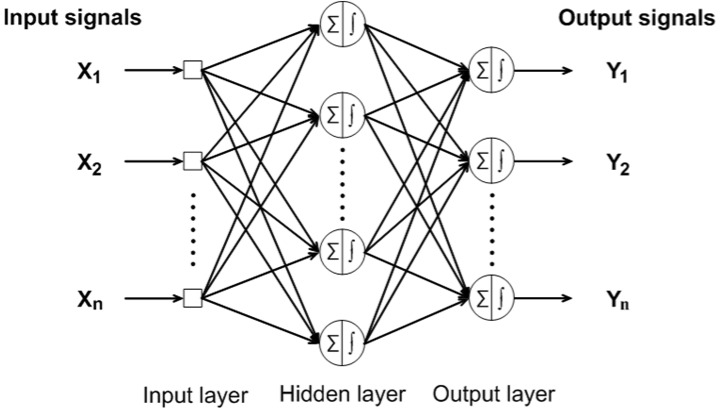
BPNN is one of the most accepted supervised feed-forward neural networks implementing the use of back-propagation learning algorithm. Input vectors and corresponding target vectors are used to train a neural network. A BPNN is composed of at least three or more layers. In this study, BPNN is consisted of three layers, where the first layer is the input layer which receives data from outside the neural network, second layer is the hidden layer which performs processing and transformation of the input data, and third layer is the output layer which sends data out of the neural network (Haykin, 1999[15]). Fig. 1(Fig. 1) shows the general BPNN architecture.

Figure 1. Architecture of a three-layer feed-forward back-propagation neural network.

The back-propagation algorithm is comprised of a forward and backward path. Forward path involves creation of a feed-forward network and weight initialization. The input vectors are propagated through the network layer by layer. Finally, a set of outputs is produced as the actual response of the network. The network weight and bias are updated in a backward path from the error, which compares the actual response with the target output. The weight updating rule can be calculated using Eq. 1:

where Δw_ji(n) is the weight update performed during the n^th iteration, α is the momentum constant, and δ_j is the error for any node (Mitchell, 1997[20]).

Overview of Bayesian neural network (BNN)

BNN uses a logistic regression model and back-propagation algorithm based on a Bayesian framework (Gao et al., 2005[13]). The class label is binary-valued y = (1,0) corresponding to normal and abnormal (IHD), respectively. A logistic regression on a Bayesian method estimates the class probability for a given input by:

The outputs from hidden and output neurons were denoted by S_j and S_k, respectively.

Hidden layer:

Output layer:

To allow the outputs to be interpreted as probabilities, the logistic regression is used to model the risk of occurrence of IHD. The logistic regression model is a S-shaped distribution which is similar condition to the estimated probabilities to lie between 0 and 1.

Let P(y = k|X) be the probability of the event y = 1 (normal case), given the input vector X. The logistic regression model as a function of network output y by:

Overview of probabilistic neural network (PNN)

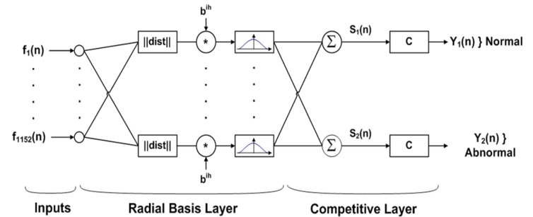
PNN is a supervised neural network (Fig. 2(Fig. 2)) that is derived from the Radial Basis Function (RBF) Network. RBF is a Gaussian function that scales the variable nonlinearly. The advantage of PNN is that it requires less training time (Comes and Kelemen, 2003[7]). In this paper, PNN has three layers: input, radial basis, and competitive layer. Radial basis layer consists of a set of RBF for evaluating the euclidean distances between input vector and row weight vectors in the weight matrix. These distances are nonlinearly scaled by Gaussian function in the radial basis layer, which is fully interconnected to a competitive layer where it passes the results to the competitive layer. Therefore, the competitive layer finds the shortest distance among them, and thus discovers the training pattern closest to the input based on their distance (Specht, 1990[26]).

Figure 2. Network structure of PNN.

Overview of support vector machine (SVM)

SVMs are a kind of supervised learning based on the statistical learning theory that was introduced by Vapnik and co-workers (Vapnik, 1998[32]; Boser et al., 1992[5]). The techniques have been further adapted by a number of other researchers (Cristianini and Shawe-Taylor, 2000[8]; Abe, 2005[1]) and they are also showing high performances in biological, chemical and medical applications (Yao et al., 2001[36]; Mehta and Lingayat, 2008[19]; Nantasenamat et al., 2008[22]).

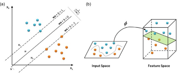
SVM is a robust technique for data classification and regression. SVM models search for a hyperplane that can linearly separate classes of objects (Fig. 3a(Fig. 3)). Let x_i ⋲ Rⁿ, (i = 1, 2, …, m) represents the vectors and y_i ⋲ {-1, 1} represents the class labels. The term f(x_i) can be represented by a linear function of the form by y_i = f(x_i)

Figure 3. Schematics of SVM depicting objects that are linearly separable (a) and non-linear mapping of input space onto the feature space (b).

where 〈w_i,x_i〉 represents the inner product of w and x, w is weight vector and b is bias. SVM approximates the set of data with linear function as follows

where

represents the feature of input variables subjected to kernel transformation while

and b are coefficients.

SVM can be applied to non-linear classification using non-linear kernel functions to map the input data onto a higher dimensional feature space in which the input data can be separated with a linear classifier (Fig. 3b(Fig. 3)). Kernel function K(x,y) represents the inner product 〈ϕ(x), ϕ(y)〉 in feature space. This study uses the following kernel functions:

Linear kernel

Polynomial kernel

where d is the degree of the polynomial (d = 0 for linear kernel).

Radial basis function kernel

where γ > 0.

Parameter optimization of neural network

The neural network architecture was selected by tuning various parameters by trial-and-error using root mean square error (RMSE) according to eq. 11.

where p_i is the predicted output, a_i is the actual output, and n is the number of com pounds in the dataset. The neural network parameters include the number of nodes in the hidden layer, the number of learning epochs, learning rate and momentum. For each of the parameter calculations, 10-fold cross-validation was performed and the average RMSE of each parameter was calculated. The lowest RMSE value of each parameter was chosen as the optimal value. In this study, to avoid overtraining 10-fold cross-validation was used for model validation (Kohavi, 1995[18]), which essentially involved the random separation of the data set into 10 fold where each fold was used once as the test set and the remaining nine-tenth was used as the training set.

The PNN training set comprising of 74 cases was trained using stratified 10-fold cross-validation. The PNN models were trained and validated for 10 times using parameters from the range of 0.1 to 5 at an interval of 0.1 (Comes and Kelemen, 2003[7]). For each case, one fold was used as the testing set while the remaining folds were used as the training set.

Confusion matrix

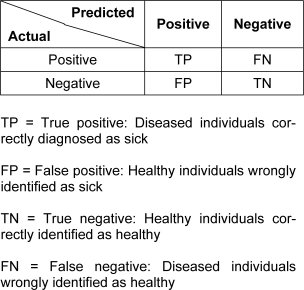
A confusion matrix contains the results about the actual and predicted classifications made by the neural network on the test set. Such information is often displayed as a two dimensional matrix. The confusion matrix is easy to understand as the correct and incorrect classification are displayed in the table (Witten and Frank, 2005[34]). The confusion matrix for a two class classifier is shown in Table 1(Tab. 1).

Table 1. Confusion matrix for a two class classifier.

Accuracy, sensitivity and specificity

Clinical research often investigates the statistical relationship between the test results and the presence of disease. In this study, we used three components that determine the performance of neural networks. Sensitivity is the probability that a test is positive (a symptom is present), given that the person has the disease.

Specificity is the probability that a test is negative (a symptom is not present), given that the person does not have the disease.

Accuracy is the proportion of correct classifications in the set of predictions.

Results

Optimization of artificial neural network

To achieve maximal performance fine-tuning of the parameters were performed. Particularly, number of nodes in the hidden layer, learning epoch size, learning rate (η) and momentum (μ) was adjusted when using BPNN and BNN while the spread parameter was optimized when using PNN.

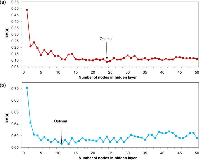
The optimal number of nodes in the hidden layer was determined by varying the number of nodes from 1 to 50 while fixing the settings for the remaining parameters. The results were plotted as a function of RMSE. The optimal value was found to be 24 and 11 for BPNN (Fig. 4a(Fig. 4)) and BNN (Fig. 4b(Fig. 4)), respectively.

Figure 4. Plot of the number of nodes in hidden layer as a function of RMSE (red square) using BPNN (a) and plot of the number of nodes in hidden layer as a function of RMSE for BNN (blue square) using BNN (b).

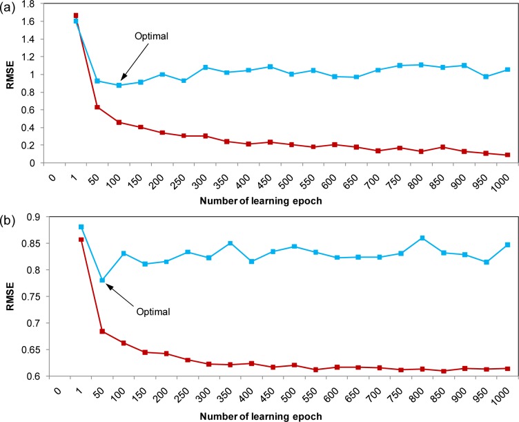
In order to avoid overtraining of the predictive model, the learning epoch size was subsequently optimized from 50 to 1000 in increments of 50 and learning was stopped once a detectable rise in RMSE for the leave-one-out cross-validated testing set was observed. By making a plot of the RMSE as a function of the learning epoch size, the best learning time was found to be 100 and 50 for BPNN (Fig. 5a(Fig. 5)) and BNN (Fig. 5b(Fig. 5)), respectively.

Figure 5. Plot of the number of learning epoch as a function of RMSE for the training set (red square) and validation set (blue square) using BPNN (a) and plot of the number of learning epoch as a function of RMSE for the training set (red square) and validation set (blue square) using BNN (b).

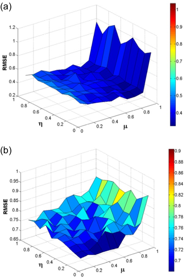
In the same manner, the optimal settings for the learning rate and momentum was determined by simultaneously varying the number of learning rate and momentum in the range of 0 to 1 and subsequently making a surface plot of RMSE against the relevant learning rates and momentums (Fig. 6(Fig. 6)). The momentum and learning rate providing a minimum global surface of error was then chosen as the optimum. It had been found that the optimal learning rate and momentum of BPNN was 0.1 and 0.7, which was nearly similar to those observed in BNN (0.1 and 0.6).

Figure 6. Surface plot of the learning rate and momentum as a function of RMSE for BPNN (a) and surface plot of the learning rate and momentum as a function of RMSE for BNN (b).

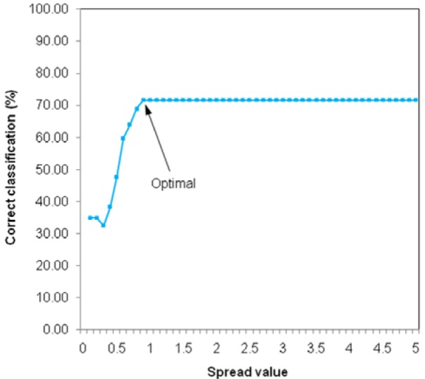
The optimization of PNN calculation was carried out in a trial-and-error manner by optimizing the spread parameter in the range of 0.1 to 5 with intervals of 0.1. The resulting prediction accuracy was then plotted as a function of the spread parameter as shown in Fig. 7(Fig. 7). It was observed that increasing the magnitude of the spread parameter resulted in an enhancement of the accuracy of prediction that was kept stable once spread parameter was in excess of 0.9. Therefore, the spread parameter of 0.9 was chosen as the optimum.

Figure 7. Plot of the spread value as a function of correct classification.

Optimization of support vector machine

For support vector machine calculations, the C parameter was optimized when using linear kernel SVM in the range of 2^-17 to 2¹⁷ at an interval of 2. Fig. 8a(Fig. 8) shows the plotting of RMSE versus C parameter. The minimum value of RMSE is optimal at C parameter of 2^-3 for linear kernel SVM.

Figure 8. Plot of the C parameter of linear kernel SVM as a function of RMSE (a), plot of the C parameter of polynomial kernel SVM as a function of RMSE (b) and surface plot of C parameter and gamma (γ) as a function of RMSE (c).

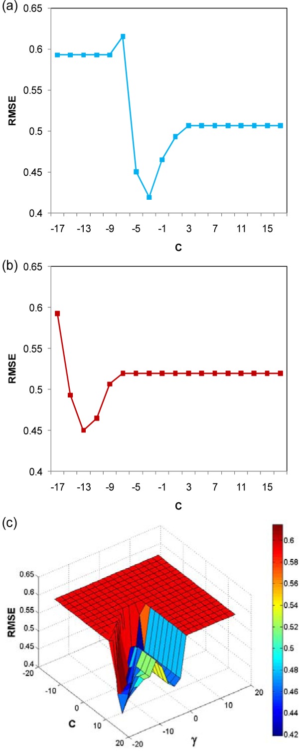
Polynomial kernel SVM has two parameters (exponent parameter and C parameter) that must be optimized. The exponent parameter was adjusted from 2 until 10 and the C parameter was adjusted from 2^-17 until 2¹⁷ by an interval of 2. We found that the optimal exponent parameter is 2² and C parameter is 2^-13 as shown in Fig. 8b(Fig. 8).

Finally, the RBF kernel SVM was optimized by adjusting the C parameter and gamma (γ) parameter by an interval of 2. The optimal value of parameter was determined by making a surface plot of RMSE as a function of C parameter and γ parameter. The optimal C parameter and γ parameter are 2¹³ and 2^-17 (Fig. 8c(Fig. 8)), respectively.

Prediction of ischemic heart disease

Machine learning models for identification of IHD were based on three learning algorithms that included BPNN, BNN and PNN. Each of the predictive models was constructed by training with 74 MCG patterns (26 IHD and 48 normal cases) under optimal parameter settings. The performance of IHD classification was then tested on 51 MCG patterns consisting of 29 IHD cases and 22 normal controls. To investigate the prediction performance and to find the optimum decision threshold, ROC curve of each model was calculated and shown in Fig. 9(Fig. 9). The decision threshold of BPNN and BNN was varied in the range of -1 to 1 and 0 to 1, respectively. The resulting prediction sensitivities were plotted as a function of one minus relevant specificities. Models giving greater area under the ROC curve provided better prediction performance than models offering the lesser area. It was observed that the area under the ROC curve given by the BPNN model was 0.9059 which was slightly higher than the BNN model which was 0.8495. The optimal decision thresholds were 0.1 and 0.5 for BPNN and BNN models, respectively. As represented in Table 2(Tab. 2), 25 out of 29 IHD cases could be correctly identified by BPNN and PNN, while only one IHD failed to be classified by BNN (see Table 2(Tab. 2)). In the classification of normal individuals, BPNN outperformed both BNN and PNN. Fifteen normal MCGs were correctly classified by BPNN, while 10 and 11 normal patterns were made by BNN and PNN.

Figure 9. ROC curve showing possible trade-offs between true positives (sensitivity) and false positives (1-specificity) for BPNN (red square) and BNN (blue square).

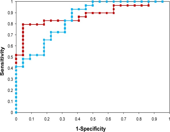
Table 2. Confusion matrix shows the prediction results of the 51 cases in the testing set.

For the SVM models, the linear kernel SVM gave the highest correctly classified accuracy of 18 out of 22 normal cases and 20 out of 29 IHD cases (see Table 2(Tab. 2)) but the highest sensitivity is obtained using polynomial kernel SVM and the highest specificity is obtained from the RBF kernel SVM (see Table 3(Tab. 3)).

Table 3. The prediction performance of classification models.

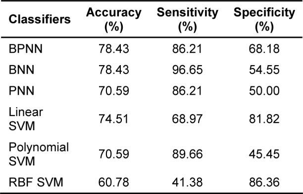
In addition, the prediction performance of these six machine learning models could be statistically demonstrated in terms of the prediction accuracy, sensitivity and specificity as shown in Table 3(Tab. 3). Comparable accuracy of prediction (78.43 %) was observed for BPNN and BNN learning models. However, BNN exhibited relatively higher sensitivity but lesser specificity of predictions than those made by BPNN.

Discussion

Machine learning plays an important role in knowledge discovery of medical data. It is widely applied for identification or classification of many diseases. For example, predicting of cancer diseases and heart diseases (Fenici et al., 2005[11]; Vibha et al., 2006[33]; Polat and Gunes, 2007[24]; Mobley et al., 2000[21]; Temurtas et al., 2009[29]). Our previous works had employed various machine algorithms in attempts to automatically distinguish between normal MCG and ischemic patterns. Under utilization of direct kernel-self organizing map (DK-SOM), direct kernel-partial least square (DK-PLS) and back propagation neural network (BPNN) on wavelet and time domains of MCG.

We employed six types of machine learning model for identification of ischemic heart disease using J-T interval of abnormal MCG pattern as inputs (Berul et al., 1994[3]; On et al., 2007[23]). On the other hand, MCG had higher sensitivity for detecting myocardial ischemia than conventional 12-lead ECG (Sato et al., 2001[25]).

As seen from previous diagnosis of IHD heart patterns with direct kernel methods, Embrechts et al. reported classification accuracy between 71 % and 83 % using direct kernel based self-organizing maps (DK-SOM), direct kernel partial least square (DK-PLS) and least-squares support vector machines (LS-SVM), which is also known as kernel ridge regression (Embrechts et al., 2003[9]). Moreover, the back-propagation neural network (BPNN) and direct kernel self-organizing map (DK-SOM) were applied for identification of IHD. The BPNN obtained 89.7 % sensitivity, 54.5 % specificity and 74.5 % accuracy, while the DK-SOM obtained higher sensitivity, specificity and accuracy than BPNN. The DK-SOM obtained 86.2 % sensitivity, 72.7 % specificity and 80.4 % accuracy (Tantimongcolwat et al., 2008[27]).

In this study, we employed various algorithms of neural network for classification task. Results of BPNN and BNN shows that both classifiers had equal performance of 78.43 % accuracy which was higher than that of the PNN classifier, which had 70.59 % classification accuracy. Sensitivity of BPNN classifier (86.21 %) was lower than that of BNN classifier (96.55 %), while specificity of BPNN classifier (68.18 %) was higher than that of BNN classifier (54.55 %). Although PNN classifier had the lowest accuracy but it also exhibited the highest specificity (73.33 %). In addition, linear kernel SVM came out to be the best performing classifier with a classification accuracy of 74.51 % but such results is still less than that of BPNN and BNN. The polynomial kernel SVM had the best sensitivity (89.66 %) but was also less than BNN. Finally, the RBF kernel had the highest specificity (86.36 %) as compared with the other classifiers.

Conclusion

This paper presents a comparative analysis of prediction model for IHD identification by using three algorithms of neural network and three kernels of support vector machine. The 125 cases were randomly separated into 74 cases for training set and 51 cases for testing set. In order to optimize the neural network structure, we used a 10-fold cross-validation on training set. The optimal parameters of neural network was determined by averaging the values from 10 runs.

Comparison of the prediction performance of IHD identification was performed using three neural network algorithms and three support vector machine kernels as applied on the 51 cases of testing sets. The result shows that BPNN and BNN gave the highest classification accuracy of 78.43 %, while RBF kernel SVM gave the lowest classification accuracy of 60.78 %. BNN presented the best sensitivity of 96.55 % and RBF kernel SVM displayed the lowest sensitivity of 41.38 %. Both polynomial kernel SVM and RBF kernel SVM presented the minimum and maximum specificity of 45.45 % and 86.36 %, respectively.

Acknowledgements

This study was supported by Mr. Karsten Sternickel, Prof. Mark J. Embrechts, and Prof. Boleslaw Szymanski for preparation of the data set used in this study and some advises for this study. Special thanks are due to Mr. Graham Pogers for partial revision of this manuscript.

References

- 1.Abe S. Support vector machines for pattern classification. New York: Springer-Verlag; 2005. [Google Scholar]
- 2.Ayari EZ, Tielert R, When N. A noise tolerant method for ECG signals feature extraction and noise reduction. Proceedings of the 3rd International Conference on Bioinformatics and Biomedical Engineering (ICBBE. 2009), 2009 June 11-13, Beijing, China.2009. [Google Scholar]
- 3.Berul CI, Sweeten TL, Dubin AM, Sham MJ, Vetter VL. Use of the rate-corrected JT interval for prediction of repolarization abnormalities in children. Am J Cardiol. 1994;74:1254–1257. doi: 10.1016/0002-9149(94)90558-4. [DOI] [PubMed] [Google Scholar]
- 4.Bick M, Sternickel K, Panaitov G, Effern A, Zhang Y, Krause HJ. SQUID gradiometry for magnetocardiography using different noise cancellation techniques. IEEE Trans Appl Supercond. 2001;11:673–676. [Google Scholar]
- 5.Boser BE, Guyon IM, Vapnik VN. A training algorithm for optimal margin classifiers. Proceedings of the 5th Annual ACM Workshop on Computational Learning Theory; Pittsburgh, USA: AMC Press; 1992. pp. 144–152. [Google Scholar]
- 6.Chou SM, Lee TS, Shao YE, Chen IF. Mining the breast cancer pattern using artificial neural networks and multivariate adaptive regression splines. Expert Syst with Appl. 2004;27:133–42. [Google Scholar]
- 7.Comes B, Kelemen A. Probabilistic neural network classification for microarraydata. Proceedings of the International Joint Conference on Neural Networks; 2003. pp. 1714–1717. [Google Scholar]
- 8.Cristianini N, Shawe-Taylor J. An introduction to support vector machines and other Kernel-based learning methods. Cambridge: Cambridge Univ. Press; 2000. [Google Scholar]
- 9.Embrechts MJ, Szymanski B, Sternickel K, Naenna T, Bragaspathi R. Use of machine learning for classification of magnetocardiograms. IEEE Int Conf Syst Man Cybernet. 2003;2:1400–1405. [Google Scholar]
- 10.Faculty of Science, Thaksin University. 2006. [19 April 2010]. Available from: www.sci.tsu.ac.th/ sciptl/radio/tape043/colesterol.doc.
- 11.Fenici R, Brisinda D, Meloni AM, Sternickel K, Fenici P. Clinical validation of machine learning for automatic analysis of multichannel magnetocardiography. In: Frangi AF, Radeva PI, Santos A, Hernandez M, editors. Functional imaging and modeling of the hear. Berlin: Springer-Verlag; 2005. pp. 143–152. [Google Scholar]
- 12.Froelicher V, Shetler K, Ashley E. Better decisions through science: Exercise testing scores. Prog Cardiovasc Dis. 2002;44:395–414. doi: 10.1053/pcad.2002.122693. [DOI] [PubMed] [Google Scholar]
- 13.Gao D, Madden M, Chambers D, Lyons G. Bayesian ANN classifier ECG arrhythmia diagnostic system: a comparison study. IEEE Int Joint Conf Neural Networks. 2005;4:2383–2388. [Google Scholar]
- 14.Green M, Bjork J, Forberg J, Ekelund U, Edenbrandt L, Ohlsson M. Comparison between neural network and multiple logistic regression to predict acute coronary syndrome in the emergency room. Artif Intell Med. 2006;38:305–318. doi: 10.1016/j.artmed.2006.07.006. [DOI] [PubMed] [Google Scholar]
- 15.Haykin S. Neural networks: a comprehensive foundation. 2nd ed. Upper Saddle River, NJ: Prentice Hall; 1999. [Google Scholar]
- 16.Kanzaki H, Nakatami S, Kandori A, Tsukada K, Miyatake K. A new screening method to diagnose coronary artery disease using multichannel magnetocardiogram and simple exercise. Basic Res Cardiol. 2003;98:124–132. doi: 10.1007/s00395-003-0392-0. [DOI] [PubMed] [Google Scholar]
- 17.Koch H. SQUID magnetocardiography: status and perspectives. IEEE Trans Appl Supercond. 2001;11:49–59. [Google Scholar]
- 18.Kohavi R. A study of study cross-validation and bootstrap for accuracy estimation and model selection. In: Mellish CS, editor. Proceedings of the 14th International Joint Conference on Artificial Intelligence, San Francisco; San Francisco, CA: Morgan Kaufman; 1995. pp. 1137–1143. [Google Scholar]
- 19.Mehta SS, Lingayat NS. Development of SVM based classification techniques for the delineation of wave components in 12-lead electrocardiogram. Biomed Signal Process. 2008;3:341–349. [Google Scholar]
- 20.Mitchell TM. Machine learning. New York: McGraw Hill; 1997. [Google Scholar]
- 21.Mobley BA, Schechter E, Moore WE, McKee PA, Eichner JE. Predictions of coronary artery stenosis by artificial neural network. Artif Intell Med. 2000;18(3):187–203. doi: 10.1016/s0933-3657(99)00040-8. [DOI] [PubMed] [Google Scholar]
- 22.Nantasenamat C, Isarankura-Na-Ayudhya C, Naenna T. Prediction of bond dissociation enthalpy of antioxidant phenols by support vector machine. J Mol Graph Model. 2008;27:188–196. doi: 10.1016/j.jmgm.2008.04.005. [DOI] [PubMed] [Google Scholar]
- 23.On K, Watanabe S, Yamada S, Takeyasu N, Nakagawa Y, Nishina H, Morimoto T, Aihara H, Kimura T, Sato Y, Tsukada K, Kandori A, Miyashita T, Ogata K, Suzuki D, Yamaguchi I, Aonuma K. Integral value of JT interval in magnetocardiography is sensitive to coronary stenosis and improves soon after coronary revascularization. Circ J. 2007;71:1586–1592. doi: 10.1253/circj.71.1586. [DOI] [PubMed] [Google Scholar]
- 24.Polat K, Gunes S. Breast cancer diagnosis using least square support vector machine. Digit Signal Process. 2007;17:694–701. [Google Scholar]
- 25.Sato M, Terada Y, Mitsui T, Miyashita T, Kandori A, Tsukada K. Detection of myocardial ischemia by magnetocardiogram using 64-channel SQUID system. In: Nenonen J, Imoniemi RJ, Katila T, editors. Proceedings of the 12th International Conference on Biomagnetism; Espoo: Helsinki University Technology; 2001. pp. 523–526. [Google Scholar]
- 26.Specht DF. Probabilistic neural networks. Neural Networks. 1990;3:109–118. doi: 10.1109/72.80210. [DOI] [PubMed] [Google Scholar]
- 27.Tantimongcolwat T, Naenna T, Isarankura-Na-Ayudhya C, Embrechts MJ, Prachayasittikul V. Identification of ischemic heart disease via machine learning analysis on magnetocardiograms. Comput Biol Med. 2008;38:817–825. doi: 10.1016/j.compbiomed.2008.04.009. [DOI] [PubMed] [Google Scholar]
- 28.Tavarozzi I, Comani S, Gratta CD, Romani GL, Luzio SD, Brisinda D, et al. Magnetocardiography: current status and perspectives. Part I: Physical principles and instrumentation. Ital Heart J. 2002;3(2):75–85. [PubMed] [Google Scholar]
- 29.Temurtas H, Yumusak N, Temurtas F. A comparative study on diabetes disease diagnosis using neural networks. Expert Syst Appl. 2009;36:8610–8615. [Google Scholar]
- 30.Tsukada K, Miyashita T, Kandori A, Yamada S, Sato M, Terada Y, et al. Magnetocardiographic mapping characteristic for diagnosis of ischemic heart disease. Comput Cardiol. 2000;27:505–508. [Google Scholar]
- 31.Tsukada K, Sasabuchi H, Mitsui T. Measuring technology for cardiac magneto-field using ultra-sensitive magnetic sensor for high speed and noninvasive cardiac examination. Hitachi Rev. 1999;48:116–119. [Google Scholar]
- 32.Vapnik VN. Statistical learning theory. New York: Wiley; 1998. [Google Scholar]
- 33.Vibha L, Harshavardhan GM, Pranaw K, Deepa Shenoy P, Venugopal KR, Patnaik LM. Classification of mammograms using decision trees. Proceedings of the 10th International Database Engineering and Applications Symposium, 2006, Dec 11-13. Delhi, India.2006. [Google Scholar]
- 34.Witten IH, Frank E. Data mining: practical machine learning tools and techniques. 2nd ed. San Francisco, CA: Morgan Kaufman; 2005. [Google Scholar]
- 35.Yamada S, Yamaguchi I. Magnetocardiograms in clinical medicine: Unique information on cardiac ischemia, arrhythmias, and fetal diagnosis. Intern Med. 2005;44:1–19. doi: 10.2169/internalmedicine.44.1. [DOI] [PubMed] [Google Scholar]
- 36.Yao Y, Frasconi P, Pontil M. Fingerprint classification with combinations of support vector machine. 3rd International Conference of Audio and Video-Based Person Authentication, 2001, June, Halmstad, Sweden; 2001. pp. 253–259. [Google Scholar]