The warmer the ocean surface, the shallower the mixed layer. How much of this is true?

Abstract

Ocean surface warming is commonly associated with a more stratified, less productive, and less oxygenated ocean. Such an assertion is mainly based on consistent projections of increased near‐surface stratification and shallower mixed layers under global warming scenarios. However, while the observed sea surface temperature (SST) is rising at midlatitudes, the concurrent ocean record shows that stratification is not unequivocally increasing nor is MLD shoaling. We find that while SST increases at three study areas at midlatitudes, stratification both increases and decreases, and MLD deepens with enhanced deepening of winter MLDs at rates over $10\hspace{0.17em}\mathrm{m} \hspace{0.17em}{\text{decade}}^{-1}$. These results rely on the estimation of several MLD and stratification indexes of different complexity on hydrographic profiles from long‐term hydrographic time‐series, ocean reanalysis, and Argo floats. Combining this information with estimated MLDs from buoyancy fluxes and the enhanced deepening/attenuation of the winter MLD trends due to changes in the Ekman pumping, MLD variability involves a subtle interplay between circulation and atmospheric forcing at midlatitudes. Besides, it is highlighted that the density difference between the surface and 200 m, the most widely used stratification index, should not be expected to reliably inform about changes in the vertical extent of mixing.

Key Points

• Ocean observations show that surface warming is not definitively linked to a more stratified and less mixed ocean

• Subtle interplay between changes in circulation and atmospheric forcing contribute to find warmer and deeper MLDs

• How our findings reconcile with the observation of a less productive and oxygenated ocean is discussed

1. Introduction

As greenhouse gases increase the Earth radiative imbalance, the oceans sequester up to 93% of the extra heat in the climate system [Alexander et al., 2013], and as a result, the ocean is warming [Balmaseda et al., 2013a, 2013b; Roemmich et al., 2015]. However, some oceanic regions absorb more heat than others, and ocean warming does not occur homogeneously in space (Figure 1) and gradually from the surface to the bottom as one might expect from a regular removal of atmospheric heat.

Figure 1.

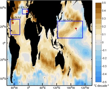
Global SST Trends. 1981–2015 SST trends from the optimum interpolated SST data set (OISST, https://www.ncdc.noaa.gov/oisst). Location of the oceanographic time‐series HOTS, BATS, and SATS in the study areas of the North Pacific subtropical gyre (sg‐NPac) and subtropical gyre North Atlantic (sg‐NAtl) as defined in McClain et al. [2004] based on dynamic height, and in the midlatitudes of the Eastern North Atlantic (ml‐ENA) as in Somavilla et al. [2016], where MLD long‐term trends will be shown later in the paper.

Certainly, the marked seasonality in the heat exchange with the atmosphere (summer heat uptake versus winter heat release) drives the broadly noticed coupled changes at seasonal time‐scales between the increase/decrease in upper water temperature and stratification, as well as their control in the extent of vertical mixing, nutrient supply to the upper layers, and primary productivity [Lozier et al., 2011]. However, as also noticed by Lozier et al. [2011], the long‐term variability of these processes is not necessarily dominated by the same driving forces. Indeed, the ocean stratification and mixing control from the overlying atmosphere is representative of processes governing the evolution of parameters within and above the seasonal pycnocline, a feature that is created and destroyed annually by definition. It is the permanent pycnocline which acts as a barrier layer against turbulent mixing [Sprintall and Cronin, 2011] and prevents the ocean from being progressively mixed from the top to the bottom. The properties of the permanent pycnocline are controlled by air‐sea exchanges at mid and high‐latitudes at mode water formation places and their annual subduction rate since it is this flux that ventilates the permanent pycnocline. Thus, temperature and salinity anomalies generated by winter air‐sea exchanges at these locations are carried at depth by ocean currents to remote locations where from below they exert control over the permanent pycnocline [Cronin and Sprintall, 2011]. As a consequence, unlike the atmospherically driven control on stratification of the seasonal pycnocline from above, the permanent stratification of the water column is sustained from below by ocean circulation.

Bearing that in mind, the assumption that ocean surface warming is unequivocally associated with a more stratified and less mixed ocean seems inaccurate. The existence of such a definitive relation is commonly supported by model outputs projecting increased near‐surface stratification and shallower mixed layers under global warming scenarios [Behrenfeld et al., 2006; Polovina et al., 2008; Boyce et al., 2010; Tyrrell, 2011; Gruber, 2011; Capotondi et al., 2012; Schmidtko et al., 2017]. However, CMIP5 models have shown difficulties in reproducing the MLD seasonal cycle and the location of the maximum MLDs in the Southern Ocean [Sallée et al., 2013]. The seasonal cycle of the mixed layer at midlatitude areas of thick mixed layers is intimately related to, and critically controlling, the ventilation of the permanent pycnocline [Marshall and Nurser, 1993]. This causes any inaccuracy in determining the location of maximum MLDs and the MLD seasonal cycle to misrepresent the thermohaline properties of the permanent pycnocline and its ventilation rates [Sallée et al., 2013]. These biases are not specific only to the Southern Ocean, and CMIP5 simulations have generally been found affected by large drifts in circulation and stratification from mid to high‐latitudes [Russell et al., 2015], which call into question the presumed unequivocal relation between warming, increasing stratification, and shallower MLDs.

It seems evident that increased stratification from surface warming and freshening would hinder the ventilation of the ocean. However, the ventilation of the ocean depends on a second competing force, wind‐driven divergence that can compensate and even reverse the effects of ocean warming from above causing increased stratification [Russell et al., 2006; Lauderdale et al., 2013]. Apart from the certain warming of the upper ocean over the last 30 years [Alexander et al., 2013], the poleward intensification of the westerly winds in the Southern Ocean is one of the most significant trends in the global climate system [Russell et al., 2006; Sallée et al., 2010]. In the Northern Hemisphere, a poleward migration of the jet stream (maximum westerlies) has also been found but in this case associated with a weaker and wavier (higher wave amplitude) jet stream [Archer and Caldeira, 2008; Capua and Coumou, 2016]. Both the poleward migration and the wave amplitude and asymmetry changes of the jet stream may result in wind‐driven divergence changes [Lauderdale et al., 2013; Landschützer et al., 2015]. On the other hand, the weakening of the jet stream has been related to a higher frequency of atmospheric blocking anomalies in the Northern Hemisphere [Barnes, 2013; Francis and Vavrus, 2012] which can have severe effects on the upper ocean vertical structure and ocean circulation [Somavilla et al., 2016]. All these changes have an effect on MLD and stratification variability that may oppose the expected one‐directional changes due to a regular warming from the overlying atmosphere.

Here we derive from hydrographic data the MLD and stratification trends observed in the upper ocean surface layer. In contrast to model simulations, we find that while SST increases in every area studied at midlatitudes, stratification either increases or decreases, and MLD deepens with enhanced deepening of winter MLDs. We present these results in section 3. The reasons behind these results and their consequences for biogeochemistry are discussed in section 4, focusing on: (1) caveats regarding the assumption that a warmer ocean will be more stratified and the suitability of the density difference between the surface and 200 m, the most widely used stratification index, to represent the tendency of a water column to be mixed (section 4.1); (2) the roles of changes in the buoyancy forcing (densification of the ocean surface due to cooling and/or evaporation) and wind‐driven divergence/convergence (Ekman pumping) on MLD deepening trends (section 4.2); and (3) the potential effects of our findings on primary productivity and ocean oxygenation (section 4.3).

2. Material and Methods

2.1. Study Areas and Data Sources

The study focuses on the long‐term changes and trends in Mixed Layer Depth (MLD) and stratification in the subtropical gyres and midlatitude regions of the North Atlantic and North Pacific in the areas shown in Figure 1. These areas are of particular interest because ocean warming is observed there and has been related to reduced primary productivity and ocean deoxygenation through increased stratification and shallower MLDs [Behrenfeld et al., 2006; Polovina et al., 2008; Boyce et al., 2010; Talley et al., 2016] and/or they comprise or partially overlap with mode water formation regions. Besides, in each of these areas, long‐term oceanographic time series are also regularly maintained providing high‐quality hydrographic data, which make feasible assessments of actual long‐term changes in ocean stratification and MLD. Oceanographic time‐series used are the time series at ocean observatories HOTS (http://hahana.soest.hawaii.edu/hot/, $22.8°$ N, $158°$ W) in the North Pacific subtropical gyre (sg‐NPac); BATS (http://bats.bios.edu/ $32.2°$ N, $64.5°$ W) in the North Atlantic subtropical gyre (sg‐NAtl); and SATS (http://www.boya-agl.st.ieo.es/, $43.8°$ N, $3.8°$ W) at midlatitudes of the eastern North Atlantic (ml‐ENA). A caveat of using standard oceanographic time‐series is that they can be affected by temporal gaps and provide local conditions for only a single spot, and so may not be consistently representative of a wider region. To overcome this issue, we combine them with other data sets that provide greater temporal and spatial coverage (Argo floats, global gridded ocean reanalysis, and satellite data).

To assess changes in MLD and stratification, we use the density profiles from the oceanographic time‐series, Argo floats, and ocean reanalysis (ECMWF Ocean Reanalysis System 4, ORAS4) [Balmaseda et al., 2013a]. To evaluate the warming of the ocean surface, data of sea surface temperature (SST) based mainly on satellite data (OISST, https://www.ncdc.noaa.gov/oisst) are used. To estimate the effects of buoyancy fluxes and Ekman pumping on MLD winter deepening, we use surface fluxes from NCEP/NCAR Reanalysis data set [Kalnay et al., 1996] (For further information on these data sets, see section 1.1 in supporting information). Our results would not change by using ECMWF Reanalysis data, since the comparison between NCEP/NCAR and ECMWF reanalysis data show very good agreement (the coefficient of variation of the RMSD is less than 3%).

2.2. Stratification and MLD Indexes

Stratification and MLD are among the most useful properties in oceanography because of their relevance both in climate processes and biogeochemical cycles. However, there are no standard criteria for their definitions and hence to establish objective metrics [González‐Pola et al., 2007; Thomson and Emery, 2014]. Figure 2 provides a view of different methods within a typical midlatitude winter profile and the problem of comparing methods for MLD determination when not perfectly homogeneous mixed layers exist (www.mldidentificationexperiment.com)—in this case due to the existence of both a deep MLD and an evanescent shallow MLD. Figure 2 also shows two extreme hypothetical profiles with the same bulk overall stratification.

Figure 2.

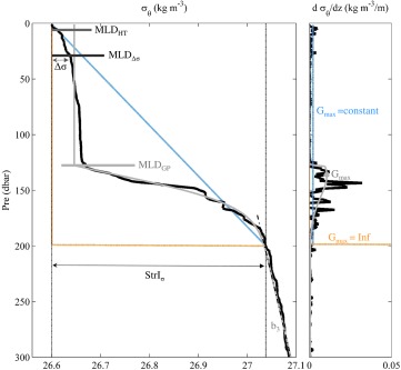
MLD and stratification quantification methods. (a) Density profile (black line) measured at SATS on the 19 December 2002 and its corresponding MLD _{Δ σ} ( $\Delta \sigma$ = 0.03 $\text{kg}\hspace{0.17em}{\mathrm{m}}^{-3}$), MLD_HT, and $Str{I}_{\sigma }$ estimations. The grey line shows the best fit of the density profile based on Gonzalez‐Pola et al. [2007] to a prescribed functional form and the MLD_GP obtained from that fit. The slope of the permanent pycnocline obtained from that fit, b ₃, is highligted by the dash black line. The blue and orange profiles show extreme (academic) cases of profiles with identical density difference between the surface and 200 m ( $Str{I}_{\sigma }$) to the actual profile measured at SATS on the 19 December 2002, but one with this density difference concentrated at a specific depth (step‐like profile, orange profile) and the other with this density difference uniformly distributed from the surface to 200 m (continuous type profile, blue profile, MLD absent). (b) Density change per meter of the water (dσ/dz) showing the maximum stratification of the profile (Gmax) based on the fit to the density profile following the Gonzalez‐Pola et al. [2007] algorithm.

The temperature ( $Str{I}_{\theta }$) or density ( $Str{I}_{\sigma }$) difference between the sea surface and 200 m is the stratification index that is most frequently employed [Behrenfeld et al., 2006; Capotondi et al., 2012]. The MLD is often estimated using the so‐called threshold methods, which define the MLD as the depth at which temperature or density differs from the surface value by a given amount ( $\Delta \theta$ or $\Delta {\sigma }_{\theta }$) (Figure 2). Alternatively, the use of other more advanced metrics for MLD determination is not rare. Here, we include the measures of MLD obtained following the Gonzalez‐Pola et al. [2007] algorithm (MLD_GP) and the Holte and Talley [2009] algorithm (MLD_HT). The Gonzalez‐Pola et al. [2007] algorithm is based on the best fit of density profiles to a predefined “ideal” functional form (i.e., converting the actual profile to an analytical curve). This fitting depends on various parameters with physical meaning among which is the MLD (MLD_GP in Figure 2) and from which also various measures of stratification can be obtained. The most representative are the slope of the permanent pycnocline, denoted by b ₃, and the maximum stratification of each profile, G _max, i.e., the maximum density increase per meter in the water column in the profile (Figure 2b). Since both temperature and salinity data are available in the data sets used in this study, we focus on the density‐based estimates of these methods.

2.3. Trends and Seasonality in the Upper Ocean

Long‐term changes and trends in signals like SST, stratification, and MLD having clear, well‐defined seasonal signals can be analyzed through well‐established statistical tools. If we expect a smooth variation, a good approach is the assumption that the data can be modeled by a periodic signal and optionally a linear trend. This will be the case of SST and $Str{I}_{\sigma }$. Through a harmonic fit, a periodic signal can be approximated by:

$$y(t)=\underset{\text{linear} \text{trend}}{\underbrace{a_0+a_{1}t}}+\underset{\text{seasonal} \text{cycle}}{\underbrace{a_2\cos (2\pi t)+a_3\sin (2\pi t)+a_4\cos (4\pi t)+a_5\sin (4\pi t)}}$$ (1)

where time is in decimal years. This mixed model corresponds to a linear trend plus annual and semiannual harmonics. The parameters are then fitted by generalized least squares method and the inclusion/exclusion of more parameters in the fitting is determined by a t test [Jenkins and Watts, 1998].

For the MLD a fitting using harmonics is unsatisfactory, as the mean evolution shows a discontinuity from the maximum MLD reached at the end of the winter to the surface at the beginning of the spring (Figure 3b). Moreover, between the end of the winter and beginning of spring, the MLD can alternate from very deep to very shallow values when incipient stratification is established at the surface (Figure 3b). Actually, at times a deep but vanishing MLD and a shallow incipient MLD coexist. Since this transition period marks the end of the winter and beginning of the spring, we establish this day as the date of minimum climatological SST when on average the maximum MLD is reached (±5.33 days). Centered on the SST Date _min, we define after visual inspection the period of time when the MLD is not unequivocally defined with a range of $0.1\hspace{0.17em}\text{year}$ ( $0.05\hspace{0.17em}\text{year}$ to each side) (Figure 3b). During this time of the year, in order to avoid underestimation of the climatological maximum MLD due to evanescent very shallow MLDs that occur under transient calm conditions, we retain for the fitting only the maximum MLD reached each year during this period (filled circles in Figure 3b). Using these data, the climatological seasonal cycle of the MLD is fitted by using a polynomial of third degree, as done by Gonzalez‐Pola et al. [2007] (the orange line in Figure 3c). If we had used all available data instead, the maximum winter MLD would be biased toward the shallower values in the range of deepest MLDs reached at the end of the winter (Figure 3c). In order to explore trends, this exclusion of transient shallow MLDs does not make a difference.

Figure 3.

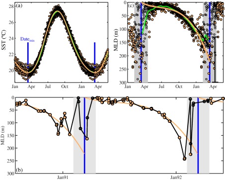
SST and MLD climatological seasonal cycles. (a) SST available data (orange‐filled circles) in the $4°$ ×  $4°$ box centered at the position of BATS oceanographic time‐series in the sg‐NAtl and its corresponding climatological seasonal cycle through Fourier decomposition (orange line) and biweekly averaging (green). (b) MLD temporal evolution at BATS oceanographic time‐series from September 1990 to May 1992. The blue vertical lines mark the date of minimum climatological SST at that location (Date _min in Figure 3a) and the grey shadow area the MLD‐undefined period during which the MLD alternates from very deep to very shallow values. The filled orange circles during the MLD‐undefined period show the maximum MLD reached during this period each corresponding year. Filled orange circles from each year represent the data that are retained for MLD climatological cycle fitting. (c) Following this criteria, all MLD estimations available at BATS from 1990 to 2015. The climatological seasonal cycle of the MLD obtained using the orange‐filled circles is shown by the orange line. Using all available data (orange‐filled circles + open circles), the climatological seasonal cycle of the MLD follows the black line. The brace bracket indicates the range of deepest MLDs reached at the end of the winter. The green line shows the MLD climatological seasonal cycle from biweekly averaging.

Climatological seasonal cycles are also commonly obtained from weekly, biweekly, or monthly average values. For signals with a smooth variation like SST or $Str{I}_{\sigma }$, the differences among these approaches are not particularly crucial when a large amount of data are available (i.e., both curves almost overlap, Figure 3a), but for the MLD the use of such averages may introduce important deviations and artifacts. As shown in Figure 3c, this approach provides a maximum winter MLD biased toward the shallowest value in the range of deepest MLDs reached at the end of the winter and artificially introduces a shallowing of the MLD during the period when the MLD is not unequivocally defined. Such shallowing as a physical process may occasionally occur, but in general the MLD simply alternates between very shallow and deep values (Figure 3b).

MLD long‐term trends are calculated as linear regression of MLD anomaly time‐series. This anomaly time‐series is the sequence of observed minus fitted seasonal cycle values. Regarding the ocean ventilation and ocean productivity, the winter conditions are especially relevant, so we also calculate the winter and summer MLD long‐term trends. These are calculated as linear regression of winter and summer MLD anomalies against time (e.g., only MLD anomalies during the winter (December, January, and February) or the summer (June, July, and August) are retained for the regression).

2.4. Winter MLD Trends and Its Forcing

In addition to the analysis of the long‐term changes and trends, we investigate the role of the different drivers of winter MLD variability. Destabilizing buoyancy forcing from cooling and/or evaporation making the ocean surface colder and saltier induces convective mixing of surface water with deeper water. Wind stirring always causes vertical turbulence in the upper mixed layer; however, it is less effective than convective mixing to thicken the mixed layer, and the autumn‐winter mixed layer deepening is controlled by the buoyancy forcing [Kantha and Clayson, 2000; Alexander et al., 2000; Somavilla et al., 2011]. Because the ocean mixed layer responds so rapidly to surface densification by buoyancy‐forced processes, the deepening of the mixed layer can often be estimated successfully using one‐dimensional approaches as the nonpenetrative convection equation [Marshall and Schott, 1999]:

$$h={\left[\frac{2{\displaystyle {\int }_{t_0}^{t_f}{B}_0}dt}{N^2}\right]}^{1/2}$$ (2)

where the vertical extent of the mixed layer (h, MLD) results from the integration in time of the buoyancy forcing (B ₀) assuming the water column stratification (N ², Brunt‐Vaisala frequency) has a constant value with depth. Using this expression, the expected changes in winter MLD in each of the study areas according to changes in (i) winter buoyancy fluxes estimated from NCEP/NCAR reanalysis data and (ii) stratification observed in oceanographic time‐series are calculated (for detailed information, see section 1.2.1 in supporting information).

Horizontal convergences/divergences of the water masses due to wind stress curl generate downward/upward nonturbulent vertical velocities that pump (Ekman pumping) the upper ocean surface layer. This pumping generates a vertical displacement of the interface that defines the base of the mixed layer, displacement that thickens mixed layers in convergent zones and thins in divergent zones [de Szoeke, 1980; Carranza and Gille, 2015]. The effects of vertical advection due to Ekman pumping on winter MLD are considered here by calculating the vertical velocities (w_EK) resulting from horizontal convergences/divergences of the water masses due to wind stress (τ) curl using NCEP/NCAR reanalysis data (positive wEK generates downwelling and thickening the MLD, and negative wEK upwelling and thining of the MLD) (for detailed information, see section 1.2.2. in supporting information).

3. Results

3.1. SST, Stratification, and MLD Seasonal Cycles

As introduced above, our paper focuses on MLD and stratification long‐term changes at midlatitude ocean basins of the Northern Hemisphere. Before addressing this main topic, we briefly consider the ability of the different data sources and methods for representing the amplitudes and phases of the MLD and stratification seasonal cycles for the different study areas.

The time series of SST, stratification measured as $Str{I}_{\sigma }$, and MLD in the subtropical gyres of the North Pacific (sg‐NPac) and North Atlantic (sg‐NAtl) and in the midlatitudes of the eastern North Atlantic (ml‐ENA) show, as expected, marked seasonal cycles (Figure 4). For SST and $Str{I}_{\sigma }$, the cycles start to increase at the beginning of spring after reaching their annual minima. They continue increasing until the end of the summer when they reach their maxima and decrease in autumn and winter until they reach again their annual minima. Conversely to SST and stratification, the MLD evolution does not have a smooth annual cycle. Its annual cycle starts at the surface at the beginning of spring, remains more or less stable during late spring and summer, and deepens progressively during autumn and winter until the deepest MLD is reached before any distinct signature vanishes. The days of maximum and minimum climatological MLD are, therefore, consecutive. A shallowing of the MLD is not observed as SST and $Str{I}_{\sigma }$ increase, and the MLD actually deepens slowly during late spring and summer. In Figure 4 only MLD_GP is shown but climatological seasonal cycles from MLD_HT and MLD ${}_{\Delta \sigma }$ show similar results (supporting information Figure S2). This agreement among MLD determination methods is also found for long‐term changes presented in the next section. In order to avoid redundancy of results and considering that the Gonzalez‐Pola et al. [2007] algorithm additionally provides information of the upper ocean vertical structure and stratification that will be used in the discussion, we will not show the figures for MLD_HT and MLD ${}_{\Delta \sigma }$ here. These can be found in supporting information.

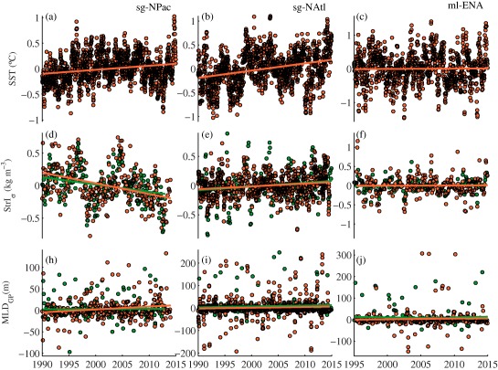
Figure 4.

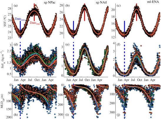
SST, stratification, and MLD climatological seasonal cycles. (a), (b), and (c) 1990–2015 OISST available data (orange filled circles) in $4°$ ×  $4°$ boxes centered at the position of oceanographic time‐series in the sg‐NPac, sg‐NAtl, and ml‐ENA, respectively, and their corresponding climatological seasonal cycles (orange line). (d), (e), and (f) Stratification measured as StrI_σ on oceanographic time‐series (orange‐filled circles), and in $4°$ ×  $4°$ boxes centered at the locations of oceanographic time‐series from ORAS4 ocean reanalysis data (green circles), and Argo floats (blue circles). The climatological seasonal cycles using the oceanographic time‐series, ORAS4, and Argo floats data are shown by the orange, green, and blue lines, respectively. (g), (h), and (i) idem to (d), (e) and (f) but for MLD_GP. The vertical blue lines mark the date of minimum SST at each location and the red ones the date of maximum SST.

The minimum and maximum values of the climatological seasonal cycles of SST from OISST, $Str{I}_{\sigma }$ and the different MLDs indexes estimated from oceanographic time‐series and the dates when they are reached (Date _min and Date _max) are summarized in Table 1 (similar tables for estimates from ORAS4 and Argo floats time‐series are summarized in supporting information Tables S1 and S2). For SST, the highest temperatures are reached in the sg‐NPac ( $25.58°\mathrm{C}$) while the lowest temperatures and greatest amplitude of the seasonal cycle are found in the ml‐ENA (between $12.66°\mathrm{C}$ and $20.14°\mathrm{C}$). For stratification measured as $Str{I}_{\sigma }$, the greatest values and amplitude are reached in the sg‐NAtl (between $0.14\hspace{0.17em}$ and $2.84\hspace{0.17em}\text{kg}\hspace{0.17em}{\mathrm{m}}^{-3}$) and the lowest in the ml‐ENA ( $0.12\hspace{0.17em}\text{kg}\hspace{0.17em}{\mathrm{m}}^{-3}$). The climatological MLD seasonal cycles measured as MLD_GP from oceanographic time‐series range between the surface and approximately 100 m in the sg‐NPac, 220 m in the sg‐NAtl, and 180 m in the ml‐ENA (Figure 4 and Table 1). Thus, climatologically, the deepest winter MLDs are found in the sg‐NAtl.

Table 1.

Maximum and Minimum Values of Climatological Seasonal Cycles and the Dates When They are Reached ( $Dat{e}_{\text{min}})$ and $Dat{e}_{\text{max}})$, Respectively From Oceanographic Time‐Series in the Subtropical Gyres of the North Pacific (sg‐NPac) and North Atlantic (sg‐NAtl), and in the Midlatitudes of the Eastern North Atlantic (ml‐ENA)

	sg‐NPac		sg‐NAtl		ml‐ENA
	Min (Datemin)	Max (Datemax)	Min (Datemin)	Max (Datemax)	(Min Datemin)	Max (Datemax)
SST, StrIσ, and MLDGP shown in Figure 4
SST ( ${}^{°}\mathrm{C}$)	23.64 (23 Feb)	25.58 (24 Aug)	19.71 (12 Mar)	24.4 (21 Aug)	12.66 (3 Mar)	20.14 (18 Aug)
StrIσ ( $\text{kg}\hspace{0.17em}{\mathrm{m}}^{-3}$)	1.16 (27 Feb)	2.11 (15 Sep)	0.14 (16 Mar)	2.84 (21 Aug)	0.12 (6 Mar)	2.06 (20 Aug)
MLDGP ( $\mathrm{m}$)	0	99.8	0	222.2	0	184.23
Additional MLD estimations shown in supporting information Figure S2
MLDHT ( $\mathrm{m}$)	0	72.05	0	174.91	0	187.09
MLD Δ σ ( $\mathrm{m}$)	0	75.11	0	210.64	0	207.45

Despite the different spatial and temporal resolution of oceanographic time‐series, ocean reanalysis, and Argo floats, the amplitude of the $Str{I}_{\sigma }$ seasonal cycles from the different data sources differs by less than 6% (see Table 1 and supporting information Tables S1 and S2) showing also similar phases as seen in Figure 4. For MLDs, just considering the seasonal cycles from observations and ORAS4, their amplitudes differ by less than 4% for MLD_GP, 10% for MLD_HT, and 5% for MLD ${}_{\Delta \sigma }$. It is interesting to highlight that the climatological maximum winter MLDs estimated with Argo floats are on average 30 m deeper than estimated on oceanographic time‐series or ocean reanalysis independently of the method used for the MLD determination. Possible explanations for this difference could be the different sampling period or the lower vertical resolution. The vertical resolution of Argo floats in the depth range of climatological maximum MLDs (between 100 and 250 m) is approximately of 20 m, smaller than the 30 m difference between climatological maximum winter MLDs in observations and Argo floats. On the other hand, the estimation of the climatological seasonal cycles from observations for the sampling period of Argo floats (2003–2015) gives a climatological maximum MLD that is 20 m deeper than for the period 1990–2015. Thus, using the same sampling period, the difference between the climatological maximum winter MLDs from observations and Argo is reduced to 10 m, which is within the expected uncertainty due to the lower vertical resolution of Argo floats. From this, we rule out that the different vertical resolution is responsible for the 30 m deeper climatological maximum MLDs in Argo floats and conclude that it is due to their different, later sampling period.

3.2. SST, $Str{I}_{\sigma }$, and MLD Long‐Term Changes and Trends

Long‐term changes and trends are analyzed over SST, $Str{I}_{\sigma }$, and MLD anomaly time‐series (Figure 5). Anomaly time‐series are obtained as the difference between observed and fitted climatological seasonal cycle values. As shown in the previous section, the different data sources reproduce adequately the climatological seasonal cycles, and so we rely on them for the investigation of low‐frequency changes.

Figure 5.

SST, stratification, and MLD long‐term changes. (a), (b), and (c) 1990–2015 OISST anomaly time‐series in $4°$ ×  $4°$ boxes centered at the position of oceanographic time‐series in the sg‐NPac, sg‐NAtl, and ml‐ENA, respectively, and their linear trends (line). (d), (e), and (f) StrI_σ anomaly time‐series estimated on oceanographic time‐series (orange‐filled circles) and in $4°$ ×  $4°$ boxes centered at the locations of oceanographic time‐series from ORAS4 ocean reanalysis data (green circles). The linear trends using the oceanographic time‐series and ORAS4 data are shown by the orange and green lines, respectively. (g), (h), and (i) idem to (d), (e) and (f) but for MLD_GP anomaly time‐series.

Low‐frequency changes derived from oceanographic and reanalysis time‐series seem consistent, and this inference is supported by similar long‐term trends obtained from both data sources. Data from Argo floats are not shown in Figure 5 since they do not span the same sampling period, and the trends obtained are not comparable with those from ocean observations and reanalysis data.

SST warming trends are found in all the three oceanic areas. The warming trends in the sg‐NPac and sg‐NAtl are of $0.09$ and $0.15°\mathrm{C}\hspace{0.17em}\hspace{0.17em}{\text{decade}}^{-1}$, respectively. Both trends are significant at 0.05 significance level and are within the average in the global ocean ( $0.09$– $0.13°\mathrm{C}\hspace{0.17em}\hspace{0.17em}{\text{decade}}^{-1}$ in the upper 75 m) [Alexander et al., 2013]. In the ml‐ENA, the surface warming is less pronounced ( $0.03°\mathrm{C}\hspace{0.17em}\hspace{0.17em}{\text{decade}}^{-1}$) due to intense cooling events associated with the occurrence of winter blocking events since 2005 in the area [Somavilla et al., 2009, 2011, 2016] that were not compensated by a slight summer temperature increase. Concurrent with surface warming, stratification measured as $Str{I}_{\sigma }$ is observed showing increasing trends in the sg‐NAtl ( $+0.05\hspace{0.17em}\text{kg}\hspace{0.17em}{\mathrm{m}}^{-3}\hspace{0.17em}{\text{decade}}^{-1}$) but also decreasing trends in the sg‐NPac ( $-0.16\hspace{0.17em}\text{kg}\hspace{0.17em}{\mathrm{m}}^{-3}\hspace{0.17em}{\text{decade}}^{-1}$). The moderate surface warming in the ml‐ENA coincides with relatively moderate changes in $Str{I}_{\sigma }$ ( $+0.004\hspace{0.17em}\text{kg}\hspace{0.17em}{\mathrm{m}}^{-3}\hspace{0.17em}{\text{decade}}^{-1}$)‐1 order of magnitude lower than that observed in the sg‐NAtl.

Regarding the MLD long‐term changes, MLD deepening trends ranging from $1\hspace{0.17em}$ to $8\hspace{0.17em}\mathrm{m}\hspace{0.17em}\hspace{0.17em}{\text{decade}}^{-1}$ are found at the three sites (Figure 5) and by all three different MLD determination methods MLD_GP, MLD_HT, and MLD ${}_{\Delta \sigma }$ (Figure 5 and supporting information S2). Mostly due to the alternation of very deep to very shallow values of the MLD between the end of the winter and beginning of the spring (see section 2.3), the anomaly time‐series are very noisy. Still the trends are significant both in ocean observations and reanalysis data except for the ml‐ENA, and this can be more easily recognized on the MLD time‐series shown in Figure 6 with the trend shown by the white line. The deepening trends in the sg‐NPc and sg‐NAtl are consistent in ocean observations and ORAS4 reanalysis data and significant at 0.05 significance level (Table 2). In the ml‐ENA, deepening trends are found in ocean observations by the three MLD determination methods $ML{D}_{\Delta \theta }$, MLD_GP, MLD_HT (Table 2), but they are not significant and are not found in ORAS4 reanalysis data.

Figure 6.

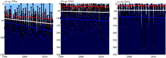
Winter versus Summer MLD long‐term trends. (a), (b), and (c) MLD temporal evolution estimated on hydrographic profiles at HOTS (sg‐NPac), BATS (sg‐NAtl), and SATS (ml‐ENA) oceanographic time‐series. The white lines represent the MLD long‐term trends calculated as linear regression of MLD anomaly time‐series against time shown by orange lines in Figure 5 (g), (h), and (i). The blue and red lines represent, respectively, the winter and summer MLD long‐term trends calculated as linear regression of MLD anomalies against time using only the winter (blue circles) or summer (red circles) data. With explanatory purposes, the trends (white, blue and red lines) ‐although calculated as linear regression of MLD anomaly time‐series against time‐ are made to vertically coincide with the actual average annual, winter or summer MLDs observed at each of these sites (white, blue, and red dots), summing up to the long‐term trends the corresponding long‐term average value (e.g: winter mean value for winter MLD trends or summer mean value for summer MLD trends). The waters above/below the MLD are shown in light/dark blue.

Table 2.

Linear Trends in SST, StrI_σ, and MLD Found in Observations From Oceanographic Time‐Series of the Subtropical Gyres of the North Pacific (sg‐NPac) and North Atlantic (sg‐NAtl), and in the Midlatitudes of the Eastern North Atlantic (ml‐ENA)

	sg‐NPac	sg‐NAtl	ml‐ENA
SST, StrIσ, and MLDGP trends shown in Figure 5
SST $(°\mathrm{C}\hspace{0.17em}\hspace{0.17em}{\text{decade}}^{-1})$	0.09 ± 0.01	0.15 ± 0.02	0.03 ± 0.01
StrIσ ( $\text{kg}\hspace{0.17em}{\mathrm{m}}^{-3},{\text{decade}}^{-1}$)	−0.16 ± 0.04	0.05 ± 0.01	0.004 ± 0.04
MLDGP ( $\mathrm{m},{\text{decade}}^{-1}$)	6.8 ± 2.1	4.3 ± 1.7	0.8 ± 4
Additional MLD estimations shown in supporting information Figure S3
MLDHT ( $\mathrm{m},{\text{decade}}^{-1}$)	4.3 ± 1.7	3.3 ± 1.8	4.7 ± 5
MLD Δ σ ( $\mathrm{m},{\text{decade}}^{-1}$)	7.1 ± 2.1	4.9± 1.8	8.8 ± 9
Winter MLD trends in Figure 6
MLDGP ( $\mathrm{m},{\text{decade}}^{-1}$)	16.9 ± 5.1	10.6 ± 4.8	9 ± 4
MLDHT ( $\mathrm{m},{\text{decade}}^{-1}$)	10.9 ± 4.2	15.8 ± 5.1	22.1 ± 5
MLD Δ σ ( $\mathrm{m},{\text{decade}}^{-1}$)	16 ± 5.2	16 ± 4.9	−3.5 ± 20
Summer MLD trends in Figure 6
MLDGP ( $\mathrm{m},{\text{decade}}^{-1}$)	2 ± 2	−0.8 ± 0.5	0.18 ± 1.9
MLDHT ( $\mathrm{m},{\text{decade}}^{-1}$)	0.15 ± 2.4	−3.71 ± 2.3	−1.67 ± 0.5
MLD Δ σ ( $\mathrm{m},{\text{decade}}^{-1}$)	1.5 ± 5.2	−0.1 ± 1.2	0.81 ± 1.5

Separately, due to the crucial role of deep winter MLDs in ocean ventilation and global biogeochemical cycles, we also investigate the winter MLD long‐term trends. As shown in Figure 6 and summarized in Table 2, winter MLDs are getting deeper at rates between 2.5 and 5 times faster than the annual trends. The faster winter MLD deepening is found for all three study areas by all three MLD determination methods. However, winter MLD deepening trends are again significant only in the sg‐NPac and sg‐NAtl, not in the ml‐ENA data. In view of Figure 6c, in the ml‐ENA rather than a trend, a jump toward much deeper winter MLDs is observed from 2005 onward when intense cooling events occurred in the area [Somavilla et al.,2009, 2016]. Unlike the winter MLDs, summer MLDs are deepening 2.5–5 times slower than the annual trends; MLDs are even getting shallower in the case of the sg‐NAtl (Table 2). Thus, the winter MLD deepening trends at rates between 10 and $17\hspace{0.17em}\mathrm{m}\hspace{0.17em}\hspace{0.17em}{\text{decade}}^{-1}$ dominate the MLD deepening trends.

Argo floats trends cannot be used to provide further support to the trends in oceanographic time‐series and ocean reanalysis. However, the finding of climatological maximum winter MLDs on average 30 m deeper when estimated from Argo floats than from the oceanographic time‐series or the ocean reanalysis is nevertheless indicative of progressively deeper winter MLDs. As explained in the previous section, this finding cannot be explained by the different vertical resolution of Argo data and seems to be due to its shorter and more recent period of sampling (2003–2015).

Overall, the finding of warmer and deeper MLDs relies on the estimation of MLDs by several objective methods from hydrographic profiles both from long‐term hydrographic time‐series and ocean reanalysis; this finding is consistent with Argo floats within the period of overlap. Accordingly, it should not be attributable to a particular methodology or only noticeable at specific oceanic stations. The maps of MLD long‐term trends in the sg‐NPac, sg‐NAtl, and ml‐ENA in Figure 7 confirm that the MLD deepening trends found at the location of oceanographic time‐series by the different data sources and determination methods are representative of larger oceanic regions.

Figure 7.

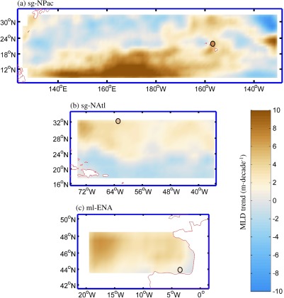
MLD deepening trends in the sg‐NPac, sg‐NAtl, and ml‐ENA. 1990–2015 MLD (MLD_GP) deepening trends from ORAS4 ocean reanalysis data in the regions of the sg‐NPac, sg‐NAtl, and ml‐ENA delimited in Figure 1. The MLD deepening trends from oceanographic time‐series in each of these regions is shown by the colored circles (its color indicates the MLD deepening trend according to the color scale). Figure 7 is smoothed with a 2 × 2 2‐D digital filter.

4. Discussion

4.1. $Str{I}_{\sigma }$: A Good Measure of Stratification?

Based mainly on model results, ocean surface warming is commonly associated with increased stratification and shallower mixed layers. In contrast to this assumption, we find that stratification is not unequivocally increasing, and MLD is not shoaling, despite evident and substantial ocean warming.

The results from the climatological seasonal cycles calculated here also do not support the widespread idea that the warmer the ocean surface, the shallower the mixed layer. During spring and summer stabilizing buoyancy forcing from heating—causing the ocean surface to become warmer—stratifies the surface and isolates it from the deeper waters [Cronin and Sprintall, 2011]. Thus, stabilizing buoyancy forcing hinders upper ocean mixing, and during the summer months wind‐induced mixing controls the vertical extension of the mixed layer [Alexander et al., 2000; Kantha and Clayson, 2000; Somavilla et al., 2011]. Since different processes govern the variabilities of SST and MLD during summer months, MLD does not necessarily shoal as SST and $Str{I}_{\sigma }$ increase; MLD remains more or less stable during late spring and summer. Consequently, the apparent shallowing of the MLD found in MLD climatological seasonal cycles obtained from weekly, biweekly, or monthly averaging (Figure 3c and section 2.3) cannot be explained by physical process of buoyancy and wind forcing. Such shallowing and climatological maximum MLDs shallower than actually observed—artefact of the data processing and averaging—have important implications when estimating the nutrient replenishment due to winter mixing and the onset of the spring bloom [Sallée et al., 2015; Llort et al., 2015].

It is true that during autumn‐winter destabilizing buoyancy forcing from cooling makes the ocean surface colder and the MLD deeper through convective mixing. However, the comparison of the different climatological seasonal cycles shows that the lowest temperature and the minimum stratification values ( $Str{I}_{\sigma }$) at the end of the winter are in the ml‐ENA but not the climatological deepest winter MLD which is found in the sg‐NAtl. SST is often used as index of physical changes within the surface mixed layer including its vertical extension, having been used to identify permanently stratified zones [Behrenfeld et al., 2006, 2008; O'Malley et al., 2010; González Taboada and Anadón, 2014] characterized by low primary productivity. However, this approach has been reported to be subjected to several caveats, since SST changes cannot be solely attributed to shoaling or deepening of the MLD at synoptic scales and is influenced by mesoscale processes and horizontal advection [Carranza and Gille, 2015; Dave and Lozier, 2015].

Similarly, the finding of surface warming concurrent with decreasing stratification measured as $Str{I}_{\sigma }$ in the sg‐NPac is not surprising (Figure 5). The commonly involved link between increasing stratification and surface warming trends is supported by the seasonal coupling between stabilizing buoyancy forcing from atmospheric heating and the warming of the ocean surface that stratifies the upper layer. However, stabilizing/destabilizing buoyancy forcing not only occurs due to heating/cooling causing the ocean surface to become warmer/cooler but also due to precipitation/evaporation causing the ocean surface to become fresher/saltier [Cronin and Sprintall, 2011]. The study areas are subjected to changes in the evaporation‐precipitation balance [Alexander et al., 2013] that can compensate for the expected surface density decrease due to surface warming. This is observed in the sg‐NPac where surface density increase ( $0.08\hspace{0.17em}\text{kg}\hspace{0.17em}{\mathrm{m}}^{-3}\hspace{0.17em}{\text{decade}}^{-1}$) due to salinity changes ( $0.13\hspace{0.17em}{\text{decade}}^{-1}$) outpace the temperature contribution to making the surface waters lighter (for density and salinity the linear trends are also calculated through a harmonic fit as for SST and $Str{I}_{\sigma }$). At depth, however, salinity is decreasing ( $-0.012\hspace{0.17em}{\text{decade}}^{-1}$) making the waters at depth lighter ( $-0.02\hspace{0.17em}\text{kg}\hspace{0.17em}{\mathrm{m}}^{-3}\hspace{0.17em}{\text{decade}}^{-1}$), decreasing the density difference between the surface and 200 m ( $Str{I}_{\sigma }$) thought the ocean surface is warming. On the other hand, even with temperature changes dominating the density changes, the expected finding of increasing stratification concurrent with surface warming assumes that warming is faster at the ocean surface than at depth. The properties at depth are controlled from below through advective pathways of remotely formed water masses [Sprintall and Cronin, 2011]. Faster warming at water formation regions and changes in circulation can result in warming trends faster at depth than at the surface as observed in the ml‐ENA (not significant trend at the surface versus a warming trend at depth of $0.16°\mathrm{C}\hspace{0.17em}{\text{decade}}^{-1}$) [Somavilla et al., 2011]. A somewhat similar situation has been found in CMIP5 models under mitigation scenarios, when a transient imbalance between cooling at the ocean surface and continued warming in subsurface waters takes place [John et al., 2015].

Finally, the finding of increasing $Str{I}_{\sigma }$ trends concurrent with MLD deepening trends is perhaps more troubling. The index of stratification $Str{I}_{\sigma }$ shown in the above figures is the most widely used. However, beyond its simplicity, the rationale for its use is questionable. A good stratification index must represent a measure of the tendency of a water column to be mixed. The deepening of the mixed layer is inversely proportional to the density difference between the mixed layer and the water below it ( $\Delta {\sigma }_{bMLD}$) according to the equation for the time evolution of the turbulent kinetic energy (TKE) [Barton et al., 2015; Follows and Dutkiewicz, 2002]. With an identical density difference between the surface and 200 m, and so identical $Str{I}_{\sigma }$, will be more difficult to mix a water column with this density difference concentrated at a specific depth (step‐like profile in Figure 2, $\Delta {\sigma }_{bMLD}$ =  $Str{I}_{\sigma }$) than a water column with this density difference uniformly distributed from the surface to 200 m (continuous type profile in Figure 2, $\Delta {\sigma }_{bMLD}$ =  $Str{I}_{\sigma }/200\hspace{0.17em}\mathrm{m}$). In other words, the same forcing from wind and cooling will mix deeper the water column in which the density difference between the surface and the 200 m level is evenly distributed than the one in which the same density difference is concentrated at a specific depth. Thus, a good stratification index requires information about the vertical distribution of the density difference between the surface and the deeper layers that $Str{I}_{\sigma }$ does not include.

The search for a stratification index that provides better representation of the tendency of a water column to being mixed needs to consider all kinds of stratification situations that can be found in the ocean, from strongly to very weakly stratified areas. Such a specific study is clearly beyond the scope of this study, which is focussed on midlatitude ocean regions. As a preliminary analysis (results not shown), we have examined three stratification indexes that quantify in different ways the vertical distribution of the density difference between the surface mixed layer and the waters below. These alternative stratification indexes are: the maximum stratification of the water column, G _max (Figure 2b); the slope of the steepness, b ₃ (Figure 2a); and the potential energy $\mathrm{\Phi }$ criteria that integrates the vertical density distribution [Simpson et al., 1977; Huret et al., 2013]. Note that these different stratification indexes do not measure the same feature of the upper ocean vertical structure. Hence, we do not find agreement of results regarding the stratification seasonal cycles and trends from these indexes, unlike MLD (in which the different determination methods all try to estimate the vertical extent of the mixed layer). G _max temporal variability is dominated by its seasonal cycle as for SST and $Str{I}_{\sigma }$. On the other hand, b ₃ and $\mathrm{\Phi }$ show distinct, low‐frequency variability resembling that depicted from winter MLDs at the three study areas. While G _max and $Str{I}_{\sigma }$ seem indexes representing the stratification of the seasonal pycnocline, b ₃ and $\mathrm{\Phi }$ seem to be more representative of the stratification through the permanent pycnocline. Thus, our analysis from midlatitudes does not allow us to identify one stratification index as clearly better than the others. For that purpose, a global study that considers all kind of stratification situations that can be found in the ocean is necessary.

4.2. Winter MLD Deepening Trends and Their Forcing

In the previous section, we explained why ocean warming does not necessarily imply an increase of stratification and why changes in stratification measured as $Str{I}_{\sigma }$ should not be expected to reliably inform about changes in the vertical extent of mixing. However, we still have to provide an explanation for the observed MLD deepening trends. Deepening MLD trends seem to be mostly driven by the faster trends of winter MLDs. We discuss here the roles of changes in the buoyancy forcing (densification of the ocean surface due to cooling and/or evaporation) and wind‐driven divergence/convergence (Ekman pumping) on winter MLD deepening trends. In order to facilitate the understanding of this discussion, we first briefly describe the limitations of these estimates. A schematic of the processes considered is shown in Figure 8.

Figure 8.

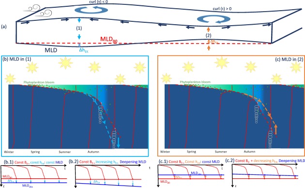
Schematic of buoyancy forcing (B ₀) and Ekman pumping ( $\Delta h_{Ek}$) effects on MLD winter deepening. (a) Enhanced deepening of the MLD generated by downward pumping of the surface layer in water mass convergent areas (1) versus attenuation deepening of the MLD due to upward pumping in divergent regions (2) due to wind‐stress curl with respect to the expected MLD from a particular B ₀ ( $ML{D}_{B0}$). (b) and (c) Effects of B ₀ and ( $\Delta h_{Ek}$) on MLD temporal evolution in water mass (1) convergent and (2) divergent regions. The expected MLD from B ₀ ( $ML{D}_{B0}$) is identical in Figures 8b and 8c, but the downwards (b) and upwards (c) w_Ek integrated throughout the winter make the observed MLD (MLD_obs) deeper than ( $ML{D}_{B0}$) in Figure 8b and shallower in Figure 8c. No changes in stratification, B ₀, and $\Delta h_{Ek}$ make the MLD to be constant in time ((b.1) and (c.1)). An increase of downward $\Delta h_{Ek}$ in convergent zones (b.2) or a decrease of the upward $\Delta h_{Ek}$ in divergent zones (c.2) can make the MLD deeper with time without the need of changes in stratification and/or B ₀.

The expected changes in winter MLD in every study area due to changes in (1) winter buoyancy fluxes (B ₀) estimated from NCEP/NCAR reanalysis data and (2) stratification (N ²) observed in oceanographic time‐series are calculated according to the non‐penetrative convection equation [Marshall and Schott, 1999] (equation (2)). Although winter mixing is mostly governed by the accumulated effect of buoyancy (heat) loss throughout the winter, extraordinary convection episodes appear more likely to occur when heat loss is concentrated in intense mixing events, rather than distributed evenly but more weakly throughout the winter [Marshall and Schott, 1999; Vage et al., 2008; Somavilla et al., 2011]. The time integration of B ₀ used in equation (2) does not allow us to reproduce specific events deviating largely from the long‐term mean value of winter MLDs. However, we are not interested in explaining specific years but the long‐term changes, and this expression seems to provide plausible estimations of the MLD long‐term mean and trends as argued below.

Additionally, we calculate the enhanced deepening/shoaling of winter MLD that can occur in downwelling/upwelling regions due to changes in the Ekman pumping. Basically, we calculate the vertical velocities (w_EK) from horizontal convergences and divergences of the water masses due to wind stress curl using the NCEP/NCAR reanalysis data and integrate throughout the winter the resulting vertical displacement ( $\Delta h_{EK}$) that this pumping generates (Figures 8b and 8c). Vertical velocities due to Ekman pumping and the resulting vertical displacement of MLD may seem small and without effect on MLD variability (e.g., daily average of w_EK = 3.5 ${10}^{-6}\hspace{0.17em}\mathrm{m}\hspace{0.17em}{\mathrm{s}}^{-1}$ and $\Delta h_{EK}$ = 0.3 $\mathrm{m}$). However, at seasonal time‐scales the effects of Ekman pumping on MLD variability are noticeable and when integrated (accumulated) throughout the winter can drive the MLD to be tens of meters deeper than expected from the buoyancy forcing in convergent zones and vice versa in divergent zones [de Szoeke, 1980] (Figure 8a).

With all that in mind, the lower plots of Figure 9 show that changes in the buoyancy forcing and stratification included in the non‐penetrative equation do not completely explain winter MLD trends since the trends estimated from the buoyancy forcing (red lines in Figures 9h, 9i and 9j) do not coincide with the observed ones (blue lines). The average difference between the line observed and the line estimated from the buoyancy forcing seems to coincide in each study area with the expected integrated vertical displacement due to Ekman pumping ( $\Delta h_{Ek}$) (Figures 9a and 9c) (in other words, adding the estimated effect of Ekman pumping displaces the red line to coincide with the observed blue line, Figures 8b1 and c1). Thus, in the sg‐NAtl area the average winter $\Delta h_{Ek}$ is $-23\hspace{0.17em}\mathrm{m}$ (Figures 9c and 9f) coinciding approximately with the downwards displacement of 27 m that would make the mean winter MLD estimated from buoyancy forcing (165 m) to reach the average value found in the observations (192 m) (Figure 9i). In the sg‐NPac, the average winter $\Delta h_{Ek}$ within the HOTS station location is positive (+24 m) indicating that divergence is pushing the water column up in contrast to the rest of the subtropical gyre (Figures 9a and 9e). This value of winter $\Delta h_{Ek}$ is also in the range of the upward displacement of 37 m that would make the mean winter MLD estimated from buoyancy forcing (135 m) reach the average value found in the observations (98 m) (Figure 9h). In the ml‐ENA, observed and estimated trends from buoyancy fluxes almost overlap in the vertical, in agreement with no significant upward or downward $\Delta h_{Ek}$ in the area (Figure 9c).

Figure 9.

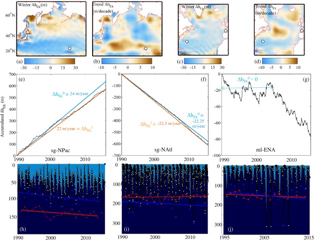
Contributions of buoyancy forcing (B ₀) and Ekman pumping ( $\Delta h_{Ek}$) to MLD winter deepening. (a) and (c) Integrated vertical displacement throughout the winter (Winter $\Delta h_{Ek}$ (m)) due to winter average w_EK in the North Pacific and North Atlantic, respectively. (b) and (d) Trends of winter $\Delta h_{Ek}$ ( $\mathrm{m},{\text{decade}}^{-1}$) in both basins. The white circles indicate the positions of the oceanographic time‐series in the sg‐NPac, sg‐Natl, and ml‐ENA. (e), (f), and (g) Accumulated $\Delta h_{Ek}$ over time at the position of oceanographic time‐series in the sg‐NPac, sg‐NAtl, and ml‐ENA. Constant $\Delta h_{Ek}$ per year able to generate the accumulated $\Delta h_{Ek}$ in the sg‐NPac and sg‐NAtl are shown by the blue and orange lines. The blue ones indicate the constant $\Delta h_{Ek}$ per year observed at the beginning of the time series ( $\Delta h_{Ek}^0$) and the orange ones at the end ( $\Delta h_{Ek}^f$). (h), (i), and (j) MLD time‐series. The red circles indicate the estimated depth of the MLD at the end of the winter from B ₀ (h) and the red line its trend. The blue lines show winter MLD deepening trends found in observations.

In the sg‐NAtl, the downward velocities are increasing, and so the integrated downward displacement through the winter is also increasing, at a rate of $7.6\hspace{0.17em}\mathrm{m} \hspace{0.17em}{\text{decade}}^{-1}$ (Figures 9d and 9f). This compensates and outpaces the expected shallowing of MLD due to changes in the buoyancy forcing and stratification ( $-1.1\hspace{0.17em}\mathrm{m} \hspace{0.17em}{\text{decade}}^{-1}$, red line in Figure 9i) enabling the MLD to deepen with time as observed (situation scheme Figure 8b2). In the sg‐NPac, upward w_Ek are decreasing (Figures 9b and 9e), contributing to the faster deepening trends found in observations ( $16\hspace{0.17em}\mathrm{m}\hspace{0.17em}\hspace{0.17em}{\text{decade}}^{-1}$) with respect to the deepening MLD trends expected from changes in the buoyancy forcing and stratification ( $7.8\hspace{0.17em}\mathrm{m}\hspace{0.17em}\hspace{0.17em}{\text{decade}}^{-1}$) (situation scheme Figure 8c2). In the ml‐ENA, as observed for winter MLDs, rather than a trend a regime shift is observed after 2005 (Figure 9g) in correspondence with the severe changes in the vertical extent of mixing in the area.

Evidence of the relationship between winter MLD variability and changes in that season's air‐sea heat and salt exchanges (buoyancy forcing) is common in the literature [Carton et al, 2008; Vage et al., 2008; Somavilla et al., 2011] but the relationship of long‐term changes in MLD with changes in the Ekman pumping has not been recognized. However, changes in wind patterns including a poleward migration and wave amplitude and asymmetry changes of the maximum westerlies in both Northern and Southern hemispheres that may result in such changes in wind‐driven divergence and Ekman pumping have been extensively reported [Russell et al., 2006; Sallée et al., 2010; Archer and Caldeira, 2008; Capua and Coumou, 2016]. Similarly, circulation changes in the subtropical gyres estimated from Sea Surface Height (SSH) that are a reflection of Ekman pumping changes have also been described [McClain et al., 2004; Roemmich et al., 2007]. The maps of average winter vertical displacement due to Ekman pumping ( $\Delta h_{Ek}$) shown in Figure 9a and c are consistent with those found in the literature for both the Atlantic and the Pacific [Marshall and Nurser, 1993; Qiu and Huang, 1995]. Besides, the estimated deepening trends of the MLD due to Ekman pumping (∼ $7\hspace{0.17em}\mathrm{m}\hspace{0.17em}\hspace{0.17em}{\text{decade}}^{-1}$) are similar to those found for the Atlantic and Pacific from SSH changes. The $+0.5\hspace{0.17em}\text{cm}\hspace{0.17em}{\text{yr}}^{-1}$ SSH (η) trends found in these areas would be equivalent to a $5\hspace{0.17em}\mathrm{m}\hspace{0.17em}\hspace{0.17em}{\text{decade}}^{-1}$ deepening of the pycnocline (D) according to the expression $g\prime D^2/2f=g{\eta }^2/2fg\prime$ where f is the Coriolis parameter and g' the reduced gravity (∼ ${10}^{-2}\mathrm{m}\hspace{0.17em}{\mathrm{s}}^{-2}$) [McClain et al., 2004]. These trends due to Ekman pumping are not usually applied to the MLD. However, since they pump the entire upper layer vertical structure, they inevitably also affect the MLD, as shown in this study, being able to enhance, compensate, and even outpace the effects of ocean warming and increasing stratification on MLD deepening trends.

Overall, changes in the buoyancy forcing and stratification considered in the non‐penetrative equation together with wind‐driven divergence changes provide an explanation for the finding of deepening winter MLD trends concurrent with surface warming in the three study areas. Applying the nonpenetrative equation for N ² constant over time (the long‐term average value of N ² in each study area), the estimated winter MLD trends would be of $1.1\hspace{0.17em}\mathrm{m}\hspace{0.17em}\hspace{0.17em}{\text{decade}}^{-1}$ in the sg‐NPac (versus $7.8\hspace{0.17em}\mathrm{m}\hspace{0.17em}\hspace{0.17em}{\text{decade}}^{-1}$ considering changes in stratification); $5\hspace{0.17em}\mathrm{m}\hspace{0.17em}\hspace{0.17em}{\text{decade}}^{-1}$ in the sg‐NAtl (versus $-1.1\hspace{0.17em}\mathrm{m}\hspace{0.17em}\hspace{0.17em}{\text{decade}}^{-1}$ considering changes in stratification); and $10\hspace{0.17em}\mathrm{m}\hspace{0.17em}\hspace{0.17em}{\text{decade}}^{-1}$ in the ml‐ENA versus ( $9\hspace{0.17em}\mathrm{m}\hspace{0.17em}\hspace{0.17em}{\text{decade}}^{-1}$ considering changes in stratification). Thus, both changes in the horizontal convergences/divergences of the water masses due to wind stress curl (circulation) and in the buoyancy forcing contribute to deepening the winter MLDs in all the three areas. Changes in stratification seem to modulate the response of the upper ocean to the atmospheric forcing, enhancing deepening trends in the sg‐NPac and damping them in the sg‐NAtl.

4.3. Biogeochemical Implications

According to our findings, ocean observations do not support an unequivocal relation between ocean surface warming, increasing stratification, and shallower MLDs. The existence of such a link in model simulations under global warming scenarios has been extensively used to explain observed or projected declines in global oceanic oxygen content and primary productivity [Behrenfeld et al., 2006; Polovina et al., 2008; Boyce et al., 2010; Tyrrell, 2011; Gruber, 2011; Capotondi et al., 2012; Schmidtko et al., 2017]. How do our findings reconcile deepening MLDs with the observation of less productive and oxygenated oceans?

Global satellite observations have been widely used to document the existence of an inverse relationship between changes in SST and surface phytoplankton chlorophyll concentrations (a proxy for phytoplankton biomass). However, rather than being a universal relationship, it seems to be restricted to satellite observations for specific areas [see e.g., Ramírez et al., 2017, supporting information Figure S1] and time‐scales of variability. As pointed by Lozier et al. [2011], ocean surface warming, increasing stratification, and reduced primary productivity are linked by the “straightforward” relationship existing between the physical processes and primary productivity at seasonal time‐scales. The problem is that no such relationship exists at longer, decadal time‐scales [Lozier et al., 2011]. Besides, it has been shown that global‐scale correlations between upper ocean stratification and chlorophyll a are driven by strong associations between the two properties in the central and western equatorial Pacific [Dave and Lozier, 2013], and that these correlations are not due to SST changes but result from the advection of heat, salt, and nutrients in the region [Dave and Lozier, 2015].

In situ primary production observations also do not support such a definitive relationship either: increases of primary production have been found concurrent with surface warming trends at BATS and HOTS oceanic stations [Wallhead et al., 2014; Saba et al., 2010; Corno et al., 2007]. Interestingly, biogeochemical ocean general circulation models were tested to reproduce this finding, and only one of twelve models compared for each site was able to reproduce an increase of primary production concurrent with the surface warming trends [Saba et al., 2010]. The deeper winter‐time MLDs and more temperate nature of the ecosystems were proposed as possible explanations for the low skill of the models [Saba et al., 2010].

The origin of these findings of increasing primary production together with surface warming trends from specific oceanic stations [Wallhead et al., 2014; Saba et al., 2010; Corno et al., 2007] has been used to claim that the station data cannot necessarily be extrapolated to larger spatial scales. However, we have demonstrated that the finding of warmer and deeper MLDs in long‐term oceanographic time‐series is representative of larger oceanic areas, and so it can also be the case for their effects on the availability of nutrients and primary productivity. The net effect of deepening winter MLDs on the nutrient supply to the euphotic zone enhancing primary productivity depends on the drivers of this deepening. Deepening winter MLDs as a result of intensified buoyancy losses and/or weaker stratification would increase convective mixing and so entrainment of nutrient‐rich deep waters into the upper layer. This nutrient enhancement is expected to be accompanied by an increase in primary production. Deepening winter MLDs due to changed wind‐driven divergence would not necessarily entrain more nutrient rich deep waters into the upper layer, since the Ekman pumping would push the whole water column down, not solely the MLD. Just the maintenance of the nutrient supply may lead to an increase of primary production in a warmer upper ocean under the assumption of a bottom‐up control and nutrient‐limited production. However, in this case a dilution effect on phytoplankton due to deeper MLDs should be also considered. In agreement with these expectations, in the vicinity of HOTS oceanographic time‐series, where winter MLD deepening trend is more strongly dominated by changes in the buoyancy forcing and stratification, the enhancement of nutrient supply, and primary production is larger than at BATS oceanographic time‐series [Saba et al., 2010].

Recently, the discrepancy between satellite and in situ phytoplankton biomass observations at global scales has been examined, showing that contemporary relationships between chlorophyll changes and ocean warming are not indicative of proportional changes in productivity, as light‐driven decreases in chlorophyll can be associated with constant or even increased photosynthesis [Behrenfeld et al., 2016]. Still this explanation seems to implicitly require the occurrence of shallower MLDs to cause the light‐driven decreases in chlorophyll concurrent with surface warming. As explained through this paper, warmer MLDs are not necessarily shallower, and further investigation is needed.

The global oceanic oxygen content decline detected over the past few decades has been attributed in ocean models, and so in observations, to warming‐induced declines in oxygen solubility, and reduced ventilation of deeper waters from enhanced upper‐ocean stratification [Helm et al., 2011; Schmidtko et al., 2017]. However, our results do not necessarily contradict the finding of oceans losing breath, because these results may indicate that ventilation increases for warmer waters which have lower capacity to contain dissolved gasses, including oxygen. The oxygen decline in this case should be similar to the oxygen decrease due to warming‐induced solubility losses since ventilation is not reduced. Interestingly, Schmidtko et al. [2017] found the oxygen decline in the depth range of mode waters ( $300$– $700\hspace{0.17em}\mathrm{m}$)—to which the midlatitudes areas of the ml‐ENA and sg‐NAtl would contribute to ventilate—coinciding with the expected decrease solely due to solubility changes. The waters above and below this depth range show oxygen declines larger than the expected decrease due to solubility changes that are attributed to reduced ventilation.

5. Conclusions

We have shown that surface warming is not definitively linked to a more stratified ocean with shallower mixed layers. The previously assumed relationship between increasing stratification and surface warming assumes that warming is faster at the ocean surface than at depth which is not necessarily the case, as found here for the midlatitudes of the Eastern North Atlantic. On the other hand, even when warming is faster at the surface, salinity changes can compensate for the expected surface density decrease due to surface warming. Moreover, even when the density difference between surface waters and those at depth increases, MLD can get deeper with time. The vertical extent of mixing depends not only on stratification but also on wind‐driven divergence and buoyancy losses. These can compensate for and outpace the effects on MLD of ocean warming and increasing stratification. Changes in both wind‐driven divergence and in the buoyancy forcing have been found to contribute to deepening the winter MLDs at the three study areas at midlatitudes considered in this work.

Overall, we have found that while SST increases at three study areas at midlatitudes, stratification both increases and decreases, and MLD deepens with enhanced deepening of winter MLDs at rates from 10 to 17 m decade⁻¹. These results rely on the estimation of several MLD and stratification indexes of different complexity from hydrographic profiles collected by long‐term oceanographic time‐series, by ocean reanalysis and by Argo floats. Because of the multiple data sources, the apparent deepening of winter MLDs cannot be attributed to a particular methodology or a specific oceanic station. Instead of that, the finding of warmer and deeper MLDs is representative of large oceanic regions and the likely mechanism could operate in other ocean regions [Martinez et al., 2016]. These conclusions may be extended to the expected enhancement of the nutrient availability and primary productivity due to deeper MLDs. Besides, warmer and deeper MLDs may indicate that subsurface waters are ventilated more with warmer waters which have lower capacity to contain dissolved gasses providing an alternative explanation for the oceanic oxygen content decline in some regions as midlatitudes areas of mode water formation.

Finally, it must be repeated that caution must be taken when using the density difference between the sea surface and 200 m ( $Str{I}_{\sigma }$) as stratification index. $Str{I}_{\sigma }$ is the most widely used stratification index, but it does not provides a good representation of the tendency of a water column to be mixed since it does not inform about the vertical distribution of the density difference between the surface and the deeper layers.

Supporting information

Supporting Information S1

Somavilla, R. , González‐Pola C., and Fernández‐Diaz J. (2017), The warmer the ocean surface, the shallower the mixed layer. How much of this is true?, J. Geophys. Res. Oceans, 122, 7698–7716, doi:10.1002/2017JC013125.

References

- Alexander, M. A. , Scott J. D., and Deser C. (2000), Processes that influence sea surface temperature and ocean mixed layer depth variability in a coupled model, J. Geophys. Res., 105(C7), 16,823–16,842. [Google Scholar]
- Archer, C. , and Caldeira K. (2008), Historical trends in the jet streams, Geophys. Res. Lett., 35, L08803, doi:10.1029/2008GL033614. [Google Scholar]
- Balmaseda, Mogensen M. A. K., and Weaver A. (2013a), Evaluation of the ECMWF ocean reanalysis system ORAS4, Q. J. R. Meteorol. Soc., 139, 1132–1161, doi:10.1002/qj.2063. [Google Scholar]
- Balmaseda, M. A. , Trenberth K. E., and K E. llén (2013b), Distinctive climate signals in reanalysis of global ocean heat content, Geophys. Res. Lett., 40, 1754–1759, doi:10.1002/grl.50382. [Google Scholar]
- Barnes, E. A. (2013), Revisiting the evidence linking arctic amplification to extreme weather in midlatitudes, Geophys. Res. Lett., 40, 4728–4733, doi:10.1002/grl.50880. [Google Scholar]
- Barton, A. D. , Lozier S. M., and Williams R. G. (2015), Physical controls of variability in North Atlantic phytoplankton communities, Limnol. Oceanogr., 60(1), 181–197, doi:10.1002/lno.10011. [Google Scholar]
- Behrenfeld, M. J. , O'Malley R. T., Siegel D. A., McClain C. R., Sarmiento J. L., Feldman G. C., Milligan A. J., Falkowski P. G., Letelier R. M., and Boss E. S. (2006), Climate‐driven trends in contemporary ocean productivity, Nature, 444(7120), 752–755, doi:10.1038/nature05317. [DOI] [PubMed] [Google Scholar]
- Behrenfeld, M. J. , Siegel D. A., and O'Malley R. T. (2008), Global ocean phytoplankton and productivity [in State of the climate in 2007], Bull. Am. Meteorol. Soc., 89, S56–S61, doi:10.1175/BAMS-89-7-StateoftheClimate. [Google Scholar]
- Behrenfeld, M. J. , O'Malley R. T., Boss E. S., Westberry T. K., Graff J. R., Halsey K. H., Milligan A. J., Siegel D. A., and Brown M. B. (2016), Revaluating ocean warming impacts on global phytoplankton, Nat. Clim. Change, 6(3), 323–330, doi:10.1038/nclimate2838. [Google Scholar]
- Boyce, D. G. , Lewis M. R., and Worm B. (2010), Global phytoplankton decline over the past century, Nature, 466(7306), 591–596, doi:10.1038/nature09268. [DOI] [PubMed] [Google Scholar]
- Capotondi, A. , Alexander M. A., Bond N. A., Curchitser E. N., and Scott J. D. (2012), Enhanced upper ocean stratification with climate change in the CMIP3 models, J. Geophys. Res., 117, C04031, doi:10.1029/2011JC007409. [Google Scholar]
- Capua, G. , and Coumou D. (2016), Changes in meandering of the Northern Hemisphere circulation, Environ. Res. Lett., 11(9), 094,028, doi:10.1088/1748-9326/11/9/094028. [Google Scholar]
- Carranza, M. M. , and Gille S. T. (2015), Southern Ocean wind‐driven entrainment enhances satellite chlorophyll‐a through the summer, J. Geophys. Res. Oceans, 120, 304–323, doi:10.1002/2014JC010203. [Google Scholar]
- Carton, J. A. , Grodsky S. A., and Liu H. (2008), Variability of the oceanic mixed layer, 1960–2004, J. Clim., 21(5), 1029–1047, doi:10.1175/2007JCLI1798.1. [Google Scholar]
- Corno, G. , Karl D. M., Church M. J., Letelier R. M., Lukas R., Bidigare R. R., and Abbott M. R. (2007), Impact of climate forcing on ecosystem processes in the North Pacific subtropical gyre, J. Geophys. Res., 112, C04021, doi:10.1029/2006JC003730. [Google Scholar]
- Cronin, M. F. , and Sprintall J. (2011), Wind and buoyancy‐forced upper ocean, in Encyclopedia of Ocean Sciences, edited by Steele J. H., Thorpe S. A., and Turekian K. K., pp. 327–345, Academic, San Diego, Calif. [Google Scholar]
- Dave, A. C. , and Lozier M. S. (2013), Examining the global record of interannual variability in stratification and marine productivity in the low‐attitude and midlatitude ocean, J. Geophys. Res. Oceans, 118, 3114–3127, doi:10.1002/jgrc.20224. [Google Scholar]
- Dave, A. C. , and Lozier M. S. (2015), The impact of advection on stratification and chlorophyll variability in the equatorial Pacific, Geophys. Res. Lett., 42, 4523–4531, doi:10.1002/2015GL063290. [Google Scholar]
- de Szoeke, R. A. (1980), On the effects of horizontal variability of wind stress on the dynamics of the ocean mixed layer, J. Phys. Oceanogr., 10, 1439–1454. [Google Scholar]
- Follows, M. , and Dutkiewicz S. (2002), Meteteorological modulation of the North Atlantic spring bloom, Deep Sea Res., Part II, 49, 321–344. [Google Scholar]
- Francis, J. A. , and Vavrus S. J. (2012), Evidence linking arctic amplification to extreme weather in midlatitudes, Geophys. Res. Lett., 39, L06801, doi:10.1029/2012GL051000. [Google Scholar]
- González‐Pola, C. , Fernández‐Diaz J. M., and Lavín A. (2007), Vertical structure of the upper ocean from profiles fitted to physically consistent functional forms, Deep Sea Res., Part I, 54(11), 1985–2004, doi:10.1016/j.dsr.2007.08.007. [Google Scholar]
- González Taboada, F. , and Anadón R. (2014), Seasonality of North Atlantic phytoplankton from space: Impact of environmental forcing on a changing phenology (1998–2012), Global Change Biol., 20(3), 698–712, doi:10.1111/gcb.12352. [DOI] [PubMed] [Google Scholar]
- Gruber, N. (2011), Warming up, turning sour, losing breath: Ocean biogeochemistry under global change, Philos. Trans. R. Soc. A, 369(1943), 1980–1996, doi:10.1098/rsta.2011.0003. [DOI] [PubMed] [Google Scholar]
- Helm, K. , Bindoff N., and Church J. (2011), Observed decreases in oxygen content of the global ocean, Geophys. Res. Lett., 38, L23602, doi:10.1029/2011GL049513. [Google Scholar]
- Holte, J. , and Talley L. (2009), A new algorithm for finding mixed layer depths with applications to Argo data and subantarctic mode water formation*, J. Atmos. Oceanic Technol., 26(9), 1920–1939, doi:10.1175/2009jtecho543.1. [Google Scholar]
- Huret, M. , Sourisseau M., Petitgas P., Struski C., Léger F., and Lazure P. (2013), A multi‐decadal hindcast of a physical‐biogeochemical model and derived oceanographic indices in the Bay of Biscay, J. Mar. Syst., 109, S77–S94, doi:10.1016/j.jmarsys.2012.02.009. [Google Scholar]
- IPCC . (2013), Climate Change 2013: The Physical Science Basis, in Working group I Contribution to the IPCC Fifth Assessment Report [Available at www.ipcc.ch/report/ar5/wg1/.]
- Jenkins, G. M. , and Watts D. G. (1998), Spectral Analysis and Its Applications, 5th ed., Emerson‐Adams Press, Boca Ratón, Fla. [Google Scholar]
- John, J. , Stock C., and Dunne J. (2015), A more productive, but different, ocean after mitigation, Geophys. Res. Lett., 42, 9836–9845, doi:10.1002/2015GL066160. [Google Scholar]
- Kalnay, E. , et al. (1996), The NCEP/NCAR 40‐year reanalysis project, Bull. Am. Meteorol. Soc., 77(3), 437–471, doi:10.1175/1520-0477(1996)077⟨0437:TNYRP⟩2.0.CO;2. [Google Scholar]
- Kantha, L. H. , and Clayson C. A. (2000), Small Scale Processes in Geophysical Fluid Flows, International Geophysics, vol. 67, Academic, New York. [Google Scholar]
- Landschützer, P. , et al. (2015), The reinvigoration of the Southern Ocean carbon sink, Science, 349(6253), 1221–1224, doi:10.1126/science.aab2620. [DOI] [PubMed] [Google Scholar]
- Lauderdale, J. , Garabato A., Oliver K., Follows M., and Williams R. (2013), Wind‐driven changes in Southern Ocean residual circulation, ocean carbon reservoirs and atmospheric CO2, Clim Dyn., 41(7–8), 2145–2164, doi:10.1007/s00382-012-1650-3. [Google Scholar]
- Llort, J. , Lévy M., Sallée J., and Tagliabue A. (2015), Onset, intensification, and decline of phytoplankton blooms in the Southern Ocean, ICES J. Mar. Sci., 72(6), 1971–1984, doi:10.1093/icesjms/fsv053. [Google Scholar]
- Lozier, S. M. , Dave A. C., Palter J. B., Gerber L. M., and Barber R. T. (2011), On the relationship between stratification and primary productivity in the North Atlantic, Geophys. Res. Lett., 38, L18609, doi:10.1029/2011GL049414. [Google Scholar]
- Marshall, J. , and Nurser G. (1993), Inferring the subduction rate and period over the North Atlantic, J. Phys. Oceanogr., 23, 1315–1329. [Google Scholar]
- Marshall, J. , and Schott F. (1999), Open‐ocean convection: Observations, theory, and models, Rev. Geophys., 37(1), 1–64. [Google Scholar]
- Martinez, E. , Raitsos D., and Antoine D. (2016), Warmer, deeper, and greener mixed layers in the North Atlantic subpolar gyre over the last 50 years, Global Change Biol., 22(2), 604–612, doi:10.1111/gcb.13100. [DOI] [PubMed] [Google Scholar]
- McClain, C. , Signorini S., and Christian J. (2004), Subtropical gyre variability observed by ocean‐color satellites, Deep Sea Res., Part I, 51(1–3), 281–301, doi:10.1016/j. dsr2.2003.08.002. [Google Scholar]
- O'Malley, R. T. , Behrenfeld M. J., Siegel D. A., and Maritorena S. (2010), Global ocean phytoplankton [in State of the climate in 2009], Bull. Am. Meteorol. Soc., 91, S75–S78, doi:10.1175/BAMS-91-7-StateoftheClimate. [Google Scholar]
- Polovina, J , Howell E. A., and Abecassis M. (2008), Ocean's least productive waters are expanding, Geophys. Res. Lett., 35, L03618, doi:10.1029/2007GL031745. [Google Scholar]
- Qiu, B. , and Huang R. X. (1995), Ventilation of the North Atlantic and North Pacific: Subduction versus obduction, J. Phys. Oceanogr., 25(10), 2374–2390, doi:10.1175/1520-0485(1995)025⟨2374:VOTNAA⟩2.0.CO;2. [Google Scholar]
- Ramírez, F. , Afán I., Davis L. S., and Chiaradia A. (2017), Climate impacts on global hot spots of marine biodiversity, Sci. Adv., 3(2), e1601,198, doi:10.1126/sciadv.1601198. [DOI] [PMC free article] [PubMed] [Google Scholar]
- Roemmich, D. , Gilson J., Davis R., Sutton P., Wijffels S., and Riser S. (2007), Decadal spin‐up of the South Pacific subtropical gyre, J. Phys. Oceanogr., 37(2), 162–173, doi:10.1175/JPO3004.1. [Google Scholar]
- Roemmich, D. , Church J., Gilson J., Monselesan D., Sutton P., and Wijffels S. (2015), Unabated planetary warming and its ocean structure since 2006, Nat. Clim. Change, 5(3), 240–245, doi:10.1038/nclimate2513. [Google Scholar]
- Russell, J. , Dixon K., Gnanadesikan A., Stouffer R., and Toggweiler J. (2006), The Southern hemisphere westerlies in a warming world: Propping open the door to the deep ocean, J Clim., 19(24), 6382–6390, doi:10.1175/JCLI3984.1. [Google Scholar]
- Russell, J. , Benway H., Bracco A., Deutsch C., Ito T., Kamenkovich I., and Patterson M. (2015), Ocean's Carbon and Heat Uptake: Uncertainties and Metrics, in US CLIVAR Rep, vol. 3, edited by K. Uhlenbrock, p. 33, U.S. CLIVAR Project Off. [Google Scholar]
- Saba, V. , et al. (2010), Challenges of modeling depth‐integrated marine primary productivity over multiple decades: A case study at BATS and HOT, Global Biogeochem. Cycles, 24, GB3020, doi:10.1029/2009GB003655. [Google Scholar]
- Sallée, J. , Speer K., Rintoul S., Sallée J., Speer K., and Rintoul S. (2010), Zonally asymmetric response of the Southern Ocean mixed‐layer depth to the southern annular mode, Nat. Geosci., 3, 273–279, doi:10.1038/ngeo812. [Google Scholar]
- Sallée, J. , et al. (2013), Assessment of Southern Ocean mixed layer depths in CMIP5 models: Historical bias and forcing response, J. Geophys. Res. Oceans, 118, 1845–1862, doi:10.1002/jgrc.20157. [Google Scholar]
- Sallée, J. , Llort J., Tagliabue A., and Lévy M. (2015), Characterization of distinct bloom phenology regimes in the Southern Ocean, ICES J. Mar. Sci., 72(6), 1985–1998, doi:10.1093/icesjms/fsv069. [Google Scholar]
- Schmidtko, S. , Stramma L., and Visbeck M. (2017), Decline in global oceanic oxygen content during the past five decades, Nature, 542(7641), 335–339, doi:10.1038/nature21399. [DOI] [PubMed] [Google Scholar]
- Simpson, J. H. , Hughes D. G., and Morris N. C. G. (1977), The relation of seasonal stratification to tidal mixing on the continental shelf, Deep‐Sea Res., 24, 327–340. [Google Scholar]
- Somavilla, R. , González‐Pola C., Rodriguez C., Josey S. A., Sánchez R. F., and Lavín A. (2009), Large changes in the hydrographic structure of the Bay of Biscay after the extreme mixing of winter 2005, J. Geophys. Res., 114, C01001, doi:10.1029/2008JC004974. [Google Scholar]
- Somavilla, R. , González‐Pola C., Ruiz Villarreal M., and Lavín A. (2011), Mixed layer depth (MLD) variability in the southern Bay of Biscay. Deepening of winter MLDs concurrent to generalized upper water warming trends?, Ocean Dyn., 61(9), 1215–1235, doi:10.1007/s10236-011-0407-6. [Google Scholar]
- Somavilla, R. , González‐Pola C., Schauer U., and Budéus G. (2016), Mid‐2000s North Atlantic shift: Heat budget and circulation changes, Geophys. Res. Lett., 43, 2059–2068, doi:10.1002/2015GL067254. [DOI] [PMC free article] [PubMed] [Google Scholar]
- Sprintall, J. , and Cronin M. F. (2011), Upper ocean vertical structure, in Encyclopedia of Ocean Sciences, edited by Steele J. H., Thorpe S. A., and Turekian K. K., 2nd ed., pp. 217–224, Academic, San Diego, Calif. [Google Scholar]
- Talley, L. , et al. (2016), Changes in ocean heat, carbon content, and ventilation: A review of the first decade of GO‐SHIP global repeat hydrography, Annu. Rev. Mar. Sci., 8(1), 185–215, doi:10.1146/annurev-marine-052915-100829. [DOI] [PubMed] [Google Scholar]
- Thomson, R. E. , and Emery W. J. (2014), Chapter 4.11, in Data Analysis Methods in Physical Oceanography, 3rd. edn., pp. 313–424, Elsevier, Boston, Mass., doi:10.1016/B978-0-12-387782-6.00004-1.
- Tyrrell, T. (2011), Anthropogenic modification of the oceans, Philos. Trans. R. Soc. A, 369(1938), 887–908, doi:10.1098/rsta.2010.0334. [DOI] [PubMed] [Google Scholar]
- Vage, K. , Pickart R., Moore G., and Ribergaard M. (2008), Winter mixed‐layer development in the central Irminger Sea: The effect of strong, intermittent wind events, J. Phys. Oceanogr., 38, 541–565. [Google Scholar]
- Wallhead, P. J. , Garçon V. C., Casey J. R., and Lomas M. W. (2014), Long‐term variability of phytoplankton carbon biomass in the Sargasso Sea, Global Biogeochem. Cycles, 28, 825–841, doi:10.1002/2013GB004797. [Google Scholar]
Associated Data
This section collects any data citations, data availability statements, or supplementary materials included in this article.
Supplementary Materials