Predictive modeling of respiratory tumor motion for real-time prediction of baseline shifts

Abstract

Baseline shifts in respiratory patterns can result in significant spatiotemporal changes in patient anatomy (compared to that captured during simulation), in turn, causing geometric and dosimetric errors in the administration of thoracic and abdominal radiotherapy. We propose predictive modeling of the tumor motion trajectories for predicting a baseline shift ahead of its occurrence. The key idea is to use the features of the tumor motion trajectory over a 1 min window, and predict the occurrence of a baseline shift in the 5 s that immediately follow (lookahead window). In this study, we explored a preliminary trend-based analysis with multi-class annotations as well as a more focused binary classification analysis. In both analyses, a number of different inter-fraction and intra-fraction training strategies were studied, both offline as well as online, along with data sufficiency and skew compensation for class imbalances. The performance of different training strategies were compared across multiple machine learning classification algorithms, including nearest neighbor, Naïve Bayes, linear discriminant and ensemble Adaboost. The prediction performance is evaluated using metrics such as accuracy, precision, recall and the area under the curve (AUC) for repeater operating characteristics curve. The key results of the trend-based analysis indicate that (i) intra-fraction training strategies achieve highest prediction accuracies (90.5–91.4%); (ii) the predictive modeling yields lowest accuracies (50–60%) when the training data does not include any information from the test patient; (iii) the prediction latencies are as low as a few hundred milliseconds, and thus conducive for real-time prediction. The binary classification performance is promising, indicated by high AUCs (0.96–0.98). It also confirms the utility of prior data from previous patients, and also the necessity of training the classifier on some initial data from the new patient for reasonable prediction performance. The ability to predict a baseline shift with a sufficient lookahead window will enable clinical systems or even human users to hold the treatment beam in such situations, thereby reducing the probability of serious geometric and dosimetric errors.

1. Introduction

Effective management of respiratory motion is a critical aspect of thoracic and abdominal radiotherapy (Keall et al 2006). Owing to respiratory motion, tumors may receive less than the prescribed dose leading to local failure, or normal tissue and critical organs may receive more than intended dose, leading to increased toxicity. Such errors tend to have a greater impact in hypofractionated treatment regimens such as stereotactic body radiation therapy (SBRT) that involves the administration of high, biologically potent radiation doses in relatively few fractions (1–5 compared to 30–40 for conventionally fractionated regimens). To address the issue of intrafraction respiratory motion management, a number of real-time target position monitoring systems have been developed and made commercially available for sensing target position. These use a variety of technologies such as optical markers, surface photogrammetry, radioopaque implanted markers in combination with kilovoltage and/or megavoltage x-ray imaging, radiofrequency transponders, and ultrasound (Keall et al 2006). These systems typically output real-time 3D (translation only) or 6-degree-of-freedom (6DOF—translations and rotations) positional information of the tumor target. This information may then be used in a variety of interventional motion management strategies such as gating the radiation beam on/off, continuously following the tumor target with the radiation beam, known commonly as real-time tracking or a combination of the above two strategies, i.e. tracking within a pre-determined temporal or respiratory phase-based window.

Tumor motion tracking as well a real-time prediction of instantaneous tumor location have been extensively studied (Verma et al 2011, Vedam 2013, Lee and Motai 2014). The approaches discussed in such studies provide reasonably accurate estimates of short-term, quasi-periodic changes in tumor location, such as those seen due to respiratory motion. An outstanding issue in motion management is to handle long-term changes such as baseline drifts or sudden anomalous or irregular tumor motion due to sneezing or coughing. While realtime prediction is well-suited for modeling the tumor motion and continuously realigning the beam, the prediction look-ahead times reported so far largely fall under a second, while longer look-ahead times compromise on accuracy (Verma et al 2011). This limitation makes instantaneous location prediction inadequate for forecasting the occurrences of motion anomalies such as abrupt shifts, and mean position drift (or baseline shift).

A baseline shift is described as a period of irregular motion involving substantial displacement (temporary or permanent) in the mean position of the tumor. (See figure 1.) Such shifts can occur in lung cancer patients due to changes in the breathing pattern, between primarily chest breathing and primarily abdominal breathing. Increased interest in hypofractionated regimens such as lung stereotactic body radiotherapy (SBRT) has resulted in treatments with more beam directions (7–9 fields) and with more modulation using intensity modulated radiotherapy (IMRT). Treatment delivery of such regimens can take several minutes, over which baseline shifts can occur. For example, patients are often nervous during the initial part of the fraction and exhibit primarily chest breathing. When they eventually relax, they exhibit primarily abdominal breathing, potentially causing baseline shifts. These shifts can also manifest as gradual drifts in the respiratory motion.

Figure 1.

Baseline shifts as exhibited in three-dimensional motion trajectories recorded from lung cancer patients using the Synchrony system used as patient representative motion in this study (Suh et al 2008).

Several recent studies have investigated baseline shifts and their management. Pepin et al (2011) analyzed and evaluated several methods of dynamic gating for real-time baseline shift compensation. Tachibana et al (2011) presented a simple and flexible monitoring system for intrafractional patient movements and evaluated its utility for respiratory-gated treatment. However, to our knowledge, the potential of using predictive modeling of the tumor motion baseline for real-time prediction of imminent baseline shifts has not been well explored. In this work, we study baseline shift prediction with sufficient time before its occurrence, which can help automatic or manual beam-hold and, if necessary, patient realignment in order to reduce significant geometric and dosimetric errors. We propose using real-time prediction of baseline shifts (with an approximate lookahead window of 5 s) by modeling the trend characteristics of the tumor motion baseline. We study the characteristics of the tumor motion baseline in already observed data to facilitate prediction of baseline shifts ahead of their occurrence (see figure 2). Beyond the current scope, the eventual clinical translation of this technique will enable the system or, even a human user, to hold the beam when they observe a baseline shift. The lookahead window needs to be adequate for manual intervention by a therapist, especially in case of smaller centers or centers in developing regions of the world, which may not have access to the latest technology.

Figure 2.

Schematic showing proposed methodology for prediction of baseline shifts.

2. Methods

2.1. Dataset

For our study, we used lung tumor motion data modeled by the CyberKnife Synchrony system (Adler et al 1997), acquired previously at Georgetown University (Suh et al 2008) for 143 treatment fractions in 42 patients. The tumor motion is estimated from correlations between external on-body markers and internal fiducial markers implanted around, or sometimes within, the tumor mass, and monitored using periodic stereoscopic x-ray imaging. The data provide modeled 3D coordinate location of the tumor in time, documenting the tumor motion (in millimeters) along three dimensions—superior–inferior (SI), anterior–posterior (AP) and left–right (LR)—as a function of time. The validity of the estimated data has been discussed in previous works, with (Seppenwoolde et al 2007) finding the systematic error of position estimation to be less than 1 mm for all patients and mean 3D error to be less than 2 mm for 80% of the time. The mean and standard deviation of the 3D position estimation root mean square error documented in the dataset is 1.5 ± 0.8 mm. The sampling rate for the respiratory motion data is 25 samples per second. The overall mean respiratory period is 3.9 s (calculated over 143 treatment fractions in 42 patients). Therefore, an average respiratory cycle would approximately correspond to a 100 samples. The duration of treatment fractions in the dataset ranges from 5 min to 100 min (mean duration is approx. 30 min).

For the purposes of the analyses in this work, each treatment fraction is regarded as an independent record in order to diversify the training data made available for the classification algorithms. This assumption is made to capitalize on any variations in a patient’s breathing characteristics across treatment fractions, while allowing the prediction models to harness similarities among different patients’ data.

2.2. Baseline computation

Recent studies have employed different techniques to capture the baseline of the tumor motion trace, also referred to as the low-frequency, the non-periodic or the ultra-cyclic component of the respiratory motion of the tumor. In this study, we consider two techniques that have been used in previous works for mean position tracking.

For our trend-based analysis, we employ the locally weighted scatterplot smoothing (LOESS), which has been reported to be suitable for extracting tumor motion baselines (Ruan et al 2007). LOESS was chosen for the trend-based analysis due to its suitability in using local regression based smoothing to allow for comparison of stability between consecutive tumor motion segments. However, in case of the binary classification analysis, the baseline shift annotation criterion is more stringent with a ‘steadiness’ requirement before and after a baseline shift. In such scenario, the LOESS more than often fails to capture the important variations in the trajectories.

In our binary classification analyses, we employ the moving average for baseline computation. As reported by a number of studies (George et al 2008, Wilbert et al 2008, Yoon et al 2011), the moving average has been found to be optimal for reducing random noise by eliminating the systematic error due to non-stationary signals, while the motion of each respiration cycle is considered to be residual random error. The moving average thus ignores the instantaneous tumor location, but provides a loyal estimate of the general trend of tumor motion. A drawback of the moving average is the inherent latency introduced due to computation. This varies depending on the span of the computation range, and also the availability of future samples. However, in this study, the baseline computation latency is accounted for and is integrated into the look-ahead window for baseline shift prediction.

The baseline of the tumor motion thus computed using smoothing is then used for heuristic annotation of baseline shifts, as outlined in the next section. The use of the smoothed signal for the annotation of a motion segment ensures that the labeling is not affected by high frequency noise, but rather is influenced by and indicative of the predominant trend of the signal exhibited in that segment.

2.3. Heuristic based definition and annotation of baseline shifts

The dataset used in our analysis does not have any annotations corresponding to actual occurrences of motion anomalies and baseline shifts that could be used as prediction class labels. In order to facilitate predictive analysis on this data, we employ a heuristic based definition for annotations of trend characteristics and baseline shift occurrences. In this study, we set a displacement threshold on the mean tumor position (or baseline). A baseline segment is said to be ‘steady’ if it does not exhibit any deviation exceeding the threshold ε.

Our preliminary trend-based analysis uses an experimental annotation strategy similar to the one proposed by Batal et al (2011). We annotated each consecutive 125 sample segment (≈5 s) of the tumor motion traces according to the dominant nature of the baseline trend exhibited during that segment. A segment is considered to exhibit an increasing (decreasing) trend if the mean tumor position is higher (lower) than that in the previous segment. A segment is considered to exhibit a baseline shift if the mean tumor position is higher (lower) than that in the previous two segments. The segments were thus annotated as {S, I, D, IBS, DBS}—indicating a steady, increasing or decreasing trend in the baseline, increasing or decreasing trend involving a baseline shift, respectively.

However, for our binary classification analysis, we revise our definition of a baseline shift to make it more clinically relevant, with the guidance of a radiation oncologist. According to the revised definition, a baseline shift is defined as the deviation of the baseline exceeding a displacement threshold ε over a duration of t_shift seconds, such that this deviation is preceded as well as succeeded by t_steady seconds of ‘steadiness’. For automatic detection and annotation of the baseline shifts, the mean tumor position or baseline over time in each tumor motion trace is computed using moving average. This baseline is monitored for deviations exceeding the displacement threshold ε. For the purposes of this study, we set the values for ε as 0.5 mm, t_shift as 5 s and t_steady as 20 s. Thus, any deviation of the baseline exceeding 0.5 mm over a duration of 5 s, preceded and followed by a 20 s duration of steadiness, was automatically tagged as an occurrence of baseline shift. These values were selected as reasonable starting points based on our clinical experience. It should be noted however that different values for margins and shift duration may be used in this framework based on user and institutional experience.

2.4. Segmentation and feature extraction

For each individual treatment fraction in the dataset, the tumor motion baseline obtained after smoothing is divided into segments of 1500 samples (approx. 1 min) for feature extraction. Using the classic sliding window technique from time series analysis, the smoothed signal is segmented by ‘sliding’ the segmentation window of 1500 samples along the length of the signal, with an overlap of 25 samples (approx. 1 s) between consecutive windows. The overlap allows for a trade-off between minimizing loss of relevant information in the tumor motion signal, and regulating the number of feature windows created due to segmentation.

In order to enhance the information provided by the tumor motion trajectories, features are extracted and provided as training input to the classification algorithm. Features extracted include (a) amplitude domain features, such as mean, variance, maximum, minimum, peak-to-peak distance, the angles formed by the end points of each segment with respect to the segment midpoint, velocity, acceleration; (b) frequency domain features such as FFT coefficients, spectral energy, entropy.

2.5. Prediction labels

The prediction label corresponding to each baseline segment of 1500 samples (≈1 min) is considered to be the predominant annotation over the 125 samples (≈5 s) that immediately follow the baseline segment. Thus, an exhaustive set of feature vectors with corresponding prediction labels is extracted from the baseline of each tumor motion trace.

2.6. Classification techniques

We conduct a comparative analysis of the prediction performance of a diverse array of machine learning classifiers. This includes intuitive methods such as nearest neighbor (Cover and Hart 1967) and Naïve Bayes (Domingos and Pazzani 1997) in order to leverage the associative similarity among the baseline shift instances present in the dataset. We also include a linear discriminant classifier (Fisher 1936) to find the potential of a linear feature combination for distinguishing between baseline shifts and otherwise. Finally, we also include an ensemble learning based Adaboost classifier (Schapire 1999) in order to capitalize on the variable contributions of different weak classifiers and features.

Nearest neighbor

The nearest neighbor uses the closest match in the dataset to classify a tumor motion segment.

Input: m training examples, given as the pairs (x_i,y_i), where x_i is an n-dimensional feature vector and y_i is its label. A test example x.

Do:

Determine x_i nearest to x. It minimizes the distance to x according to a pre-defined norm.

$$\text{distance}(x_i,x)=\mid x_i-x\mid$$ (1)

Return y = y_i.

Output: y, the computed label of x.

Naive Bayes

The Naïve Bayes classifier uses the associative and probabilistic similarity among the baseline shift instances present in the dataset.

Let V =v₁,v₂, … be all possible classifications of a test example x.

Given a test example with n attributes x=(a₁,a₂, …,a_n) the optimal classification of x is the v_j maximizing the conditional probability:

$$P(v_j\mid x)=P(x\mid v_j)P(v_j)P(x)$$ (2)

Or in other words, the optimal classification of x is the v_j maximizing:

$$P(x\mid v_j)P(v_j)=P(a_1,a_2,\dots ,a_n\mid v_j)P(v_j)$$ (3)

The Naive Bayesian classifier estimates it by assuming that a₁,a₂, …,a_n are mutually independent given v_j.

This gives:

$$P(x\mid v_j)P(v_j)=P(a_1,a_2,\dots ,a_n\mid v_j)P(v_j)=P(a_1\mid v_j)P(a_2\mid v_j)\dots P(a_n\mid v_j)P(v_j)$$ (4)

Linear discriminant

The linear discriminant classifier seeks to reduce dimensionality while preserving class discriminatory information.

In a two class scenario, given classes c₁ and c₂, the within class scatter matrix is given by

$$W=S_1+S_2,S_j=\sum _{y\in c_j}(y-{\mu }_j){(y-{\mu }_j)}^T,{\mu }_j=\frac{{\sum }_{y\in c_j}y}{m_j},m_j=\mid c_j\mid$$ (5)

The between class scatter matrix is given by

$$B=m_1({\mu }_1-\mu ){({\mu }_1-\mu )}^T+m_2({\mu }_2-\mu ){({\mu }_2-\mu )}^T$$ (6)

The objective of the linear discriminant classifier is to obtain a scalar y by projecting the samples x onto a line y = w^Tx. Of all possible solutions, the line maximizing the separability of the scalars is selected. The required projection vector is the vector w that maximizes $\frac{w^{T}Bw}{w^{T}Ww}$.

Decision tree based ensemble classifier (Adaboost)

The ensemble classifier combines the weighted contributions of different weak classifiers and features to give a more optimal decision.

Input: sequence of m examples {(x₁,y₁), …,(x_m,y_m)}, with labels y_i∈Y=1, 2, …,k, weak learning algorithm WeakLearn, and number of iterations T.

Initialize: For all i, distribution D₁(i) = 1/m.

Do for t = 1,2,…,T:

1. Select a data subset S_t sampled from training examples based on distribution D_t.

2. By applying weak learning algorithm WeakLearn, compute hypothesis h_t :X→Y.

3. Calculate error of h_t:

   $${\epsilon }_t=\sum _{i:h_t(x_i)\ne y_i}{D}_t(i)$$ (7)

   If ε_t >0.5, then abort current iteration, and go back to iteration step.

   If ε_t = 0, then classifier is not weak. Convergence.

4. The goodness weight of h_t: ${\alpha }_t=\frac{{\epsilon }_t}{1-{\epsilon }_t}$.

5. Update distribution D_t:

   $$D_{t+1}(i)=\frac{D_t(i)}{Z_t}\times \{\begin{array}{l}{\alpha }_t,\text{if}{h}_t(x_i)=y_i\hfill \\ 1,\text{otherwise}\hfill \end{array}$$

   where Z_t is a normalization constant (chosen such that D_t+1 will be a distribution).

Output: the final hypothesis:

$$h_{\text{final}}(x)={\text{argmax}}_{y\in Y}\sum _{t:h_t(x)=y}log\frac{1}{{\alpha }_t}$$ (8)

2.7. Performance evaluation

The performance of classifiers is evaluated based on the following popular and widely accepted metrics:

Precision, recall and F-score

Precision is defined as the fraction of retrieved instances that are relevant, while Recall is defined as the fraction of relevant instances that are retrieved. In mathematical terms this can be represented as

$$\begin{gathered} \text{precision}=(\text{true}\text{positives})/(\text{true}\text{positives}+\text{false}\text{positives}) \\ \text{recall}=(\text{true}\text{positives})/(\text{true}\text{positives}+\text{false}\text{negatives}) \end{gathered}$$

From a binary classification perspective, our objective is to predict all occurrences of baseline shifts, so the goal effectively is to boost the recall of the ‘baseline shift’ class with some margin for precision. False positives can be tolerated, while false negatives need to be minimized.

A combined estimate of the prediction performance can be derived using the weighted average of Precision and Recall, which is referred to as F-score.

$$\mathrm{F}-\text{score}=(2\times \text{precision}\times \text{recall})/(\text{precision}+\text{recall})$$

The F-score value can range between 0 (worst) to 1 (best).

Receiver operating characteristics

For our binary classification analysis, we also employ the widely popular receiver operating characteristics (ROC) curve (Fawcett 2006, Brown and Davis 2006), which evaluates the performance of a binary classification system with variation in its discrimination thresholds. It is a graphical plot of the true positive rate versus the false positive rate, which are defined as

$$\begin{gathered} \text{true}\text{positive}\text{rate}=(\text{true}\text{positives})/(\text{true}\text{positives}+\text{false}\text{negatives}) \\ \text{false}\text{positive}\text{rate}=(\text{true}\text{positives})/(\text{false}\text{positives}+\text{true}\text{negatives}) \end{gathered}$$

The area under the ROC curve (AUC) is used as the evaluation metric for the binary classifier performance, and ranges between 0 and 1, 1 being the best possible performance (0.5 indicates performance equivalent to chance).

Cross validation

In some of the following analyses, a 5-fold cross validation approach has been employed (wherever specified) to evaluate the performance of the classification models. In this process, the total number of feature vectors/instances are randomly and uniformly distributed into 5 groups or folds. This is followed by five separate iterations of training and testing of the classification model, wherein each of the iterations, one fold serves as the testing fold (or hold-out fold) while the other four provide training data. The performance of the classifier over these iterations are averaged to provide an unbiased final estimate of its prediction performance.

In our study, the presence of the baseline shift class is much less compared to that of the non-baseline shift class. A two-fold cross validation would not provide enough training data (only 50 percent) for the model, and increases the bias of the model. On the other hand, a ten-fold cross validation would require that the ratio of training to testing data be 9:1, and would also result in increased variance (Arlot and Celisse 2010). The commonly reported optimal values for the cross validation folds lie between five and ten (Hastie et al 2009). In order to achieve a trade-off between bias and variance, we have employed five-fold cross validation. This also ensures that instances of baseline shifts are distributed over multiple folds. The intention behind using five-folds is to avoid overfitting as well as to enable the distribution of baseline shifts across enough folds for training and testing.

3. Experiments and analyses

3.1. Trend-based analysis

In order to address the multiple scenarios in which the tumor motion data may be useful for predictive modeling, we focus on the following four analyses, each of which illustrates different strategies. The first two analyses are intra-fraction, while the next two are inter-fraction and based on population data.

1. Offline predictive modeling within individual treatment fractions—This intra-fraction analysis involves predictive modeling on the segments of the tumor motion trace from each treatment fraction independently, using 5-fold cross validation. The objective is to assess the potential of tumor motion baseline segments to predict imminent baseline trends.

2. Online predictive modeling within individual treatment fractions—This intra-fraction analysis simulates an online streaming data scenario, where data is incrementally acquired over time. The model is initially trained on the tumor motion segments from approximately the first 5 min of the trace, after which subsequent traces are incrementally made available for testing the model. The tested segments are thereafter included into the training set for intermittent retraining of the model.

3. Predictive modeling over multiple treatment fractions—This is a population based analysis, and involves predictive modeling of baseline segments and associated prediction labels across all treatment fractions using 5-fold cross validation. This experiment evaluates the utility of knowledge gained from multiple disparate treatment fractions in aiding the prediction of imminent baseline trends.

4. Utility of prior knowledge in predicting new treatment fractions—In this analysis, the prediction model is trained using information from a specific set of previously known treatment fractions, and tested on previously unseen treatment fractions. Once the training on known data is complete, tumor motion baseline segments from a new treatment fraction are incrementally fed as test input to the prediction algorithm. In a practical scenario, this setup would be desirable since previously acquired information from different patients can be capitalized upon to train models that can predict irregularities such as baseline shifts in a new patient’s tumor motion data.

Execution time analysis for real-time prediction

In order to establish the use of predictive modeling in real-time motion management during radiation therapy, we evaluate the performance in terms of execution time. Using a representative set of 20 treatment fractions collected from multiple patients, we execute the online predictive modeling, as described in analysis (ii). The average execution time per prediction is recorded for individual fractions.

3.2. Binary classification analysis

The trend-based analyses discussed in the previous section establish the utility of predictive modeling in tumor motion traces for baseline shift predictions purely based on trend variations. In this next analysis, we proceed to execute further in-depth study into the binary classification problem using an array of classifiers. This analysis utilizes the revised definition of a baseline shift, which includes the ‘steadiness’ criteria. Consequently, this analysis focuses on the occurrence of baseline shifts that are not based on instantaneous trend variations, and therefore, identifies stricter examples of baseline shifts. The focus on binary classification is expected to provide greater clarity with respect to the positive baseline shift instances. However, this also induces a considerable imbalance or skew in terms of class distributions, due to the combining of instances across multiple classes featuring non-occurrence of baseline shifts.

We first conduct an analysis to study skew compensation in class distribution and empirical tuning of analysis parameters. Then, a detailed patient level analysis is executed to study data sufficiency cases that are practically relevant, using precision and recall metrics for evaluating performance. Finally, we compare the performance and robustness of different classifiers using the ROC curve and AUC metric.

3.2.1. Analysis for skew compensation in class distribution

A challenge in the dataset is the presence of a substantial skew in the class distribution, with positives examples of baseline shifts being very few compared to an abundance of negative examples. In order to compensate for this inherent skew in the dataset and to make the predictive modeling more effective in recognizing tumor motion attributes indicative of imminent baseline shift, we employ oversampling. While random oversampling is adequate for compensating the skew in most cases, this approach often results in overfitting (Seiffert et al 2010). Therefore, in our study, we attempt to empirically determine the parameters for oversampling, namely the number of times the weak positive class is to be replicated.

To enhance the weightage of the weak positive example set of the ‘baseline shift’ class, we replicate the positive examples set. Thus n replications of an example set containing p positive examples result in n×p positive examples. The experiment is run multiple times with increasing values of this oversampling parameter n in order to study the variation in performance. In each iteration of the experiment, the classification model is evaluated using evaluate using 5-fold cross validation. In each case, it is ensured that any examples of ‘baseline shift’ appearing in the test set do not appear in the training set. In other words the model is tested on examples of ‘baseline shift’ that are previously unseen. By ensuring that the trained model is tested on previously unseen examples of baseline shifts, we can estimate the performance potential of the classifier in the online scenario, where the trained model is tested on real time occurrences of baseline shifts.

Using the tuned oversampling parameter, we compare the Naïve Bayes, linear discriminant and Adaboost classifiers in terms of the precision and recall values yielded.

3.2.2. Patient level analysis

Having obtained an estimate of the classification performance on the dataset, we explore the sufficiency of prior knowledge of baseline shifts obtained from current patients to train a model to predict baseline shifts in the same or different (or new) patient(s). We consider the following two training scenarios:

Leave one patient out

In this analysis, the classification model is trained on all other patients, and tested on a patient previously unseen by the model. The model’s performance is evaluated using leave-one-patient-out cross validation. Contrary to the 5-fold cross validation used in other analyses, the leave-one-patient-out method simply groups data by patient (instead of randomly creating folds). In each of the train-test iterations, one patient’s data is used for testing the model while using data from all other patients for training. This simulates a realistic scenario where prior knowledge obtained from current patients may be used to train a model to predict baseline shifts in a new patient.

We first execute the leave-one-patient-out analysis using the six patients in the dataset who contributed positive instances of baseline shifts to the dataset. In order to evaluate the sufficiency of this modeling, we test the hypothesis using data from other patients in the dataset (who do not exhibit baseline shifts) would improve prediction performance. We repeat the leave-one-patient-out analysis for all patients in the dataset, and evaluate the improvement in prediction performance using a test of statistical significance.

Train and test on a single patient

The objective of this experiment is to determine if the knowledge derived from one patient’s data is sufficient for prediction of baseline shifts in a previously unseen part of the same patient’s data.

3.2.3. Performance evaluation for baseline shift prediction

We evaluate the binary classification models based on their robustness for predicting baseline shifts in tumor motion traces. We employ the receiver operating characteristic (ROC) Curve to study the performance of three binary classification systems with variation in their discrimination thresholds. The area under the curve (AUC) metric is used for comparing the performance. The ROC curves are obtained using 5-fold cross validation.

4. Results

4.1. Trend-based analysis

The results of the trend-based analysis using the preliminary definition of baseline shifts are presented in table 1.

Table 1.

Average prediction accuracies (%) for trend-based analysis for nearest neighbor (NN) and Naïve Bayes (NB) classifiers.

Label set	Analysis(i)		Analysis(ii)		Analysis(iii)		Analysis(iv)
	NN	NB	NN	NB	NN	NB	NN	NB
{BS, NBS}	91.4	85.2	90.5	83.5	76.3	80.5	77.5	57.4
{S, I, D}	89.8	81.0	83.1	77.8	68.5	68.3	60.3	53.8
{S, I, D, IBS, DBS}	89.5	80.4	83.0	77.7	68.5	68	60.2	51.2

1. Offline predictive modeling within individual treatment fractions—Both prediction algorithms yield promising accuracies (80–90%) in case of all annotations, with an accuracy of 91.4% in case of the binary classification (see table 1). This is not surprising, since models trained on a particular patient’s tumor motion characteristics would perform well while being tested on new data from the same patient. This indicates that training prediction models in real time during the first few minutes of tumor motion capture may be beneficial in predicting baseline trends in subsequent data segments in the absence of any other prior knowledge from other treatment fractions. This contention is validated in the next analysis. Moreover, it can be observed that the binary prediction performance is better than the multi-class prediction. This can be attributed to the possible overlap among the non-baseline shift classes in the feature space. This trend is observed for all the analyses in this section.

2. Online predictive modeling within individual treatment fractions—The performance of the same prediction algorithms is observed to be relatively lower in comparison to the offline scenario, with accuracies ranging between 77–90% (see table 1). This can be attributed to the fundamental difference between the offline and online training strategies. Since the processing of information and the training of the model is executed in incremental steps over time, the model is not always guaranteed to train on a good distribution of different trend characteristics. Nevertheless, the accuracies yielded are still reasonable and hold promise for real-time prediction. A better choice of features might possibly enhance the prediction performance.

3. Predictive modeling over multiple treatment fractions—As expected, the prediction accuracy in the case of both prediction algorithms in this analysis (see table 1) is lower than when trained within a single treatment fraction (analysis (i) and (ii)), with accuracies ranging between 68–77% (see table 1). This is because of the range of in-class variation across multiple treatment fractions. However, it is noteworthy that the accuracies yielded are indicative of the overall consistency of the different trend characteristics. Knowledge obtained from multiple fractions could potentially be used to train a prediction model for subsequent predictions in new treatment fractions.

4. Utility of prior knowledge in predicting new treatment fractions—This analysis yields the lowest performance across all the trend-based analyses, with accuracies mostly within 50–60% (see table 1). The only exception is in case of the binary classification using nearest neighbor that yields an accuracy of 77.5% accuracy. The results from this analysis indicate that the prediction accuracy is lowest when the prior information used to train the model does not include any data from the test treatment fraction. It may be inferred that prediction models might perform better when they are exposed to some prior knowledge of the new tumor motion trace. However, this requirement may be relaxed through the use of patient profiling, in which patient groupings based on similar motion characteristics can facilitate development of multiple models. The performance of such a weighted array of models can be expected to be much better on a new patient’s data.

Overall, the performance of the prediction algorithms varies across different annotation instances. The prediction accuracy is highest in case of the binary classification of baseline shift versus no baseline shift ({BS, NBS}), and decreases as the number of trend labels increase. This indicates that while the separation between a steady baseline and a baseline shift is very well defined, the features extracted from the tumor motion baselines seem inadequate for a more diverse and clear prediction of imminent baseline trends. However, as mentioned before, with a better choice of features and an enhanced cascading of prediction models, this performance can be enhanced for multiple baseline trend labels.

Execution time analysis for real-time prediction

Table 2 provides statistics for the average execution time per prediction for both nearest neighbor (NN) as well as Naïve Bayes (NB) algorithms. The results indicate that using data spanning 1500 samples collected over 60 s, the time taken to predict the nature of the baseline trend over the next 5 s of data is of the order of a few hundred milliseconds. This performance is very suitable for real-time applications, where baseline shifts can be predicted well ahead of their occurrence, and the physician or care provider can be alerted with enough time to preemptively pause the radiation beam delivery.

Table 2.

Execution time per prediction (seconds) for label set {BS, NBS}. Feature window length = 1500 samples (approx. 1 min); Prediction window length = 125 samples (approx. 5 s).

Classifier	Average	Minimum	Maximum
Nearest neighbor	0.0197	0.0143	0.0273
Naïve Bayes	0.1271	0.1031	0.1546

4.2. Binary classification analysis

4.2.1. Analysis for skew compensation in class distribution

Figure 3 shows the variation in the recall and precision of the baseline shift class for increasing number of replications, i.e. increasing size of baseline shift example set. From the results, it is apparent that the skew in the original distribution is adversely affecting both the precision and recall for the baseline shift class. This is because the model does not give as much weightage to the small number of examples of baseline shift as it does to non-baseline shift examples. Oversampling of positive examples of the baseline shift class enables the classification models to learn the nature of the baseline shifts better, and consequently enhance the recall of the baseline shift class.

Figure 3.

Variation of classification performance with variation in oversampling parameter (number of replications of weak positive example set).

The dataset used in this work originally included 42 baseline shift instances as opposed to 2 57 397 examples of non-baseline shift instances. We empirically determined that the optimal value for the oversampling parameter was 500, the number of replications of the weak positive class that yields the highest recall. The use of this parameter results in increasing the baseline shift instances to 21 000, boosting the presence of baseline shift instances to be about 7.5% of the whole dataset. While this may not be optimal for another dataset, it provides an estimate for the desirable weight to be attributed to the weak positive class to compensate for the distribution skew. With this parameter, we compare the performance of three classification models—Naïve Bayes, linear discriminant and ensemble Adaboost. The results are presented in table 3.

Table 3.

Comparison of precision(%) and recall (%) for three classification models— Naïve Bayes, linear discriminant and Adaboost, with oversampling parameter 500.

Label	Naïve Bayes		Linear discriminant		Adaboost
	Precision	Recall	Precision	Recall	Precision	Recall
NBS	98.98	94.34	98.65	99.25	98.09	99.84
BS	55.94	88.10	90.00	83.33	97.56	76.19

As is indicated by the results, the performance of all three classifiers is almost comparable for the NBS class. However, the objective is to enhance recall for the BS class, with a margin for precision. This is best served by the Adaboost classifier since it yields the highest precision values, with a promising recall value. The linear discriminant classifier yields higher recall value, however its trend of precision result is not as satisfactory as Adaboost.

4.2.2. Patient level analysis

We explored the knowledge sufficiency aspect of predictive modeling using two different scenarios. In this analysis, we included data from only those six patients who contributed positive instances of baseline shifts in their tumor motion data (see figure 4).

Figure 4.

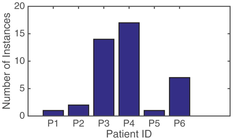
Distribution of baseline shift instances across patient fractions.

1. Leave one patient out—We first execute the leave-one-patient-out analysis using the six patients in the dataset who contributed positive instances of baseline shifts to the dataset. Table 4 shows the test results for patients when they are not included in the training mix, and shows the precision and recall for the baseline shift classification. The negative instances, although not irrelevant, are not considered here since we can have a margin for false positives. Nevertheless, the negative instances are consistently well classified and show high precision and recall values. It is obvious that the holistic performance of any of the classifiers is not optimal when it comes to being tested on a previously unseen patient. However, it is also noteworthy that the patients yielding really low accuracies are those who do not have a substantial presence of positive instances of baseline shifts in their data. The existing distribution is illustrated in figure 4.

   In order to evaluate the sufficiency of this modeling and the results observed, we test the hypothesis that using data from other patients in the dataset (who do not exhibit baseline shifts) would improve prediction performance. Thus the analysis was repeated using all patients in the dataset. The prediction performance of three classifiers in this iteration of the experiment is compared to the previous iteration in terms of F-scores, which is the weighted average (harmonic mean) of the precision and recall (see figure 5). Through, a paired t-test, we observed that the difference in prediction performance is not significant (p > 0.05). This indicates that using data from patients who do not exhibit baseline shifts does not significantly improve the prediction performance of the classification models. However, the significance of these findings could be better demonstrated if a larger dataset of patients exhibiting baseline shifts were available.

2. Train and test on a single patient—Datasets from two patients were chosen in this study based on their contribution of positive baseline shift instances (see figure 4). For each of these patients, the first half of the data provided was used for training the model, while the other half was used for testing. It was ensured that the distribution of baseline shift instances between the training and testing sets were comparable. The results (see table 5) seem to suggest that a single patient’s data is not self-sufficient in knowledge. In other words, it is not enough for a model to simply train on segments of the patient that needs to be tested, and information obtained from other patients may prove useful. This is bolstered by the fact that there is a marked decrease in the classification performance for both positive and negative classes. This may be attributed to the lack of adequate samples for both classes within a single patient.

Table 4.

Comparison of precision and recall (%) for three classification models—Naïve Bayes, linear discriminant and Adaboost. Results correspond to patients that were not included in training set for leave-one-patient-out testing.

Patient	Naïve Bayes		Linear discriminant		Adaboost
	Precision	Recall	Precision	Recall	Precision	Recall
P1	0	0	0	0	0	0
P2	81	50	0	0	0	0
P3	93	79	96	86	98	64
P4	98	94	98	53	0	0
P5	44	100	58	100	94	100
P6	93	100	97	100	0	0

Figure 5.

Comparing F-scores of two classifiers in two iterations of leave-one-patient-out analysis—first with only patients exhibiting baseline shifts, and the second with all patients.

Table 5.

Comparison of precision and recall (%) for two classification models—linear discriminant and Adaboost—for training and testing on the same patient.

Patient	Linear discriminant		Adaboost
	Precision	Recall	Precision	Recall
P3	72	35	0	0
P4	28	58	50	47

4.2.3. Performance evaluation for baseline shift prediction

The ROC curves for three classification models—Naïve Bayes, linear discriminant and Adaboost ensemble—along with the average AUCs are presented in figure 5. To establish the consistency of the comparative performance of the three classifiers, we study the variation of the AUCs for each classifiers for 100 iterations of the 5-fold cross validation. The results for this are presented in figure 6.

Figure 6.

Binary classification performance: ROC curves for three classifiers for 100 iterations of 5-fold cross validation. Mean AUC for linear discriminant = 0.9878; ensemble Adaboost = 0.9794; and Naïve Bayes = 0.9648.

The results indicate that all three classification models show good performance in the binary classification task to predict baseline shifts. The linear discriminant classifier yields the highest robustness and consistency (mean AUC = 0.9878), followed closely by the ensemble Adaboost (mean AUC = 0.9794), and the Naïve Bayes (mean AUC = 0.9648) models.

5. Discussion and conclusion

The objective of this study was to develop techniques that enable us to predict baseline shifts before they occur (an approximate look-ahead window of 5 s) so that radiation dose delivery can be paused either automatically or even potentially through manual intervention by a therapist. The latter is arguably more widely clinically translatable since many smaller centers (which perform the vast majority of radiotherapy procedures) may not have access the latest linac technology with real-time communication with the position monitoring system and realtime gating capabilities.

The trend-based analyses indicate that with some prior knowledge of the patient’s tumor motion trajectories, high accuracies for baseline shift prediction (≈90%) are achievable. The trend-based analysis offers some key preliminary inferences in the utility of predictive modeling using the tumor motion traces. It is observed that while training on information from multiple patients is useful in making the classifiers robust in their performance, such models do not perform well in case of previously unseen patient data. However, once trained with some initial annotated information from a patient’s tumor motion trace (over a duration of 5–10 min), and aided by offline training using prior knowledge from other similar patients, classification models show improvement in incremental baseline trend prediction, including baseline shift occurrences. The prediction latencies do not exceed a few hundred milliseconds, and thus are very conducive to real time applications. An important takeaway is that prediction accuracy decreases with increasing diversity in annotations. Thus, in the interest of accurate baseline shift predictions, it is beneficial to model the problem as one of binary classification. On combining non-baseline occurrences into a single class, a substantial skew is induced in the class distribution, which is compensated by oversampling the weak positive class. Using a revised definition for baseline annotation and skew compensation, binary classification of baseline shifts is significantly improved, with precision and recall values as high as 97% and 88%. The ROC analysis with 5-fold cross validation yields high AUCs between 0.96–0.98. The results of these analyses suggest that predictive algorithms could capitalize on modeling insights obtained from similar patients for accurate predictions in a new patient. Also, including some initial information (5–10 min) from the new patient being treated could help enhance the relevance of the model, thus boosting prediction performance.

While it establishes the utility of predictive modeling of baseline shifts, this study is not without its limitations. The foremost among them is the absence of proper ground truth annotations in the dataset. This issue been addressed here using a heuristic definition for a baseline shift validated by a clinical expert. While this is an acceptable solution for now, future data collection procedures should provide for online tagging of events and significant anomalies upon detection. This would result in a rich and diverse source of information for improved modeling of the tumor motion and enhancing the prediction performance. Secondly, the online analyses in this study are of a simulated nature, achieved by mimicking real world situations by providing data to the classifier in a sequential manner for training and testing. However, prior to its deployment, any such predictive analytical model will have to be tested rigorously in the treatment environment. The performance of the model in such tests would be critical in further validating the utility of the approach in improving treatment and reducing dosage errors.

In this work, two important parameters of the prediction models are the feature window (the 1 min tumor motion segment over which motion features are extracted) and the prediction window (the 5 s tumor motion segment immediately following the feature window). These durations were chosen as reasonable values to evaluate and establish the utility of prediction models. A feature window over a longer duration may capture more information while abstracting (averaging) useful information, whereas a shorter window might to the opposite. Similarly, shorter prediction windows may not be able to capture gradual baseline shifts occurring over longer durations. While beyond our current scope, we believe that for clinical translation of this approach, it would be valuable and, arguably, necessary to evaluate the prediction performance for different lengths of the feature and prediction windows.

The impact of this study is not restricted to prediction of baseline shifts or motion anomalies. The significance of these analyses extends to the domain of personalized treatment through patient similarity. The trade-off between the prior knowledge obtained from patients and the new information from a new patient forms the basis for optimized learning. Identifying subgroups among the patient population on the basis of common characteristics exhibited by members can help in profiling a future patient and choosing a treatment plan that would be most optimal. Moreover, with the provision of handling transitions among different behavior types, future motion management approaches can improve the treatment efficacy by modifying it to the patient’s evolving characteristics over time.

References

- Adler J, Chang S, Murphy M, Doty J, Geis P, Hancock S. The cyberknife: a frameless robotic system for radiosurgery. Stereotactic Funct Neurosurg. 1997;69:124–8. doi: 10.1159/000099863. [DOI] [PubMed] [Google Scholar]
- Arlot S, Celisse A. A survey of cross-validation procedures for model selection. Stat Surv. 2010;4:40–79. [Google Scholar]
- Batal I, Valizadegan H, Cooper GF, Hauskrecht M. A pattern mining approach for classifying multivariate temporal data. Proc IEEE Int Conf Bioinformatics and Biomedicine. 2011:358–65. doi: 10.1109/BIBM.2011.39. [DOI] [PMC free article] [PubMed] [Google Scholar]
- Brown C, Davis H. Receiver operating characteristics curves and related decision measures: a tutorial. Chemometr Intell Lab Syst. 2006;80:24–38. [Google Scholar]
- Cover TM, Hart PE. Nearest neighbor pattern classification. IEEE Trans Inf Theory. 1967;13:21–7. [Google Scholar]
- Domingos P, Pazzani M. On the optimality of the simple Bayesian classifier under zero-one loss. Mach Learn. 1997;29:103–30. [Google Scholar]
- Fawcett T. An introduction to ROC analysis. Pattern Recognit Lett. 2006;27:861–74. [Google Scholar]
- Fisher R. The use of multiple measurements in taxonomic problems. Ann Eugenics. 1936;7:179–88. [Google Scholar]
- George R, Suh Y, Murphy M, Williamson J, Weiss E, Keall P. On the accuracy of a moving average algorithm for target tracking during radiation therapy treatment delivery. Med Phys. 2008;35:2356–65. doi: 10.1118/1.2921131. [DOI] [PMC free article] [PubMed] [Google Scholar]
- Hastie TJ, Tibshirani RJ, Friedman JH. The Elements of Statistical Learning. New York: Springer; 2009. [DOI] [Google Scholar]
- Keall P, et al. The management of respiratory motion in radiation oncology report of AAPM task group 76. Med Phys. 2006;33:3874–900. doi: 10.1118/1.2349696. [DOI] [PubMed] [Google Scholar]
- Lee SJ, Motai Y. Review: Prediction of Respiratory Motion. Berlin: Springer; 2014. pp. 7–37. [Google Scholar]
- Pepin E, Wu H, Shirato H. Dynamic gating window for compensation of baseline shift in respiratory-gated radiation therapy. Med Phys. 2011;38:1912–8. doi: 10.1118/1.3556588. [DOI] [PMC free article] [PubMed] [Google Scholar]
- Ruan D, Fessler JA, Balter JM. Real-time prediction of respiratory motion based on local regression methods. Phys Med Biol. 2007;52:7137–52. doi: 10.1088/0031-9155/52/23/024. [DOI] [PubMed] [Google Scholar]
- Schapire RE. A brief introduction to boosting. Proc. of the 16th Int. Joint Conf. on Artificial Intelligence; San Francisco, CA: Morgan Kaufmann; 1999. pp. 1401–6. [Google Scholar]
- Seiffert C, Khoshgoftaar TM, Van Hulse J, Napolitano A. Rusboost: a hybrid approach to alleviating class imbalance. IEEE Trans Syst Man Cybern A. 2010;40:185–97. [Google Scholar]
- Seppenwoolde Y, Berbeco R, Nishioka S, Shirato H, Heijmen B. Accuracy of tumor motion compensation algorithm from a robotic respiratory tracking system: a simulation study. Med Phys. 2007;34:2774–84. doi: 10.1118/1.2739811. [DOI] [PubMed] [Google Scholar]
- Suh Y, Dieterich S, Cho B, Keall P. An analysis of thoracic and abdominal tumour motion for stereotactic body radiotherapy patients. Phys Med Biol. 2008;53:3623–40. doi: 10.1088/0031-9155/53/13/016. [DOI] [PubMed] [Google Scholar]
- Tachibana H, Kitamura N, Ito Y, Kawai D, Nakajima M, Tsuda A, Shiizuka H. Management of the baseline shift using a new and simple method for respiratory-gated radiation therapy: detectability and effectiveness of a flexible monitoring system. Med Phys. 2011;38:3971–80. doi: 10.1118/1.3598434. [DOI] [PubMed] [Google Scholar]
- Vedam S. Respiratory Motion Prediction in Radiation Therapy. Berlin: Springer; 2013. pp. 285–96. [Google Scholar]
- Verma P, Wu H, Langer M, Das I, Sandison G. Survey: real-time tumor motion prediction for image-guided radiation treatment. Comput Sci Eng. 2011;13:24–35. [Google Scholar]
- Wilbert J, et al. Tumor tracking and motion compensation with an adaptive tumor tracking system (ATTS): system description and prototype testing. Med Phys. 2008;35:3911–21. doi: 10.1118/1.2964090. [DOI] [PubMed] [Google Scholar]
- Yoon J, Sawant A, Suh Y, Cho B, Suh T, Keall P. Experimental investigation of a moving averaging algorithm for motion perpendicular to the leaf travel direction in dynamic MLC target tracking. Med Phys. 2011;38:3924–31. doi: 10.1118/1.3590384. [DOI] [PMC free article] [PubMed] [Google Scholar]