Visual threat assessment and reticulospinal encoding of calibrated responses in larval zebrafish

Summary

All visual animals must decide whether approaching objects are a threat. Our current understanding of this process has identified a proximity-based mechanism where an evasive maneuver is triggered when a looming stimulus passes a subtended visual angle threshold. However, some escape strategies are more costly than others and so it would be beneficial to additionally encode the level of threat conveyed by the predator's approach rate to select the most appropriate response. Here, using naturalistic rates of looming visual stimuli while simultaneously monitoring escape behavior and the recruitment of multiple reticulospinal neurons, we find that larval zebrafish do indeed perform a calibrated assessment of threat. While all fish generate evasive maneuvers at the same subtended visual angle, lower approach rates evoke slower, more kinematically variable escape responses with relatively long latencies as well as the unilateral recruitment of ventral spinal projecting nuclei (vSPNs) implicated in turning. In contrast, higher approach rates evoke faster, more kinematically stereotyped responses with relatively short latencies, as well as bilateral recruitment of vSPNs and unilateral recruitment of giant fiber neurons in fish and amphibians called Mauthner cells. In addition to the higher proportion of more costly, shorter latency Mauthner-active responses to greater perceived threats, we observe a higher incidence of freezing behavior at higher approach rates. Our results provide a new framework to understand how behavioral flexibility is grounded in the appropriate balancing of trade-offs between fast and slow movements when deciding to respond to a visually perceived threat.

Introduction

When an animal perceives an oncoming predator, it is critical to correctly choose whether, when, and how to move to survive the impending attack. Looming visual stimuli, simulating an approaching predator, provide an opportunity to investigate the underlying mechanism of threat assessment involved in this set of decisions [1, 2]. The current consensus across a variety of vertebrate and invertebrate organisms is that an approaching predator triggers a ballistic escape response once it reaches a certain subtended angle threshold [3, 4, 5, 6]. Given the constraints on predator size, this angle threshold is equivalent to a proximity threshold.

Within vertebrates, this theory of a proximity-based response aligns well with findings from a bilateral pair of giant fiber interneurons in the brainstem of fish, called Mauthner cells [7]. Mauthner cells collect sensory information from one side of the body and transmit it to the other side via a large caliber axon [8, 9], resulting in a strong contraction of body muscles opposite to the stimulus that generates a short-latency evasive turn. Mauthner cells respond to visual, tactile, vestibular, auditory, lateral-line and electric field stimuli [10, 11, 12, 13, 14, 15] and are difficult to excite [16, 17, 18]. The conclusion from these studies across various modalities is that the decision to escape is a result of reaching the Mauthner cell firing threshold due to strong sensory input, as would arise from an approaching predator that has traversed the proximity threshold.

However, with a proximity mechanism there is no way to distinguish between an object that passes the proximity threshold rapidly versus slowly, corresponding to threats of differing urgency. Moreover, while Mauthner cells expedite signal propagation and ensure quick reflexes, the power and relatively stereotyped reactions they produce can exact energetic costs and be exploited by predators [19, 20, 21]. It would therefore be beneficial to encode speed of approach as an additional means to decide whether to engage the giant fiber escape systems or alternate, less costly strategies, such as no response or a less rapid, more flexible response. Currently it is unknown whether vertebrates use approach rate to inform the trade-off between short-latency, ballistic movements and long-latency, more variable movements.

Here, we test the hypothesis that approach rate modulates escape behavior in larval zebrafish by using virtual looming stimuli with naturalistic sizes and approach rates, high-speed kinematic analysis in free swimming animals, and in vivo calcium imaging in partially restrained ones to assess the contribution of Mauthner cells to the observed behavior. While zebrafish larvae did evade looming stimuli at a fixed subtended angle and distance as expected from prior work, markedly different behaviors occurred as a function of approach rate. Lower approach rates evoked a more kinematically variable escape response with longer latency, and recruitment of ventral spinal projecting nuclei (vSPN) implicated in turning responses [22] but not activation of the Mauthner cells. Faster approach rates produced more kinematically stereotyped responses with shorter latency that did involve Mauthner cell activation in addition to more robust recruitment of vSPNs. We also observe evidence for freezing behavior, which is more likely to occur in response to rapidly approaching stimuli.

Collectively, our findings support a calibrated assessment of threat based on approach rate in addition to the previously described threshold based on the subtended angle of the approaching object. In this threat assessment logic, the approach rate (proportional to threat urgency) sets the probability of movement, its latency, speed, and variability, while the subtended angle threshold determines the timing of the movement. We discuss the implications of our findings for the neural processing of threat, how threat level is conveyed to the motor system, and the evolution of escape behavior.

Results

Timing and kinematics of looming evoked responses

Larval fish (3.5–5 mm) at 5–7 days post fertilization (dpf) were placed in a smaller dish within a larger dish (Figure 1A) and shown looming stimuli projected onto diffusive paper around the edges of the larger dish. The virtual looming stimulus was a black square expanding on a blue background of stationary, low contrast rectangles (Figure 1B₂).

Figure 1. Timing and kinematics of looming evoked responses.

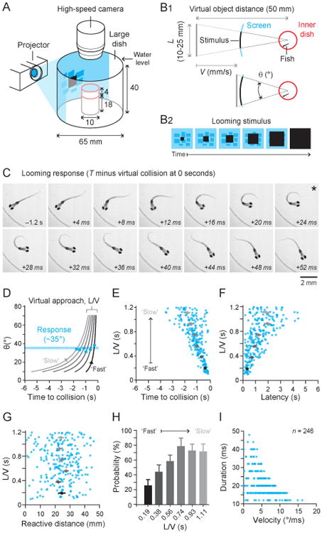
A) Larval zebrafish (N_fish = 21) were contained in a smaller covered chamber (shown in red) fully submerged in a larger dish filled with water. Responses were recorded with high speed videography at 250 fps from above. B₁) Virtual looming stimuli were defined by L, the size of the square, V, the velocity, and the apparent distance covered by the object (50 mm in this study). The time-varying subtended angle θ is determined by the parameter L/V. The azimuth of the stimulus with respect to the fish's head depends on the orientation of the fish, and therefore ranged from ±180°, with left being negative and right being positive. B₂) The stimulus was a black square expanding over time on a stationary blue background of low contrast rectangles. C) A representative looming evoked response with the time of response defined by time being negative before virtual collision at 0 seconds. This response is typical in that the largest directional change happened by the end of the initial bend—marked with asterisk—followed by undulatory swimming. D) Fish respond at a specific subtended angle of the looming object regardless of looming rate. We binned time of responses according to particular constant values of L/V (Bin 1: center L/V = 0.19 s, N_trials = 29, Bin 2: center L/V = 0.38 s, N_trials = 34, Bin 3: center L/V = 0.56 s, N_trials = 45, Bin 4: center L/V = 0.74 s, N_trials = 49, Bin 5: center L/V = 0.93 s, N_trials = 44, Bin 6: center L/V = 1.11 s, N_trials = 44), corresponding to specific curves of θ versus time. The curve drawn with the darkest line represents the smallest L/V bin center—a fast looming stimulus—and the lightest curve represents the largest L/V bin center—a slow looming stimulus. By marking the mean response time relative to time of virtual collision for each group (blue dots), we find that fish responded on average when θ = 35° ± 15° (std, N_trials = 246). E) The average onset time of the looming evoked response (mean ± SEM in gray) increased with increasing L/V as found with other model animals, with larger L/V s having more variable response times. F) The response latency from stimulus onset (mean ± SEM in gray) and the variability of the latency also increased with increasing L/V. G) The virtual distance (mean ± SEM in gray) from the looming stimulus at the time of fish response did not change with L/V. H) Fish (N_fish = 21) were more likely to respond to slow looming stimuli (higher L/V s) than fast looming stimuli (low L/V s). I) Fish manipulated both the duration of the initial bend and the yaw velocity of the initial bend to control the total head yaw achieved by the end of the initial bend. Horizontal bands are due to the 4 ms interval between video frames. See also Figure S1 and S2.

The looming stimulus (Figure 1B) is defined by the size of the approaching object of equal width and height (L), the approach velocity (V), and the apparent distance covered (d), with the subtended angle θ to the snout (with respect to head orientation) being determined by these parameters (Figure 1B₁). The combined term L/V is an indicator of the expansion of θ with time and is used as a stimulus parameter as it allows comparison to looming-evoked responses in other animals quantified with the same parameter [2, 23]. The L/V term was psuedorandomly selected with uniform probability between 0.1–1.2 seconds (s), since prior studies have shown this to be naturalistic [24]. L was psuedorandomly selected with uniform probability between 10–25 mm (also naturalistic: [24]), with the apparent starting distance of the stimulus d held constant at 50 mm. The relative azimuthal angle of the stimulus depended on the freely swimming fish orientation, but varied between ±180° (left negative, right positive) and sampling was verified to be uniform (Figure S1).

High speed videography at 250 frames-per-second (fps) was used to record the looming-evoked response from above. Figure 1C depicts a representative looming evoked response to a looming stimulus with L/V = 0.4 s and azimuth 43°. The response starts at −1.2 s since time is negative before the virtual collision at 0 s. During the looming evoked response, the fish re-oriented with an initial bend (Figure 1C, end of initial bend marked with asterisk) and swam away with undulatory swimming during a propulsive stage.

Figure 1D plots 6 curves of different expansions of θ with time which correspond to 6 different values of L/V. These 6 L/V values are the centers of 6 equally-spaced bins in the range of L/V s tested (0.1–1.2 s) in this study. The average response time for each bin is plotted on the curves describing the expansion of θ with time. We found that the fish respond at approximately θ = 35° (Figure 1D), for different values of L/V. The dashed line is the average θ (35° ± 15°, μ;±std) at the time of response for all recorded responses for the continuum of L/V s tested. The similarity between the population average and the average of each bin demonstrates that the average θ at the time of response deviated little for different L/V s or looming rates, as has been recorded for looming evoked responses from other animals [3, 23, 2, 25].

The existence of this critical subtended angle influenced both the timing of the fish response and the apparent distance from the virtual object when the fish responded. The length of time to collision from the onset of the fish's response increased with increasing L/V (Figure 1E), also found to be true for larval zebrafish by other researchers [6, 26]. The response latency increased with increasing L/V (Figure 1F). However, the mean reactive distance—the apparent distance from the virtual object at the time of fish response—did not change with L/V, suggesting the existence of a critical reactive distance of ∼25 mm.

While Figure 1D and G indicate that the fish were performing looming evoked responses at some angular or distance threshold, Figure 1H shows that fish were much more likely to respond to larger L/V s—slow looming stimuli—than smaller ones—fast stimuli, demonstrating that response probability is modulated by the approach rate of the stimulus. We found that fish used the duration of the initial bend and the head yaw velocity during the initial bend to produce different total changes in orientation for all of recorded responses (Figure 1I).

Directionality of looming evoked responses

An analysis of the kinematics of each looming evoked response was performed to investigate their relationship to the approach rate of the stimulus. In order to quantify the escape trajectory, we measured the initial bend angle for all responses and the final heading angle (both defined in Figure 2A) for a subset of responses where the trajectory of the response was not obstructed by the wall of the smaller dish. Figure 2B shows that the initial bend angle was a good predictor of the final heading angle. Therefore, the initial bend angle was used as an indirect measure of the final heading angle. Changes in elevation were not measured since the dish was only 4 mm deep (Figure 1A).

Figure 2. Directionality of looming evoked responses.

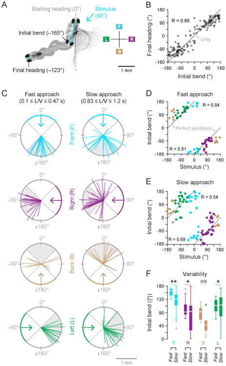
A) The initial bend angle was measured for all responses (N_fish = 21, N_trials = 246) and the final heading angle was measured for a subset of responses (N_fish = 21, N_trials = 149) where the looming evoked response was not obstructed by the wall of the smaller dish. B) The initial bend angle was a strong predictor of the final heading angle and largely determined the escape direction, as evidenced by R = 0.95. C) The direction and translation of the head after the initial bend of responses were grouped by fast (small L/V s) or slow looming (large L/V s) stimuli and by the quadrant of the looming stimulus azimuth Front (−45° −45°], Right (45° – 135°], Back (135° – 180° and −180° – −135°], and Left (−135° – −45°]. Responses showed stimulus dependent response patterns – Front-fast looming: N_trials = 19, Front-slow looming: 22, Right-fast: 18, Right-slow: 32, Back-fast: 12, Back-slow: 16, Left-fast: 16, Left-slow: 22. D) The stimulus azimuth and the initial bend angle for fast looming stimuli (N_trials = 65) were highly correlated with the lines of ‘perfect avoidance’ which correspond to a turn which directs the fish exactly 180° away from the stimulus. E) The stimulus azimuth and the initial bend angle for slow looming stimuli (N_trials = 92) were modestly correlated with the lines of ‘perfect avoidance’ due to increased variance. F) The boxplots of the absolute value of the initial bend angle for responses grouped according to azimuthal angle of the stimulus and slow or fast stimuli show a significant increase in variability of the initial bend angle when fast and slow looming stimuli were compared. This was true within each quadrant of looming stimulus azimuth, except for stimuli approaching from the back (Levene's test, Front: N_{trials, fast} = 19, N_{trials, slow} = 22, p = 0.007, Right: N_fast = 18, N_slow = 32, p = 0.011, Back: N_fast = 12, N_slow = 16, p = 0.372, Left: N_fast = 16, N_slow = 22, p = 0.021). The absolute value of the initial bend angle was used to compute statistical significance of the variance since the discontinuity between +180° and −180° could introduce erroneously large values for variance. Bottom and top of each box indicate the 25th and 75th percentiles, respectively; white line is median, whiskers extend to the last point that is not an outlier (an outlier is defined as more than 1.5 times the interquartile range beyond the median). Asterisks signify the p-value range for statistical tests. * 0.01 < p ≤ 0.05, ** 0.001 < p ≤ 0.01, *** p ≤ 0.0001.

Figure 2C shows the vector from the center of the eyes in the starting frame to the center of the eyes at the end of the initial bend across different stimulus directions. These are grouped by small L/V s—fast approach—and large L/V s—slow approach. The boundaries for the small and large L/V groups were determined by using the smallest one-third and the largest one-third of the range of L/V s tested in this study (responses to middle third are not shown for clarity). Directionality differences in the initial bend between fast and slow stimuli are immediately evident.

Figure 2D shows the initial bend angles of responses to fast looming stimuli plotted against the azimuthal angle of the stimulus. The initial bend angles to fast approaches were highly correlated with lines of ‘perfect avoidance’ – a turn which directs the fish's head 180° away from the stimulus. The initial bend angles to slow looming stimuli were modestly correlated with ‘perfect avoidance’ which indicates that the fish still tended to head away from the approaching stimulus but with increased variability (Figure 2E).

Figure 2F demonstrates that there was a significant increase in the variability of the absolute initial bend angle when comparing responses to fast looming stimuli with those to slow looming stimuli, except for cases where the stimuli approached from the back. The results in Figure 2F indicate that that the variability in the direction of evasive response involves an assessment of the approach rate of the threat.

Tail kinematics of partially restrained looming evoked responses

Further experiments were performed in a partially restrained preparation (Figure 3A) since it permitted strict control over the environment, made detailed automated tracking of tail kinematics during the initial bend possible, and enabled calcium imaging at single neuron resolution during behavior.

Figure 3. Tail kinematics of partially restrained looming evoked responses.

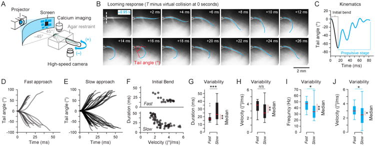
A) Fish (N_fish = 18) were partially-restrained in agar with their tails free to move and positioned to view virtual looming stimuli projected onto a screen and approaching from the front. High speed videography was used to record tail movement at 1000 fps. B) The entire tail was tracked and the tail angle was computed for all responses to quantify the looming evoked response. The agar restraint stopped at the end of the swim bladder marked with a dashed white line. C) Tail kinematics during the initial bend (in black) and the propulsive stage (in cyan) were extracted from the responses. D) The progression of the tail angle during the initial bend grouped by responses to fast stimuli (small L/V s, N_trials = 25) and E) slow stimuli (large L/V s, N_trials = 63) showed qualitative differences. F) Fish controlled absolute tail angle velocity and initial bend duration differently under each stimulus paradigm. The absolute value was used to group right and left turns together as was done in the free swimming case. G) Responses to fast stimuli had a shorter median (Mann-Whitney U test, p = 0.005) and less variable (Levene's test, p < 0.001) initial bend duration but H) a faster (Mann-Whitney U test, p = 0.002) and non-significantly different tail angle velocity (Levene's test, p = 0.177) when compared to responses to slow stimuli. I) Responses to fast stimuli also had a higher (Mann-Whitney U test, p = 0.002) and less variable (Levene's test, p = 0.034) frequency of swimming with J) higher (Mann-Whitney U test, p = 0.021) and less variable (Levene's test, p = 0.032) average absolute tail angle velocities during the propulsive stage. See also Figure S3 and S4.

Individual larvae at 5–7 dpf were partially restrained in agarose (Figure 3A) and positioned to view looming stimulus projections on a diffusive screen. Looming stimuli were psuedorandomly selected from the same range of L/V s used previously but the azimuthal angle of the stimulus varied uniformly between −45° and +45°. Stimuli were restricted within this azimuthal range since responses to stimuli approaching from the front provided the highest confidence (smallest p-value) in their being a difference between responses to fast and slow stimuli (Figure 2F). High speed videography at 1000 fps was used to capture body movements through a 4× objective below the transparent dish in which the fish was placed. The shape of the body from the caudal swim bladder to the end of the tail was tracked with a custom Matlab program (Figure 3B). The tail angle, which is the angle between the heading vector and a vector from the caudal edge of the swim bladder to the end of the tail (Figure 3B), was quantified over the course of a swim bout (Figure 3C). The initial bend is easily identified (drawn in black, Figure 3C) in the progression of the tail angle over time during the first unilateral contraction of the tail with the propulsive stage (drawn in cyan, Figure 3C) directly following.

Figures 3D and E show the tail angle for all recorded responses during the initial bend grouped by fast and slow stimuli where the same L/V boundaries as in the free swimming experiments were used for grouping. The differences of the tail angles between the two groups visible in Figures 3D and E is quantified in Figure 3F. This shows that the fish controlled the duration of the initial bend and the absolute average tail angle velocity during the initial bend differently across stimulus paradigms. The initial bend duration and the tail angle velocity together allow for inferences about the initial bend angle because the tail angle velocity of free swimming fish were strongly correlated with the head yaw velocity during the initial bend (Figure S4).

The data in Figure 3F is further analyzed in Figures 3G and H which demonstrate that the responses to slow stimuli had initial bend durations which were significantly longer and more variable than those to fast stimuli. Moreover, the absolute tail angle velocities of responses to slow stimuli were lower but had a non-significant difference in variability from responses to fast stimuli. The results in Figure 3G and H together show that the looming-evoked response kinematics vary with L/V and the increase in variability of the duration is the largest contributor to variability in the initial bend.

Although both fast and slow stimuli had on average 3 tail cycles in the propulsive stage (Figure 3C) there were significant differences in the kinematics during the propulsive stage for the two stimulus paradigms (Figure 3I and J). Responses to slow stimuli had average tail cycle frequencies (Figure 3I) in the propulsive stage which were lower and more variable. Additionally, the average absolute tail angle velocity of responses to slow stimuli during the propulsive stage was lower and more variable.

Mauthner cell activity to varying approach rates

A previously established protocol was used to backfill the reticulospinal network neurons of larval zebrafish with Calcium Green dextran [27] before being shown looming stimuli at 5–7 dpf. In the partially restrained looming stimulus assay, we simultaneously measured neural activity in the M-cell from above with a 40× objective and body kinematics from below with a 4× objective (Figure 3A). Fish were shown a fixed slow stimulus (L/V = 1.0 s) and a fast stimulus (L/V = 0.4 s), both at an azimuth of 30° from the left (Figure 4A). Only two fixed approach rates were used rather than the full set because surveying the full set of approach rates was impractical.

Figure 4. Mauthner cell activity to varying approach rates.

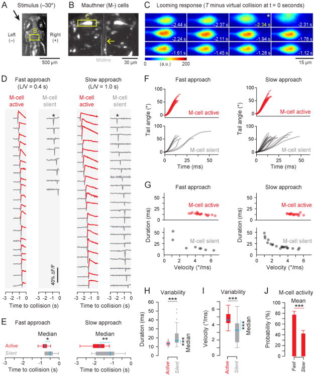
A) Partially restrained fish (N_fish = 15) were shown a fast (L = 11 mm, L/V = 0.4 s, d = 50 mm) and a slow (L = 11 mm, L/V = 1.0 s, d = 50 mm) looming stimulus at an azimuth of −30°, which consistently produced rightward looming evoked turns. B) The M-cell (within yellow square) is in the larval zebrafish hindbrain with contralateral axonal projections known to mediate rightward turns. Calcium imaging of the left M-cell was performed in all fish at 30 fps. High speed videography of the tail movement was simultaneously performed at 1000 fps. C) A representative M-cell active response with the frame corresponding to the start of the looming evoked response marked with a star and a motion artifact immediately following. This montage demonstrates the increase in fluorescence during neuronal activity and the quality of signals acquired with the imaging assay. D) Calcium imaging fluorescence traces for all responses ordered by response time and grouped by fast looming M-cell active (N_trials = 19) and silent (N_trials = 8) or slow looming M-cell active (N_trials = 19) and silent (N_trials = 21). M-cell activity was determined by a threshold of ΔF/F = 5%. E) In both stimulus paradigms, M-cell active responses occurred significantly earlier (more negative time, Mann-Whitney U test, p < 0.01 for both cases) than M-cell silent responses with mean ± std as follows: Fast_{M-cell active}: −0.80 ± 0.17 s, Fast_{M-cell silent}: −0.52 ± 0.27 s, Slow_{M-cell active}: −1.80 ± 0.44 s, Slow_{M-cell silent}: −1.27 ± 0.59 s. F) The progression of the tail angle during the initial bend of responses to fast and slow stimuli grouped by M-cell active or silent showed immediate differences. G) M-cell active responses under different stimuli had similar initial bend durations and tail angle velocities but were different from M-cell silent responses. H) M-cell active responses had a shorter (Mann-Whitney U test, p ≪ 0.001) and less variable (Levene's test, p ≪ 0.001) distribution of initial bend durations than M-cell silent responses. I) M-cell active responses had a higher (Mann-Whitney U test, p < 0.001) and less variable (Levene's test, p < 0.001) distribution of tail angle velocities during the initial bend than M-cell silent responses. J) Fish (Nfish = 15) were much more likely to produce an M-cell active response to a fast stimulus than to a slow stimulus (Student's t test, p < 0.001). See also Figure S5.

Figure 4B shows a representative maximum-intensity z-projection fluorescent image of a portion of the reticulospinal network with the left M-cell inscribed within a yellow rectangle. The left M-cell has one commissural axon which is known to mediate escape turns to the right [28]. Since z-stacking was too slow in this case for neural activity imaging during behavior, the M-cell was imaged at 30 fps in a single plane in a small region that just encompassed the neuron (Figure 4C).

Figure 4C shows a montage of fluorescence images from a single trial where the fish performed an M-cell active looming evoked response. The looming evoked response occurs at −2.34 s and is immediately followed by a motion artifact in the imaging due to the vigorous nature of the aversive response. This is followed by increased flourescence due to neural activity.

Figure 4D shows all of the fluorescence traces from all recorded responses grouped by the speed of stimuli. Fluorescence traces from the M-cells of fish performing looming evoked responses were compiled into M-cell active and silent groups based on a decision threshold at ΔF/F = 5% (Figure S5). All fluorescence traces show a sharp drop at the time of response due to the motion artifact (Figure 4C) in fluorescence imaging.

M-cell active responses happened significantly earlier (more negative response times) than M-cell silent responses for both fast (284 ms difference in medians) and slow (563 ms difference in medians) stimuli (Figure 4E). The tail angle during the initial bend of M-cell active and silent responses grouped by the fast and slow stimuli also showed differences (Figure 4F). These differences are further quantified in Figure 4G which demonstrate that the M-cell active responses had different initial bend durations and tail angle velocities from M-cell silent responses for the both fast and slow looming stimuli. Figure 4H shows that the initial bend duration for M-cell active responses were significantly smaller and less variable than M-cell silent responses. The tail angle velocity during the initial bend for M-cell active responses was also significantly higher (Figure 4I) and less variable than M-cell silent responses. There was difficulty in tracking propulsive stage parameters for all responses as some fish started struggling during the propulsive stage, probably due to the partial restraint. However, for the subset of tracked responses, propulsive stage frequency and tail angle velocity were less variable for M-cell active responses (Levene's test, N_{M-cell active} = 28, N_{M-cell silent} = 21, p < 0.001). The proportion of M-cell active responses is far higher for fast stimuli than for slow stimuli (Figure 4J).

Reticulospinal recruitment during Mauthner active and silent responses

To study recruitment differences in the reticulospinal network between Mauthner cell active and silent looming-evoked responses, volumetric calcium imaging was performed on a subset of the reticulospinal neurons in conjunction with high-speed behavior imaging while larval zebrafish responded to the same fast or slow looming stimuli described above. Light field microscopy was used to acquire volumetric calcium fluorescence data (70 μm × 100 μm × 100 μm) at 15 fps from the Mauthner cells (M-cells) and its homologs, MiD2 and MiD3, along with other ventral spinal projecting neurons (vSPNs) that have been identified in previous literature to be involved in turning behavior [22]. These vSPNs include RoV3, MiR1, MiM1, MiV1, MiR2, and MiV2, listed here in rostrocaudal order of anatomical occurrence (as they appear in the top panel of Figure 5A).

Figure 5. Reticulospinal recruitment during Mauthner cell active and silent responses.

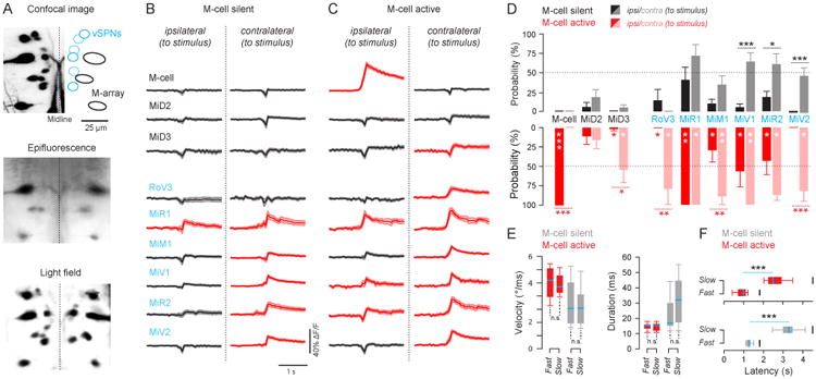
A) Compares the maximum intensity z-projection of a volume acquired with confocal microscopy (top, acquisition time: 10 mins) with a single plane from epifluorescence microscopy within the same volume (middle, acquisition time: 50 ms) and a max intensity z-projection of the same volume reconstructed from a light field image (bottom, acquisition time: 50 ms) demonstrating the utility of light field imaging as a fast volumetric imaging system able to resolve the neurons of interest. In this study, we specifically focused on the Mauthner cell and its homologs (M-array, top, in black) along with the ventral spinal projecting neurons (vSPNs, top, in blue). B) Plots show the average calcium signals with upper and lower SEM boundaries from each nucleus during M-cell silent looming-evoked responses across all trials (25 ≤ N_trials ≤ 35, for exact values see tables in STAR Methods) and C) The same is shown for M-cell active looming evoked responses (34 ≤ N_trials ≤ 50). Nuclei names are color-coded in black or blue in accordance with their membership in either the M-array or the vSPNs. Red traces denote nuclei for which the mean of the calcium signal reached above the ΔF/F threshold (5%) for activation. D) Shows the average ±SEM recruitment probability of nuclei for M-cell active and silent cases grouped by fish (5 ≤ N_fish ≤ 17, Student's two-tailed t-test). E) Demonstrates the similarity of angular velocity and bend duration distributions within M-cell active and M-cell silent cases regardless of approach rate (M-cell active: N_Fast = 24, N_Slow = 26, M-cell silent: N_fast = 11, N_Slow = 24). F) Shows the differences in latency of M-cell active and M-cell silent responses from the onset of the stimulus for each approach rate (Mann-Whitney U test, p < 0.001). The latency of the responses from stimulus onset are the following: M-cell Active_fast: 0.99 ± 0.17 s, M-cell Active_slow: 2.47 ± 0.38 s, M-cell Silent_fast: 1.3 ± 0.25, M-cell Silent_slow: 3.31 ± 0.51. Short black bars at 1.82 s and 4.54 s mark the latency at which each stimulus would collide with the fish. See also Figure S6.

Light field imaging was ∼10,000 times faster than confocal imaging (confocal image example Figure 5A top) for acquiring the volume of interest. A standard epifluorescence image at a single plane (Figure 5A, middle) is insufficient to reconstruct the entire volume. However, a modified epifluorescence scope with a microlens array provides a light field with sufficient information to reconstruct the volume (Figure 5A, bottom)[29]. After post-processing, segmenting, and anatomically labeling volumes reconstructed from light field microscopy (Figure S6), time-varying calcium signals were extracted from volumes acquired during looming-evoked escapes and grouped into M-cell silent or M-cell active response categories. The signals from these bilaterally symmetric nuclei were also grouped according to their relative location to the stimulus, either on the same side as the stimulus (ipsilateral), or on the opposite side of the stimulus (contralateral). All turns from looming stimuli were away from the stimulus direction; thus the contralateral nuclei are on the same side that the fish turns toward.

The average calcium signals from all trials for each nucleus (Figure 5B and C) show immediate differences in recruitment between M-cell active and silent responses. Red traces denote nuclei for which the mean of the calcium signal reached above the ΔF/F threshold (5%) for activation. These recruitment patterns are further explored in Figure 5D which plots the average probability ± SEM of recruitment grouped by fish for each of the reticulospinal nuclei investigated. The statistical results demonstrate significant differences in the mean recruitment probability between bilaterally symmetric nuclei pairs within and across M-cell active and silent responses.

The MiD3 Mauthner homolog and the RoV3 nuclei contralateral to the stimulus were frequently recruited (MiD3: 55 ± 15% recruitment probability, RoV3: 77 ± 18% recruitment probability) during M-cell active responses but were rarely active during M-cell silent ones. Other nuclei such as MiV1, MiR2, and MiM1 showed prominent changes in the symmetry of bilateral recruitment. While the M-cell silent responses had significant recruitment of MiV1 and MiR2 nuclei contralateral to the stimulus (Figure 5B and D, pMiV1 = 0.0006, pMiR2 = 0.023), M-cell active responses had bilateral recruitment of both nuclei (Figure 5C and D). However, M-cell active responses had significant unilateral recruitment of the MiM1 nuclei contralateral to the stimulus (p = 0.003) while M-cell silent responses show a reduced recruitment of MiM1 nuclei and no significant difference in recruitment of the corresponding ipsilateral MiM1. Some nuclei, like MiR1 and MiV2 have an overall drop in recruitment probability when comparing M-cell silent to active but no changes in symmetry or asymmetry of activation with respect to the corresponding nuclei across the midline.

Figure 5E demonstrates that angular velocity and bend duration distributions of Stage 1 were not significantly different within M-cell active responses for each approach rate or within M-cell silent responses for each approach rate. Despite the similarity of kinematics of M-cell active responses across both stimuli and M-cell silent responses across both stimuli, there are significant differences in the latency from stimulus onset of the responses ranging from 1.5–2.5 s between the two approach rates (Figure 5F).

Discussion

Our goal here was to evaluate how larval zebrafish assess the threat of looming predators to determine the utility of short latency, ballistic responses over longer latency, more variable and less energetically costly behaviors. While previous literature suggested a proximity mechanism of threat assessment [3, 4, 5, 6] which is insensitive to varying levels of threat, we found that fish perform a graded assessment of threat where the approach rate of the looming stimulus modifies the likelihood of an evasive maneuver, its kinematics, and the proportion of Mauthner-mediated evasive responses (Figure 6). Mauthner cell recruitment is more often reserved for urgent threats as it was more likely to occur in response to faster looming stimuli (Figure 6). Slower looming stimuli were less likely to recruit the Mauthner cells and involve escapes which are more delayed and more variable in their kinematics than Mauthner-active escapes (Figure 6). The behavioral utility of more variability in response to slowly approaching objects is supported by modeling studies, which suggest that slower predators allow for a wider range of escape directions that maximize distance [35]. In addition, more variable escape trajectories are arguably less predictable, which would be advantageous when responding to slower and therefore more maneuverable predators [36, 37].

Figure 6. The looming-evoked response is modulated by the approach rate of the looming stimulus.

As a predator nears the critical subtended angle threshold, fish decide to either move or freeze in a probabilistic manner based on the approach rate. If the fish moves, it must decide between Mauthner active and Mauthner silent responses—the probability of which is also determined by the approach rate. Mauthner active and Mauthner silent circuitry have different neural recruitment patterns and produce kinematically distinct behaviors. Mauthner active responses recruit the Mauthner cell along with Mauthner homologs, and other ventral spinal projection neurons to produce a short latency, more stereotyped maneuver, which is generally directed 180° away from the stimulus approach direction (in black). Meanwhile, Mauthner silent responses almost exclusively recruit the ventral spinal projecting neurons to produce longer latency responses with more variable kinematics and escape directions (in blue).

While there are clear differences in the timing and variability of escape turns to slow and fast looming stimuli, almost all responses were evasive in that zebrafish move directly away from the perceived threat. This necessitates a means of directional coding [38]. Our work suggests variations in escape trajectory can be explained largely by the duration of the initial bend, and to a lesser extent by tail angle velocity. This observation is congruent with studies in the spinal cord that have revealed a mechanism of turn angle encoding through modulating the number of spikes in participating excitatory premotor interneurons and motor neurons [39]. Such a mechanism could manipulate changes in duration by modulating firing rate of the interneurons and motor neurons. Given that Mauthner cells typically fire only once during the initial bend [7], the modulation of spike rate and bend duration necessary for direction control must arise elsewhere. The most likely sources for modulation of spike rate and bend duration are other identified reticulospinal neurons, which have been implicated in directional coding of more abrupt sensory stimuli [40, 41] along with routine turning [22, 42].

Specifically, we find that MiV1, MiV2, and MiR2 nuclei contralateral to the stimulus are recruited most reliably during Mauthner silent escapes. During Mauthner-active escapes, the recruitment probability of these neurons, in addition to MiD3, RoV3, MiR1 and MiM1 contralateral to the stimulus, increased. Given that these neurons are excitatory and project ipsilaterally along the body, they likely contribute to the performance of the initial bend in both the presence or absence of Mauthner cell activity [43, 44]. While in some nuclei, recruitment remained largely unilateral (e.g., MiD3, MiM1 and MiV2), in others there were also bilateral increases in recruitment probability (e.g., MiR1, MiR2 and MiV1). Others have reported that there are two functional groups of neurons within the MiV1 nucleus: one group with strong directional turning that is only active during turns, and a second group with weak directional turning that is more active during turns but also active during forward swimming behaviors [42]. This suggests that the more bilateral recruitment of MiV1 nuclei during Mauther-active responses tend to activate both functional groups while the unilateral recruitment during Mauther-silent responses may only activate the group with strong directional tuning. The similar trend in the symmetry of recruitment seen in the MiR2 nuclei could potentially be explained by a congruent mechanism of recruiting different functional groups [but see 22].

The consistent differences in the kinematics of the Mauther-active and Mauthner-silent responses across approach rates suggests that these clear changes in the recruitment of nuclei are correlated to the distinct changes in the motor aspects of these behaviors. Overall, our results indicate that during Mauthner-active responses MiD3, RoV3, MiM1, and MiV2 nuclei have input into the turning portion of an evasive maneuver—Stage 1. Meanwhile, MiV1 and MiR2 nuclei have input both into the turning portion and the propulsive stage. However, during Mauthner-silent responses, only a subset of these, namely MiM1, MiV1, MiR2, and MiV2 are still involved in turning. The reduced probability of recruitment for these nuclei could explain the longer duration and lower median tail angle velocity of Stage 1, since this would translate into weaker, presumably less synchronous drive to the spinal interneurons and motor neurons responsible for escapes, as described above. Similarly, the reduced bilateral recruitment of MiR1, MiR2 and MiV1 could translate into lower frequencies of swimming during the propulsive stage.

The mechanisms responsible for recruiting Mauthner versus non-Mauthner escape circuits are still unclear, but presumably arise from a combination of their integrative properties and the nature of input from upstream visual processing centers [45]. One possibility is that visual inputs are evenly distributed among spinal projecting neurons. In this case rapidly expanding objects resulting in strong, coincident activation of a shared source visual drive would favor recruitment of large Mauthner cells, while weaker stimuli provided by slowly expanding objects would be more likely to recruit only smaller non-Mauthner circuitry. This aligns with our finding of probabilistic Mauthner cell recruitment with respect to approach rate. A coincidence detection mechanism would also predict that the protracted summation of stimuli from more slowly approaching predators would lead to a more delayed activation of Mauthner neurons, which is what we observe for responses to slow looming stimuli.

To explain changes in symmetry of recruitment of the bilateral pairs of MiV1 and MiR2 nuclei between Mauthner-active and Mauthner-silent responses, assuming an even distribution of visual input, the Mauthner cell, once activated, could provide additional excitatory drive to other reticulospinal cells as reported in a previous study [43]. Alternatively, the excitatory visual input to the ventral spinal projecting neurons may also be uniform, but biased to the nuclei contralateral to the stimulus. Another possibility is that functional subgroups of neurons which recruit spinal circuits for faster swimming within reticulospinal nuclei have higher activation thresholds. Thus, a combination of contralateral bias and heterogenous activation thresholds in nuclei could also explain differences in the bilaterality of recruitment patterns during Mauthner-active and Mauthner-silent escapes.

At least for the distribution of visual input to Mauthner neurons, one argument in support of biased drive is provided by our observation that Mauthner-active responses occur significantly earlier than Mauthner-silent responses, by as much as half a second for slowly looming objects (Figure 4E). Activation of Mauthner cells in addition to vSPNs would lead to improvements in reaction time dependent on differences in axon conduction velocity. Since this would be on the order of milliseconds it is too fast to account for our observations. Indeed, a bias in visual inputs to ensure preferential Mauthner cell activation would be consistent with studies of auditory escape reflexes, where the early recruitment of Mauthner neurons is ensured by stronger drive from XIIIth nerve afferents [46]. Summation of this biased input to the Mauthner neurons, should it exist, could also explain differences in the latencies of Mauthner-active responses we observe, where more protracted synaptic inputs from slower approaching objects take more time to reach threshold [15].

An additional consideration is that larval zebrafish may not only be deciding where and when to move, but also whether to move (Figure 6). We observed reduced responsiveness with increasing speed of approach, consistent with a freezing response, a common reaction to highly threatening visual stimuli in a variety of species [31, 32], including zebrafish [33]. While the sources of input to the reticulospinal cells likely include looming responsive neurons in the optic tectum and/or extratectal areas [26, 6], future work examining differences in the response of visual processing centers and their output with changing looming rate will help distinguish between these possibilities.

Our results illustrate that larval zebrafish performed a graded assessment of threat when responding to aversive stimuli, producing differing behavioral outcomes based on the threat posed by the stimulus. More broadly, the story of the role of Mauthner versus non-Mauthner mediated behavior is a microcosm of a greater logic at play. That logic offers a trade-off between deciding to execute fast and relatively stereotyped responses or slower and more flexible responses. While the Mauthner cell and other giant-fiber pathways are a window into this decision-making process, the balance between fast and slow responses to stimuli is maintained by the relationship between the sensory range of the animal, the reaction time of animal, and the speed of the approaching object. Limited sensory range—due to sensory modality, like mechanosensation, and ecology, like murky water—or very rapidly approaching predators would tip the balance in the favor of fast, inflexible responses. Conversely, slowly moving predators or increased sensory range—as would have happened starting around 385 million years ago when certain fish evolved into land animals and were able to see targets from a far greater distance [47]—may tip the balance in favor of slower and more flexible responses, as these are more likely to challenge the predator by their lack of predictability. This influence of increased sensory range on reducing the benefit of short latency responses is further supported by the fact that Mauthner cells are only known to be present in vertebrates up through amphibians, including frogs [48]. While our study investigates this trade-off and the decision-making process involving a giant-fiber system in a relatively simple aquatic vertebrate, similar mechanisms may be at play in higher vertebrates with their increased luxury of time and more numerous behavioral options afforded by larger sensing range.

STAR Methods

Contact for reagent and resource sharing

Further information and requests for resources and reagents should be directed to and will be fulfilled by the Lead Contact, Malcolm A. MacIver (maciver@northwestern.edu).

Experimental model and subject details

Experiments were performed using 5-7 day old zebrafish larvae, Danio rerio, obtained from a laboratory stock of wild-type adults. At these early stages of development, zebrafish have not yet sexually differentiated. Fish in our custom-fabricated breeding facility (Aquatic Habitats, Beverly, MA, USA) were maintained at 28.5°C in system water (pH 7.3, conductivity 550 μS) on a 14 h:10 h light:dark cycle. All recordings of behavior were performed at room temperature (24°C) water from the aquatic facility, hereafter referred to as system water. Animals were treated in accordance with the National Institutes of Health Guide for the Care and Use of Laboratory Animals and experiments were approved by the Northwestern University Institutional Animal Care and Use Committee.

Method details

Free Swimming Looming Stimulus Assay

Larval zebrafish were placed in a smaller dish filled with system water within a larger dish 1A and allowed to acclimate for 15 minutes before any experiments were performed. A cap made from a microscope cover slip (United Scope LLC, Irvine, CA) was placed on the smaller dish to contain the fish and the larger dish was also filled with system water. A diffusive filter (Anchor Optics, Barrington, NJ) was affixed to the wall on one-half of the larger dish to create a projection screen. Looming stimuli were generated with Psychtoolbox [49] within Matlab and projected onto the diffusive filter with a 500 lumen portable LED projector (Optoma USA, Freemont, CA, USA) placed 40 cm from the dish. The actual looming object was always projected onto the center of the projection screen. However, the relative azimuthal angle of the stimulus depended upon the orientation of the freely swimming fish within the smaller dish (Figure S1). Any deviations in the percept of the subtended angle of the looming stimulus from the intended due to fish position and orientation were found to be ≤ 10% for the large majority of cases (Figure S2).

We verified that the fish were equally likely to be oriented in any direction ±180° from the center of the screen. To do so we placed a larval fish in the smaller dish of the dish-within-dish design while projecting uniform illumination onto the curved screen and allowed the fish to acclimate for 15 minutes. After this period, the large majority of larval fish would perform free swimming at a rate of about 1 swim bout every 1 – 2 seconds. During this time, a single image was taken approximately every 1 minute when the fish was stationary and repeated 15 times. This was repeated with 21 fish to acquire a total of 315 images.

The relative azimuthal angle to the center of the screen was measured (Figure S1A) from these 315 images. The distribution of relative azimuthal angle between ±180° was not significantly different from a uniform distribution (Figure S1B, Kolmogorov-Smirnov test, p = 0.8). The fish orientation and therefore, this relative azimuthal angle was hand-tracked with the aid of Matlab for all looming evoked-responses.

The fish was placed within a smaller dish since the looming stimulus was quantified with respect to the center of the larger dish (Figure 1B). As seen in Figure S2A, based on the position of the larval fish within the smaller dish, there can be a small error in determining the angular size of the looming stimulus. This error was quantified for the geometry of the specific case used in this study of a smaller 10 mm dish within a larger 65 mm dish.

We used Matlab to generate 1000 random positions within the smaller dish with uniform likelihood. Then we used basic trigonometry to determine θ′ for those positions for specific fixed θs. Therefore, for each θ, we did Monte Carlo sampling of 1000 θ′s. We can define a term called percent error (PE) using Eq. 1 which is a measure of percent difference from the actual intended angular size.

$$\mathit{\text{PE}}=100\times \frac{{\mathrm{\theta }}^{\prime }-\mathrm{\theta }}{\mathrm{\theta }}$$

As can be inferred from Figure S2B the mean percent error for all object sizes was nearly zero. The distribution of percent error was very similar for objects of different angular sizes. From these distributions, we found that the angular estimation percent error was within ±10% for 95% of all positions randomly generated within the smaller dish. Additionally, the standard deviation of percent error can provide insight into the extent of the estimation error due to fish position (Figure S2C). The largest standard deviation of 6.13% in percent error was for the smallest object simulated with angular width of 3° Figure S2B shows that the standard deviation in percent error reduces slightly but obviously with increasing angular size indicating a small overall reduction in angular estimation error with larger objects.

The looming object was a black expanding square on a blue background of stationary, low-contrast rectangles. The position and size of the low contrast rectangles in the background were randomly generated for each trial. A blue background was used instead of a white background, since a white background would introduce ambient green light creating an issue when similar stimuli were used later during fluorescence imaging of Calcium Green Dextran in the Mauthner cell (M-cell). Therefore, all virtual looming stimuli presented in this study were black expanding squares on a blue background for the sake of consistency.

After 15 minutes of acclimation in the free swimming assay, a leftward moving grating and a rightward moving grating were each presented for 12 s to elicit visually-evoked turning behavior to ensure that the fish was performing visuo-motor behaviors. If a fish did not respond to these gratings with leftward and rightward turns, then it was not used for further experimentation. After successful preliminary testing with the moving grating, each fish was shown 10 randomly generated looming stimuli with at least 2 minute intervals between each stimulus presentation during which a static dot-field was projected onto the screen. During a given stimulus, a static black square appeared on a blue background of low-contrast rectangles and started expanding after 2 seconds. Fish rarely swam during the 2 seconds of static black square presentation; if they did, that trial of the looming stimulus was discarded. The relevant ranges for looming stimulus parameters which were determined from prior work by other researchers [23] who performed high-speed imaging of juvenile and adult zebrafish hunting larval zebrafish (see text for details). Since L (Figure 1B) was pseudorandomly selected to be between 10 – 25 mm, this determined the initial size of the projection of the black square on the dish surface. For instance, a 10 mm virtual looming stimulus which is at a virtual distance of 50 mm would be a 6.5 mm projection on the dish surface that is 32.5 mm away. After 2 seconds to static presentation, this square then expanded to simulate the percept of the virtual looming object.

To observe the looming-evoked behavior of zebrafish larvae in our assay, videos were recorded using a high-speed camera (FASTCAM 1024 PCI; Photron, San Diego, CA, USA) attached to a dissection microscope (Stemi-2000; Carl Zeiss Microscopy, Thornwood, NY, USA). Images were collected at 250 fps at 2× magnification. Even though we were limited to 250 fps as the fastest sampling rate due to the size of our imaging buffer, the tail angle velocities (Figure 3F) suggest that the 3ms of missing kinematics data in-between frames could produce at most a 12 – 18 degree error in measuring heading direction. This upper bound of error is well within the spread of the heading directions observed to looming stimuli (Figure 2C) and produces a binning effect on the data which does not influence the main conclusions of the study. Illumination was provided from above with 850 nm infrared light from two LED arrays each composed of 30 LEDs with each LED at a brightness of 50 mcd (SparkFun Inc., Niwot, CO, USA). At the start of the looming stimulus expansion, Matlab triggered the start of acquisition by the high-speed imaging system. Total head yaw during Stage 1 was measured by hand-tracking heading vectors with the aid of Matlab for all looming-evoked responses. The head yaw velocity was computed by dividing the total change in angular orientation of the fish head during the initial bend by the duration of the initial bend.

Partially Restrained Looming Stimulus Assay

Larval fish at 5–6 dpf were restrained by embedding them in ∼2% low melting point agarose (Invitrogen, Carlsbad, CA, USA). Larvae were mounted in a 38 mm Petri dish with their anterior-posterior axis aligned to the radius of the dish and the center of their head 8 mm from the wall. Once the agarose had set, it was covered with system water and a scalpel was used to dissect sections of the agar away so as to permit free movement of the eyes and the tail. The only part of the larvae that remained embedded in agarose was from the otic vesicle to the posterior end of the swim bladder. Larvae were acclimated in the agarose for 24 hours at 28.5°C and tested at 5–7 dpf. A diffusive filter (Anchor Optics, Barrington, NJ, USA) was affixed to the wall of the Petri dish to produce a projection screen directly in front of the fish. The dish was placed on a microscope stage and illuminated from below with 850 nm infrared light from two LED arrays mentioned earlier (SparkFun Inc., Niwot, CO, USA). Larvae were imaged from below through a lowpass infrared filter (> 720 nm, FM03, Thorlabs, Inc., Newton, NJ, USA) and 4× microscope objective (AmScope, Irvine, CA, USA) 1000 fps using a high-speed camera (FASTCAM 1024 PCI; Photron, San Diego, CA, USA).

Looming stimuli were generated with Psychtoolbox [49] within Matlab and projected on≪to the diffusive filter with a 500 lumen portable LED projector (Optoma USA, Freemont, CA, USA) placed 15 cm from the dish. Since the fish was placed 8 mm from the dish wall, the azimuthal angle of the looming stimuli and its angular size were not as would be expected for a fish placed at the center of the dish (19 mm from the dish wall). This was corrected for computationally when generating the looming stimuli by deriving a formula to make the azimuthal angle and looming rate comparable to the free swimming assay (Figure S3).

In the partially restrained assay, the fish was placed ∼8 mm (D in Figure S3A) from the screen — the edge of the 38 mm (2R in Figure S3A) dish — since this greatly increased the likelihood of responding to visual stimuli as opposed to being at the center (19 mm away). Due to this placement closer to the screen, the azimuthal angle of the looming stimuli and its angular size were not as would be expected for fish placed at the center of the dish.

We found the mathematical relationship between α, the azimuthal angle of the stimulus, and x, its radial position along the centerline (Figure S3A). Looming stimuli generated at a certain x position would then have a known azimuthal position from the perspective of the fish. This calculation was completed with simple trigonometry by determining the dimensions of the green triangle in Figure S3A. One of the legs of that right-angled triangle is already known to be x but the other leg, hereafter referred to as k, can also be determined.

h can be rewritten as -

$$\mathrm{h}=\surd ({\mathrm{R}}^2-x^2)$$

D is composed of k, the unknown leg of the green triangle, and a smaller piece, u

$$\mathrm{D}=k+\mathrm{u}$$

where,

$$\mathrm{u}=\mathrm{R}-\mathrm{h}$$

restated,

$$\mathrm{u}=\mathrm{R}-\surd ({\mathrm{R}}^2-x^2)$$

k can be written as

$$k=\mathrm{D}-\mathrm{u}$$

restated,

$$k=\mathrm{D}-(\mathrm{R}-\surd ({\mathrm{R}}^2-x^2))$$

Therefore, the azimuthal angle α can be stated as

$$\alpha =arctan(x/k)$$

restated,

$$\alpha =arctan(x/(\mathrm{D}-(\mathrm{R}-\surd ({\mathrm{R}}^2-x^2))))$$

Figure S3B plots the relationship between α and x as stated in the previous equation for the specific geometry in this study of R = 19 mm and D = 8 mm. Fish were only shown stimuli with azimuthal angle between ±45°. This relationship is very well explained by simple linear relationship between where α = 6.27x (R² = 0.99). Additionally, the plots for D = 7 mm and 9 mm are also shown to demonstrate that the changes with errors in fish placement are not large. The existence of a linear relationship between x and α significantly simplified the azimuthal angle positioning of looming stimuli. The looming expansion rate was also corrected for the partially restrained assay using this linear relationship between x and α.

MANOVA (multivariate analysis of variance) testing of LA/, L, azimuth of approach, and time remaining to collision from the partially restrained (n = 143) and freely swimming (n = 85) groups produced p = 0.43 indicating that the two groups are not significantly different. Therefore, partial restraint does not significantly change the effective looming stimuli, the timing of the looming-evoked response, or the correlations between the different variables.

Since MANOVA assumes normality, the univariate non-parametric two sample Kolmogorov-Smirnov (KS) test was also used to test each variable separately from the partially restrained and freely swimming categories. As seen in the list below, the KS tests of individual variables did not produce significant results either. All of these non-significant p-values seem to suggest that the partially restrained fish are performing a naturalistic looming- evoked response.

KS Test Results Comparing Free Swimming and Partially Restrained Fish

• Time Remaining to Collision: p = 0.53

• Azimuth of Approach: p = 0.17

• L/V: p = 0.5586

• L: p = 0.84

The correlation between head yaw velocity and tail angle velocity was verified in free-swimming fish by performing automated body tracking with a Matlab image processing code of 19 free swimming escape responses of larval zebrafish out of the 246 collected. Not all escape responses could be successfully tracked in entirety since the fast moving tail would sometimes be blurred in the videos recorded at 250 fps. From these 19 fully tracked responses, the tail angle was measured the average tail angle velocity during the initial bend was computed. The average head yaw velocity of the free swimming fish during the initial bend was also computed. As seen in Figure S4B, the average tail angle velocity is highly correlated with average head yaw velocity during the initial bend (R = 0.94, p ≪ 0.001). Furthermore, the tail angle velocities measured for partially restrained fish were within the range of tail angle velocities found in free swimming fish indicating a congruency in the kinematics of the response.

Fish were similarly tested with a leftward and then rightward moving grating to ensure they were performing visuomotor behaviors before any presentations of looming stimuli. After successful preliminary testing with moving gratings, fish were shown 10 randomly generated looming stimuli with at least 2 minutes between each stimulus presentation. The specific stimulus parameters were randomly chosen to be within the same range as in the free swimming case. We noted that partially-restrained fish were half as likely to respond to looming stimuli than free swimming fish. However, the range of looming stimulus parameters effective in producing a response and the timing of the response were not significantly different from the free swimming case, as shown above.

Matlab triggered the start of high-speed imaging acquisition at the start of looming stimulus expansion. A custom Matlab program was used to track 22 points along the fish body. Of the 22 points, 1 point was positioned between the two eyes and 21 points ranged from the caudal end of the swim bladder to the end of the tail. These points were then used to determine the tail angle. The absolute average tail angle velocity was also computed which is the absolute value of the total change in the tail angle over the course of the initial bend divided by the duration of the initial bend. The average tail angle velocity during the initial bend was measured since it was found to be highly correlated to head yaw velocity in freely swimming fish (Figure S4).

Features from the propulsive stage were also extracted for the partially restrained fish. Average tail beat frequencies were computed by measuring the duration of each tail cycle in the propulsive stage, calculating the frequency for each cycle, and taking the average for each response. The average absolute tail angle velocity was computed by measuring the absolute total change in tail angle for each tail beat (half of a tail cycle) in the propulsive stage, dividing by the duration of the tail beat, and taking the average for each response.

Calcium Imaging in the Mauthner Cell

Four-day-old larval zebrafish were anesthetized with 0.02% 3-aminobenzoic acid ethyl ester (Sigma Aldrich, St. Louis, MO). The M-cell was retrogradely labeled by pressure injection via a glass microelectrode of a 10% solution of Calcium Green Dextran (10,000 MW; Molecular Probes, Eugene, OR) dissolved in intracellular patch solution into the spinal cord [26]. Injections were targeted to the ventral cord to selectively label the M-cell without disrupting more dorsal sensory pathways. Since any injection would disrupt local circuits, injections were also targeted to the section of the spinal cord just caudal of the anus. After injection, the fish were allowed to recover in system water maintained at 28.5°C for 24–36 hours. The cell labeling was verified under a SteREO Discovery.V20 flourescent stereo microscope (Carl Zeiss Inc., Dublin, CA, USA). The best-labeled animals were retained in system water and used for behavioral trials. Before embedding in agar, the animals were examined to ensure they performed free swimming movements and tested with tactile stimuli to the head and to the end of the tail to ensure they had fully recovered from spinal injection.

Fish were partially restrained in agar and tested with looming stimuli as described previously at 5 – 7 dpf However, during these experiments fluorescence imaging of the M-cell was performed simultaneously through a 40× water immersion objective from above with a 4 mm working distance (Olympus, Lombard, IL, USA). Fluorescence excitation was provided by an Xcite Series 120Q lamp (Quebec City, QC, Canada) and sent through a GFP fluorescence filter (Olympus, Lombard, IL, USA). A limited aperture was used to restrict fluorescent excitation to a region around the M-cell to reduce the background fluorescence signal from adjacent areas. The fluorescence image was captured with a Q-imaging Rolera Bolt camera (Surry, BC, Canada) controlled with the freely available μManager [50] software.

Each fish (N = 15) was shown 10 slowly approaching looming stimuli, 10 rapidly approaching looming stimuli, 5 rightward moving gratings, and 5 leftward moving gratings ordered randomly. The grating stimuli were not used for analysis but were presented only to make sure fish were responding appropriately to visual stimuli. The tail was tracked from the high-speed imaging as described earlier. A custom Matlab program was used to track the mean pixel value of the fluorescence signal from the M-cell. A threshold was determined to classify M-cell active and M-cell inactive traces (Figure S5).

M-cell fluorescence traces from all responses were pooled and broken into two sections – the portion of the trace before the time-of-response (t ≤ Time-of-Response) and the portion of the trace 210 ms after the time-of-response (t ≥ Time-of-Response + 210 ms). A 200 ms window during the response was left out to avoid including motion artifacts in the following analysis. The histograms of DF/F for these two portions for all traces are shown in Figure S5.

Since the M-cell was sometimes recruited for the response and sometimes not, the histogram of DF/F values after the time-of-response has values from M-cell active and inactive traces. The long tail extending to the right of larger DF/F values in the “t ≥ Time-of-Response + 210 ms” histogram are due to increased calcium activity in the M-cell active traces. The decision threshold used in this study is marked with an arrow in Figure S5. This value was visually determined since there are no occurrences of DF/F values above this threshold for the “t ≤ Time-of-Response”, when the M-cell is assumed to be inactive. This threshold provided a quantitative method of selecting M-cell active and silent responses.

The likelihood of recruiting the M-cell based on stimulus paradigm was computed by measuring the proportion of M-cell active responses from each fish (N = 15) according to fast or slow approach and averaging across all fish.

Light field Microscopy of Reticulospinal Neurons

Fish larvae were injected with Calcium Green Dextran and partially restrained in agar as previously described. The same microscope objective, fluorescence excitation lamp, and camera were used but a microlens array (RPC Photonics Inc., Rochester, NY) with 125 μm pitch, f/25, and a focal length of 3040 μm was placed in the imaging plane of the camera port (Figure S6). The back focal plane of the microlens array was then imaged with the camera through a 0.5× telecentric lens (Edmund Optics, Barrington, NJ). This is the standard construction of the light field microscope as described in previous literature [29, 51].

A light field microscope allows for the computational reconstruction of entire volumes from an image taken at a single plane (Figure S6B_{1, 2}), making it possible to perform volumetric imaging at the frame rate of the camera. This comes at a loss in spatial resolution over standard epiflourescence microscopy. The spatial resolution of a light field microscope can be estimated by dividing the microlens pitch diameter with the magnification of the microscope objective, 3.125 μm in our case. A full discussion of the limitations and possibilities of the light field microscope is outside of the scope of this study but can be found in existing literature [51].

In the design used in this study, the microlens array was fixed to a flip mount allowing for simple alternation between light field and standard epiflourescence imaging. This made it possible to take a higher spatial resolution epifluorescence focal stack of the volume of interest before collecting light field movies during behavior. A single epiflourescence focal stack was taken of the reticulospinal array at 2 μm steps for a total of a 100 μm depth (51 images total) before the start of every experiment.

Light field movies were collected at 15 fps at the center of the volume of interest during the looming-evoked response. Already existing post-processing software developed by other researchers [51] was modified to automate reconstruction of full volumes from light field movies (Figure S6). Computational volume reconstruction was also performed at 2 μm steps for a total of a 100 μm depth (51 total reconstructed planes). Volume reconstructions were only computed for light field images collected ± 1 second around the looming-evoked response due to the computationally expensive nature of the reconstruction method.

Light field reconstruction of volumes produces striping artifacts in the planes near the center of the volume where the light field is collected [29]. We addressed this by not using the central reconstructed plane of the volume for any analysis. Furthermore, we used a highly effective and previously established combined wavelet and Fourier filtering method for stripe removal in images [52] for the other reconstructed planes ± 14 μm around the center of the volume (Figure S6).

These lower spatial resolution time-varying volumes were then registered with the single higher spatial resolution epiflourescence focal stack taken before the start of the experiment (Figure S6). This volume registration was performed with Matlab code and volume registration functions native to Matlab. Results of the volume registration were verified by comparing locations of reticulospinal nuclei in the planes of the epiflourescence focal stack as determined from image segmentation via thresholding with the locations of the same nuclei in the planes of the reconstructed volume from light field imaging.

Segmented regions representing reticulospinal nuclei in the planes of the reconstructed volume were identified and labeled by hand (Figure S6). The mean pixel value of the fluorescence signal in these segmented regions was calculated over time (Figure S6). One threshold was determined to classify active versus inactive traces for all nuclei in the same way as previously described just for Mauthner cells. Calcium signal traces from all nuclei were grouped together and split into regions before and after the timing of the looming evoked response. The histograms of ΔF/F for these two portions were used to determine the activity threshold. The Mauthner cell activity dependent probability of recruiting a given reticulospinal nucleus was computed by measuring the proportion of responses for which the ΔF/F reached above threshold for each fish, grouping them according to Mauthner-active and Mauthner-silent looming-evoked escapes, and then averaging across fish.

Quantification and statistical analysis

Built-in functions in Matlab were used to perform all statistical tests. The exact statistical tests, number of samples, and p-values are reported in the captions for Figures 1–5. The way the data are described, either with mean ± std/sem or with median and interquartile range, are described within text in the results sections and captions corresponding to each figure. Due to the large number of samples and different categories for Figure 5, the sample number for each group is listed in the tables below.

	Ntrials for Figure 5B and C
	M-cell silent		M-cell active
Nucleus name	Ipsilateral	Contralateral	Ipsilateral	Contralateral
M-cell	35	35	50	50
MiD2	30	30	41	41
MiD3	32	33	44	46
RoV3	25	25	34	34
MiR1	28	31	36	38
MiM1	33	31	47	43
MiV1	27	27	39	39
MiR2	26	26	35	35
MiV2	33	32	45	42

	Nfish for Figure 5D
	M-cell silent		M-cell active
Nucleus name	Ipsilateral	Contralateral	Ipsilateral	Contralateral
M-cell	17	17	17	17
MiD2	13	13	13	13
MiD3	14	15	14	15
RoV3	8	5	8	5
MiR1	10	11	10	11
MiM1	16	15	16	15
MiV1	14	14	14	14
MiR2	9	9	9	9
MiV2	16	15	16	15

Data and software availability

Please correspond with the lead contact for access to the latest version of software and data relevant to this study.

References

- 1.Fotowat H, Gabbiani F. Collision detection as a model for sensory-motor integration. Annu Rev Neurosci. 2011;34:1–19. doi: 10.1146/annurev-neuro-061010-113632. [DOI] [PubMed] [Google Scholar]
- 2.Card GM. Escape behaviors in insects. Curr Opin Neurobiol. 2012;22:180–6. doi: 10.1016/j.conb.2011.12.009. [DOI] [PubMed] [Google Scholar]
- 3.Fotowat H, Gabbiani F. Relationship between the phases of sensory and motor activity during a looming- evoked multistage escape behavior. J Neurosci. 2007;27:10047–59. doi: 10.1523/JNEUROSCI.1515-07.2007. [DOI] [PMC free article] [PubMed] [Google Scholar]
- 4.de Vries SEJ, Clandinin TR. Loom sensitive neurons link computation to action in the drosophila visual system. Curr Biol. 2012;22:353–362. doi: 10.1016/j.cub.2012.01.007. [DOI] [PMC free article] [PubMed] [Google Scholar]
- 5.Yamamoto K, Nakata M, Nakagawa H. Input and output characteristics of collision avoidance behavior in the frog rana catesbeiana. Brain Behav Evol. 2003;62:201–211. doi: 10.1159/000073272. [DOI] [PubMed] [Google Scholar]
- 6.Dunn TW, Gebhardt C, Naumann EA, Riegler C, Ahrens MB, Engert F, Del Bene F. Neural Circuits Underlying Visually Evoked Escapes in Larval Zebrafish. Neuron. 2016;89:613–628. doi: 10.1016/j.neuron.2015.12.021. [DOI] [PMC free article] [PubMed] [Google Scholar]
- 7.Korn H, Faber DS. The Mauthner cell half a century later: a neurobiological model for decision-making? Neuron. 2005;47:13–28. doi: 10.1016/j.neuron.2005.05.019. [DOI] [PubMed] [Google Scholar]
- 8.Fetcho JR. Spinal network of the Mauthner cell. Brain Behav Evol. 1991;37:298–316. doi: 10.1159/000114367. [DOI] [PubMed] [Google Scholar]
- 9.Faber DS, Fetcho JR, Korn H. Neuronal networks underlying the escape response in goldfish: general implications for motor control. Ann N Y Acad Sci. 1989;563:11–33. doi: 10.1111/j.1749-6632.1989.tb42187.x. [DOI] [PubMed] [Google Scholar]
- 10.Tabor KM, Bergeron SA, Horstick EJ, Jordan DC, Aho V, Porkka-Heiskanen T, Haspel G, Burgess HA. Direct activation of the Mauthner cell by electric field pulses drives ultrarapid escape responses. J Neurophysiol. 2014;112:834–44. doi: 10.1152/jn.00228.2014. [DOI] [PMC free article] [PubMed] [Google Scholar]
- 11.Casagrand JL, Guzik AL, Eaton RC. Mauthner and reticulospinal responses to the onset of acoustic pressure and acceleration stimuli. J Neurophysiol. 1999;82:1422–1437. doi: 10.1152/jn.1999.82.3.1422. [DOI] [PubMed] [Google Scholar]
- 12.Mirjany M, Preuss T, Faber DS. Role of the lateral line mechanosensory system in directionality of goldfish auditory evoked escape response. J Exp Biol. 2011;214:3358–67. doi: 10.1242/jeb.052894. [DOI] [PMC free article] [PubMed] [Google Scholar]
- 13.Kohashi T, Oda Y. Initiation of Mauthner- or non-Mauthner-mediated fast escape evoked by different modes of sensory input. J Neurosci. 2008;28:10641–53. doi: 10.1523/JNEUROSCI.1435-08.2008. [DOI] [PMC free article] [PubMed] [Google Scholar]
- 14.O'Malley DM, Kao YH, Fetcho JR. Imaging the functional organization of zebrafish hindbrain segments during escape behaviors. Neuron. 1996;17:1145–55. doi: 10.1016/s0896-6273(00)80246-9. [DOI] [PubMed] [Google Scholar]
- 15.Preuss T, Osei-Bonsu PE, Weiss SA, Wang C, Faber DS. Neural representation of object approach in a decision-making motor circuit. J Neurosci. 2006;26:3454–464. doi: 10.1523/JNEUROSCI.5259-05.2006. [DOI] [PMC free article] [PubMed] [Google Scholar]
- 16.Nakayama H, Oda Y. Common sensory inputs and differential excitability of segmentally homologous reticulospinal neurons in the hindbrain. J Neurosci. 2004;24:3199–209. doi: 10.1523/JNEUROSCI.4419-03.2004. [DOI] [PMC free article] [PubMed] [Google Scholar]
- 17.Hatta K, Korn H. Physiological properties of the Mauthner system in the adult zebrafish. J Comp Neurol. 1998;395:493–509. [PubMed] [Google Scholar]
- 18.Furshpan EJ, Furukawa T. Intracellular and extracellular responses of the several regions of the Mauthner cell of the goldfish. J Neurophysiol. 1962;25:732–71. doi: 10.1152/jn.1962.25.6.732. [DOI] [PubMed] [Google Scholar]
- 19.Domenici P, Blagburn JM, Bacon JP. Animal escapology I: theoretical issues and emerging trends in escape trajectories. J Exp Biol. 2011;214:2463–73. doi: 10.1242/jeb.029652. [DOI] [PMC free article] [PubMed] [Google Scholar]
- 20.Ydenberg RC, Dill LM. The economics of fleeing from predators. Adv Study Behav. 1986;16:229–249. [Google Scholar]
- 21.Catania KC. Tentacled snakes turn c-starts to their advantage and predict future prey behavior. Proc Natl Acad Sci U S A. 2009;106:11183–7. doi: 10.1073/pnas.0905183106. [DOI] [PMC free article] [PubMed] [Google Scholar]
- 22.Orger MB, Kampff AR, Severi KE, Bollman JH, Engert F. Control of visually guided behavior by distinct populations of spinal projection neurons. Nat Neurosci. 2008;11:327–333. doi: 10.1038/nn2048. [DOI] [PMC free article] [PubMed] [Google Scholar]
- 23.Oliva D, Medan V, Tomsic D. Escape behavior and neuronal responses to looming stimuli in the crab chasmagnathus granulatus (decapoda: Grapsidae) J Exp Biol. 2007;210:865–80. doi: 10.1242/jeb.02707. [DOI] [PubMed] [Google Scholar]
- 24.Stewart WJ, Cardenas GS, McHenry MJ. Zebrafish larvae evade predators by sensing water flow. J Exp Biol. 2013;216:388–98. doi: 10.1242/jeb.072751. [DOI] [PubMed] [Google Scholar]
- 25.Santer RD. Motion dazzle: a locust's eye view. Biol Lett. 2013;9:20130811. doi: 10.1098/rsbl.2013.0811. [DOI] [PMC free article] [PubMed] [Google Scholar]
- 26.Temizer I, Donovan JC, Baier H, Semmelhack JL. A Visual Pathway for Looming-Evoked Escape in Larval Zebrafish. Curr Biol. 2015;25:1823–1834. doi: 10.1016/j.cub.2015.06.002. [DOI] [PubMed] [Google Scholar]
- 27.Liu KS, Fetcho JR. Laser ablations reveal functional relationships of segmental hindbrain neurons in zebrafish. Neuron. 1999;23:325–35. doi: 10.1016/s0896-6273(00)80783-7. [DOI] [PubMed] [Google Scholar]
- 28.Gahtan E, Baier H. Of lasers, mutants, and see-through brains: functional neuroanatomy in zebrafish. J Neurobiol. 2004;59:147–61. doi: 10.1002/neu.20000. [DOI] [PubMed] [Google Scholar]
- 29.Broxton M, Grosenick L, Yang S, Cohen N, Andelman A, Deisseroth K, Levoy M. Wave optics theory and 3-d deconvolution for the light field microscope. Opt Express. 2013;21:25418–25439. doi: 10.1364/OE.21.025418. [DOI] [PMC free article] [PubMed] [Google Scholar]
- 30.Eaton RC, DiDomenico R, Nissanov R. Role of the Mauthner cell in sensorimotor integration by the brain stem escape network. Brain Behav Evol. 1991;37:272–85. doi: 10.1159/000114365. [DOI] [PubMed] [Google Scholar]
- 31.Chelini MC, Willemart RH, Hebets EA. Costs and benefits of freezing behaviour in the harvestman eumesosoma roeweri (arachnida, opiliones) Behav Processes. 2009;82:153–9. doi: 10.1016/j.beproc.2009.06.001. [DOI] [PubMed] [Google Scholar]
- 32.Herberholz J, Marquart GD. Decision making and behavioral choice during predator avoidance. Front Neurosci. 2012;6:125. doi: 10.3389/fnins.2012.00125. [DOI] [PMC free article] [PubMed] [Google Scholar]
- 33.Egan RJ, Bergner CL, Hart PC, Cachat JM, Canavello PR, Elegante MF, Elkhayat SI, Bartels BK, Tien AK, Tien DH, Mohnot S, Beeson E, Glasgow E, Amri H, Zukowska Z, Kalueff AV. Understanding behavioral and physiological phenotypes of stress and anxiety in zebrafish. Behav Brain Res. 2009;205:38–44. doi: 10.1016/j.bbr.2009.06.022. [DOI] [PMC free article] [PubMed] [Google Scholar]
- 34.Misslin R. The defense system of fear: behavior and neurocircuitry. Neurophysiol Clin. 2003;33:55–66. doi: 10.1016/s0987-7053(03)00009-1. [DOI] [PubMed] [Google Scholar]
- 35.Soto A, Stewart WJ, McHenry MJ. When optimal strategy matters to prey fish. Integr Comp Biol. 2015;55:110–20. doi: 10.1093/icb/icv027. [DOI] [PMC free article] [PubMed] [Google Scholar]
- 36.MacIver MA, Fontaine E, Burdick JW. Designing future underwater vehicles: principles and mechanisms of the weakly electric fish. IEEE J Ocean Eng. 2004;29:651–659. [Google Scholar]
- 37.Bandyopadhyay PR, Castano JM, Rice JQ, Philips RB, Nedderman WH, Macy WK. Low- speed maneuvering hydrodynamics offish and small underwater vehicles. J Fluids Eng. 1997;119:136–44. [Google Scholar]
- 38.Koyama M, Minale F, Shum J, Nishimura N, Schaffer CB, Fetcho JR. A circuit motif in the zebrafish hindbrain for a two alternative behavioral choice to turn left or right. eLife. 2016;5:e16808. doi: 10.7554/eLife.16808. [DOI] [PMC free article] [PubMed] [Google Scholar]
- 39.Bhatt DH, McLean DL, Hale ME, Fetcho JR. Grading movement strength by changes in firing intensity versus recruitment of spinal interneurons. Neuron. 2007;53:91–102. doi: 10.1016/j.neuron.2006.11.011. [DOI] [PubMed] [Google Scholar]
- 40.Eaton RC, DiDomenico R, Nissanov J. Flexible body dynamics of the goldfish c-start: implications for reticulospinal command mechanisms. J Neurosci. 1988;8:2758–68. doi: 10.1523/JNEUROSCI.08-08-02758.1988. [DOI] [PMC free article] [PubMed] [Google Scholar]
- 41.Gahtan E, Sankrithi N, Campos JB, O'Malley DM. Evidence for a widespread brain stem escape network in larval zebrafish. J Neurophysiol. 2002;87:608–14. doi: 10.1152/jn.00596.2001. [DOI] [PubMed] [Google Scholar]
- 42.Huang KH, Ahrens MB, Dunn TW, Engert F. Spinal projection neurons control turning behaviors in zebrafish. Curr Biol. 2013;23:1566–1573. doi: 10.1016/j.cub.2013.06.044. [DOI] [PMC free article] [PubMed] [Google Scholar]
- 43.Neki D, Nakayama H, Fujii T, Matsui-Furusho H, Oda Y. Functional motifs composed of morphologically homologous neurons repeated in the hindbrain segments. J Neurosci. 2014;34:3291–3302. doi: 10.1523/JNEUROSCI.4610-13.2014. [DOI] [PMC free article] [PubMed] [Google Scholar]
- 44.Kinkhabwala A, Riley M, Koyama M, Monen J, Satou C, Kimura Y, Higashijima S, Fetcho J. A structural and functional ground plan for neurons in the hindbrain of zebrafish. Proc Natl Acad Sci U S A. 2011;108:1164–1169. doi: 10.1073/pnas.1012185108. [DOI] [PMC free article] [PubMed] [Google Scholar]
- 45.Wang WC, McLean DL. Selective responses to tonic descending commands by temporal summation in a spinal motor pool. Neuron. 2014;83:708–21. doi: 10.1016/j.neuron.2014.06.021. [DOI] [PMC free article] [PubMed] [Google Scholar]
- 46.Curti S, Pereda AE. Voltage-dependent enhancement of electrical coupling by a subthreshold sodium current. J of Neurosci. 2004;24:3999–4010. doi: 10.1523/JNEUROSCI.0077-04.2004. [DOI] [PMC free article] [PubMed] [Google Scholar]
- 47.MacIver MA, Schmitz L, Mugan U, Murphey TD, Mobley CD. Massive increase in visual range preceded the origin of terrestrial vertebrates. Proc Natl Acad Sci U S A. 2017;114:E2375–E2384. doi: 10.1073/pnas.1615563114. [DOI] [PMC free article] [PubMed] [Google Scholar]
- 48.Bierman HS, Zottoli SJ, Hale ME. Evolution of the Mauthner Axon Cap. Brain Behav Evol. 2009;73:174–187. doi: 10.1159/000222562. [DOI] [PubMed] [Google Scholar]
- 49.Kleiner M, Brainerd DH, Pelli DG, Ingling A, Murray R, Broussard C. What's new in psychtoolbox-3. Perception. 2007;36:1. [Google Scholar]
- 50.Edelstein AD, Tsuchida MA, Amodaj N, Pinkard H, Vale RD, Stuurman N. Advanced methods of micrsocope control using micromanager software. J Biol Methods. 2014;36 doi: 10.14440/jbm.2014.36. [DOI] [PMC free article] [PubMed] [Google Scholar]
- 51.Prevedel R, Yoon YG, Hoffmann M, Pak N, Wetzstein G, Kato S, Schroedel T, Rasker R, Zimmer M, Boyden ES, Vaziri A. Simultaneous whole-animal 3d imaging of neuronal activity using light-field microscopy. Nat Methods. 2014;11:727–730. doi: 10.1038/nmeth.2964. [DOI] [PMC free article] [PubMed] [Google Scholar]
- 52.Beat M, Trtik P, Marone F, Stampanoni M. Stripe and ring artifact removal with combined wavelet- fourier filtering. Opt Express. 2009;17:8567–91. doi: 10.1364/oe.17.008567. [DOI] [PubMed] [Google Scholar]
Associated Data
This section collects any data citations, data availability statements, or supplementary materials included in this article.