Segmenting Hippocampal Subfields from 3T MRI with Multi-modality Images

Abstract

Hippocampal subfields play important roles in many brain activities. However, due to the small structural size, low signal contrast, and insufficient image resolution of 3T MR, automatic hippocampal subfields segmentation is less explored. In this paper, we propose an automatic learning-based hippocampal subfields segmentation method using 3T multi-modality MR images, including structural MRI (T1, T2) and resting state fMRI (rs-fMRI). The appearance features and relationship features are both extracted to capture the appearance patterns in structural MR images and also the connectivity patterns in rs-fMRI, respectively. In the training stage, these extracted features are adopted to train a structured random forest classifier, which is further iteratively refined in an auto-context model by adopting the context features and the updated relationship features. In the testing stage, the extracted features are fed into the trained classifiers to predict the segmentation for each hippocampal subfield, and the predicted segmentation is iteratively refined by the trained auto-context model. To our best knowledge, this is the first work that addresses the challenging automatic hippocampal subfields segmentation using relationship features from rs-fMRI, which is designed to capture the connectivity patterns of different hippocampal subfields. The proposed method is validated on two datasets and the segmentation results are quantitatively compared with manual labels using the leave-one-out strategy, which shows the effectiveness of our method. From experiments, we find a) multi-modality features can significantly increase subfields segmentation performance compared to those only using one modality; b) automatic segmentation results using 3T multi-modality MR images could be partially comparable to those using 7T T1 MRI.

Graphical abstract

1. Introduction

The hippocampus plays an important role in both episodic and long-term memory encoding and retrieval (Zeineh et al., 2003; Squire et al., 2004; Moscovitch et al., 2006). Clinically, hippocampal volumetric change is an important biomarker for early diagnosis of many neurological diseases, including Alzheimer’s Disease (AD) and schizophrenia (Bobinski et al., 1996; Csernansky et al., 1998; Jack et al., 2000; De Leon et al., 2006; Schuff et al., 2009). Previously, most automatic hippocampus segmentation techniques treated the hippocampus as a whole structure (Fischl et al., 2002; Smith et al., 2004; Patenaude et al., 2011; Zhang et al., 2012; Wu et al., 2014; Ma et al., 2015). However, increasing neuroscience discoveries suggest that hippocampal subfields may yield more valuable information than the whole hippocampus (Maruszak and Thuret, 2014; Yushkevich et al., 2015a). Specifically, in memory systems, hippocampal subfields may play different roles during the memory encoding and retrieval (Chai et al., 2014); and the volumetric changes of hippocampal subfields are more distinct for understanding disease expression (La Joie et al., 2013; Khan et al., 2014).

Many promising applications based on hippocampal subfields analysis have been reported (Mueller et al., 2007; Kerchner et al., 2010; Malykhin et al., 2010; Henry et al., 2011; Wisse et al., 2012; Kirov et al., 2013). Among them, most are based on manual segmentation of hippocampal subfields, which is time-consuming, and highly dependent on expertise. Therefore, automatic segmentation of hippocampal subfields is highly desirable. However, due to the small structural size, low signal contrast (signal noise ratio), and insufficient image resolution in 3T MR images, automatic hippocampal subfields segmentation is still a challenging problem.

To address this challenge of automatic hippocampal subfields segmentation, three strategies have been proposed. a) Registration of segmented atlas(es) from ultra-high resolution images of postmortem hippocampus onto in-vivo data. For example, Yushkevich et al. (Yushkevich et al., 2009) scanned the postmortem human hippocampus using 9.4T MR scanner and built the first hippocampal subfields altas. More recently, Iglesias et al. (Iglesias et al., 2015) built another more detailed hippocampal subfields atlas by incorporating the manual labels from both ex-vivo ultrahigh resolution image and in-vivo images. Wisse et al. (Wisse et al., 2016) built the atlas from a high-resolution T2 in vivo MRI using the 7T scanner in a relatively short scan time. By registering the atlas onto the target image, the hippocampal subfields can be automatically segmented. b) Dedicated scan protocols. For example, Van Leemput et al. (Van Leemput et al., 2009) increased the T1 MRI resolution by using longer scanning time. Yushkevich et al. (Yushkevich et al., 2010) increased the T2 image resolution by focusing the scan around the hippocampus. c) Multiple scan series of the same subject. Typically, Winterburn et al. (Winterburn et al., 2013) used three T1 and T2 scan series of the same subject to increase the image resolution to 0.3mm isotropic, and then built an in-vivo hippocampal subfields atlas. Pipitone et al. (Pipitone et al., 2014) proposed to use multiple hippocampal subfields atlases to build a better atlas. Yushkevich et al. (Yushkevich et al., 2015b) proposed to combine 3T T1 MRI (isotropic 1mm) and 3T T2 MRI (0.4×0.4×2mm3) for hippocampal subfields segmentation. This method combined the merits of large view for the whole brain on T1 MRI and also the dedicated view for the hippocampal region on T2 MRI, and thus significantly improved the segmentation performance. However, there is no work to date that attempts to use the functional modality images for improving hippocampal subfields segmentation.

In neuroscience, many researches revealed various connectivity patterns between the hippocampus and other brain regions in functional MRI, where different subfields serve for specific functions during the brain activities (Stokes et al., 2015; Rugg et al., 2012; Wang et al., 2006; Duncan et al., 2012; Blessing et al., 2015). This implies that there might be some distinguishable connectivity patterns among different hippocampal subfields, which motivated us to include the resting state fMRI (rs-fMRI) to explore some connectivity patterns of different subfields for segmentation.

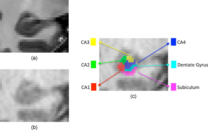
In this paper, we propose to use 3T multi-modality MR images (3T T1 MRI, 3T T2 MRI, and 3T rs-fMRI) to automatically segment hippocampal subfields (including the subiculum (Sub), CA1, CA2, CA3, CA4, and dentate gyrus (DG), see Fig. 1). Besides exploring appearance patterns from structural MRI (T1 and T2 MRI), we also explore connectivity patterns of different subfields from rs-fMRI for helping segmentation. The appearance features and relationship features are extracted to capture the appearance patterns in structural MRI as well as the connectivity patterns in rs-fMRI, respectively. These extracted features are inputted to the structured random forest (Kontschieder et al., 2011) and auto-context (Loog and Ginneken, 2006; Tu and Bai, 2010) off-line learning framework (Qian et al., 2016) for training. Then, a segmentation classifier can be constructed. When a testing image comes, its corresponding appearance features and relationship features are extracted and then fed into the learned classifier for segmentation. The segmentation performance is quantitatively compared to the manual labels using Dice ratio. To the best of our knowledge, this is the first paper that explores the functional connectivity patterns to assist hippocampal subfields segmentation. The proposed method is tested on two datasets, and the experiments show that the features from multi-modality images improve the hippocampal subfields segmentation performance. On the other hand, our method may be limited for certain applications since it requires the rs-fMRI, which is currently not as universally available as the structural MRI, such as T1 or T2 MRI. However, as the fMRI and connectivity patterns become more and more popular (Glasser et al., 2016b,a), the rs-fMRI would be acquired for more clinical cases in the future.

Figure 1.

Illustration of hippocampal subfields. (a) The 7T T1 MRI of the right hippocampus, with distinct subfield boundaries. (b) 3T T1 MRI of the same hippocampus from the same subject, with ambiguous subfield boundaries. (c) Six manually labeled hippocampal subfields overlapped on 3T T1 MRI.

This paper significantly extends our previous workshop paper (Wu et al., 2016) in the following aspects. a) More details of the method are provided; b) Experiments on newly labeled dataset (4 subjects) from the HCP dataset (Van Essen et al., 2013) are also included to evaluate the benefits of employing multi-modality features from 3T T1, 3T T2, and 3T rs-fMRI data. Previously, we only used 3T T1 MRI and 3T rs-fMRI; c) More comparisons with state-of-art methods are also included.

The rest of the paper is organized as follows. Section 2 provides the whole framework and method details, including feature extraction in multi-modalities, classifier building, and auto-context learning framework for iterative segmentation refinement. In Section 3, experimental results and related quantitative analysis are reported. Finally, Section 4 concludes the paper.

2. Main framework

2.1. Motivation

The main challenge of subfield segmentation on 3T MRI is the ambiguous subfield boundary caused by limited image quality. Fig. 1 (b) demonstrates a typical routine 3T T1 MRI of hippocampal subfields. Due to such ambiguity, the appearance patterns from two different subfields might be similar, which could lead to inaccurate segmentation. In order to compensate such ambiguity, we introduce the 3T rs-fMRI to capture the connectivity patterns among the subfields and use the difference of these patterns to facilitate the segmentation of patches even with similar appearance.

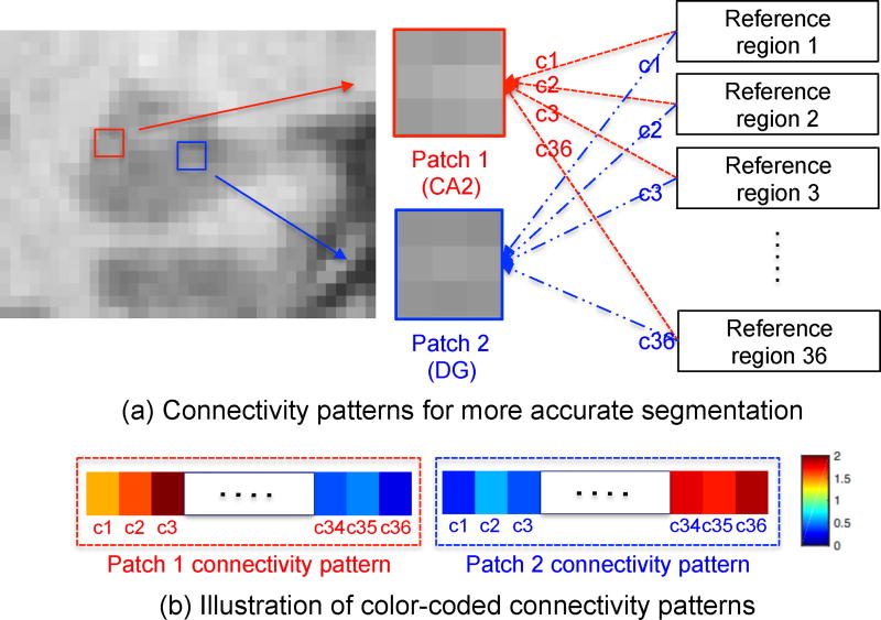
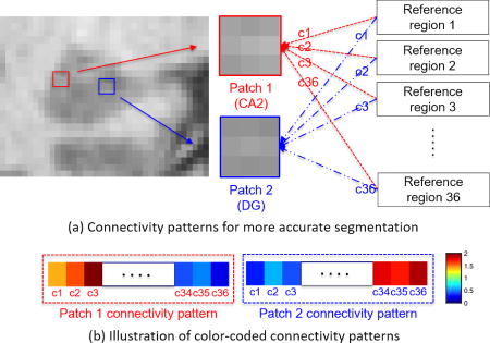
Fig. 2 (a) illustrates our main idea. Patch 1 (belonging to CA2) and patch 2 (belonging to DG) are quite similar in 3T T1 MRI. It’s difficult to determine their subfield labels if using only appearance patterns. However, their connectivity patterns (i.e., functional connectivity) between each patch and reference regions {c₁, c₂, …, c₃₆} (where 36 is the total number of reference regions used in our study) in the rs-fMRI are different, as illustrated in Fig. 2 (b). Thus, we can potentially distinguish these two patches through the differences of their connectivity patterns.

Figure 2.

The illustration of using connectivity patterns in rs-fMRI for segmentation. (a) To distinguish the two appearance-similar patches in T1 MRI, we utilize the relationship features extracted from connectivity patterns in rs-fMRI. (b) The color-coded connectivity patterns of patch 1 and patch 2 are illustrated.

The details of the method are covered in the following 4 subsections. Subsection 2.2 explains the data preprocessing, including manual label generation and also alignment from other modality images to 3T T1 MRI. Subsection 2.3 elaborates how appearance features and relationship features are extracted to capture the appearance patterns and connectivity patterns, respectively. In subsection 2.4, structured random forest classifier is introduced, which is used as our segmentation classifier. Subsection 2.5 introduces our unified structured random forest and auto-context segmentation framework, in which the trained classifier and the segmentation results are consistently refined.

2.2. Data preprocessing

2.2.1. Manual label generation

To get the training data, for each subject in our two datasets, 6 hippocampal subfields are manually labeled. In the first dataset, due to the low image resolution and low signal contrast of 3T T1 MRI, the boundaries of hippocampal subfields are not clear. In order to get better training data, we use 7T T1 MRI to help generate the manual labels for the 3T T1 MRI. First, for each subject, we up-sampled the 3T T1 MRI to the resolution of 0.65mm isotropic, which is the same as the resolution of 7T T1 MRI. Then, we linearly align the 7T T1 MRI onto the up-sampled 3T T1 MRI using Flirt (Jenkinson et al., 2002), which is a linear image registration toolkit that is efficient for the task of cross-modality image registration of the same subject. By doing so, we get the aligned 7T T1 MRI with similar resolution and signal contrast as the original 7T T1 MRI, but sitting in the 3T T1 MRI space. Then, six subfields are manually delineated on the aligned 7T T1 MRI. For the images in the second dataset, the manual labeling is directly conducted on each 3T T1 MRI, and cross-checked using 3T T2 MRI. The reasons for doing so is because a) their resolution and quality are relatively good; b) the T1 and T2 MRI have already been aligned well by the well-validated preprocessing pipeline in (Van Essen et al., 2013). In the supplementary materials, we explain the detailed steps for conducting manual labels, and present further statistical information about manual labels.

2.2.2. Register rs-fMRI to T1 MRI

For subjects in the first dataset, since their 3T T1 MRI and 3T rs-fMRI are in different spaces, we need to align them into the same space (3T T1 MRI space) for extracting corresponding features. For the T1 MRI data, non-brain tissues such as skull and dura are first stripped (Shi et al., 2012) and then intensity inhomogeneity is corrected through N3 correction (Sled et al., 1998). For rs-fMRI data, the SPM toolkit (Penny et al., 2011) is used for preprocessing, including discarding the first 10 volumes, slice timing correction, rigid-body motion correction, band pass filtering, and signal regression of white matter, CSF, and six motion parameters. Finally, we register the preprocessed rs-fMRI data onto their corresponding T1 image for each subject.

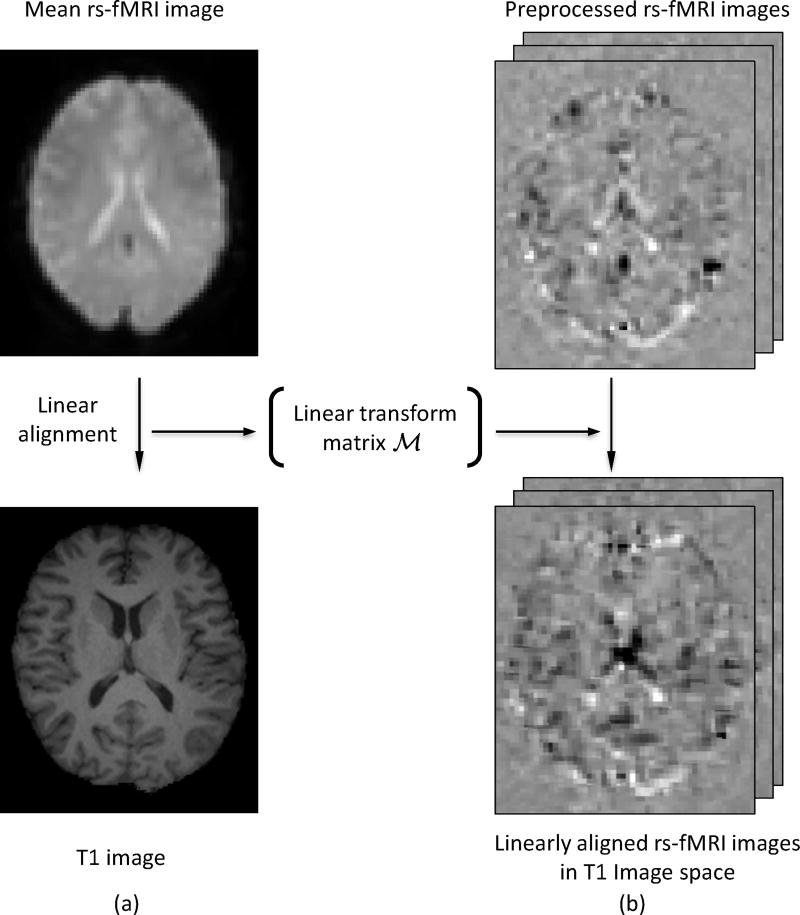
Unlike the conventional way of co-registering each single volume of rs-fMRI data separately to the T1 MR image, which may generate temporary inconsistency between neighboring fMRI frames, we employ a two-step approach to improve the temporary consistency of registration, as illustrated in Fig. 3. First, the mean rs-fMRI image is computed and linearly registered to the corresponding T1 MR image to get the linear transform matrix ℳ, see Fig. 3 (a). Second, the obtained transform matrix ℳ is applied to the preprocessed rs-fMRI images and brings them to the T1 MRI space using the nearest neighbor interpolation. After that, the rs-fMRI and T1 MRI are sitting in the same space, and features extracted from both modalities are now in correspondence and can be used together.

Figure 3.

Registration of the rs-fMRI to the T1 MRI for building their correspondences.

In the second dataset, the HCP preprocessing pipeline (Van Essen et al., 2013) has already aligned all the 3T T1, 3T T2, and 3T rs-fMRI into the common space. So we can directly use the aligned data for feature extraction.

2.3. Feature extraction

2.3.1. Appearance features from 3T T1 and T2 MRI

The appearance features are extracted from 3T T1 and 3T T2 MRI to capture appearance patterns for different subfields. The histogram matching (Nyúl et al., 2000) is adopted to match the histogram of all subjects to the histogram of the template for T1 and T2 MRI, respectively. Note that the template is selected by the following steps. First, we calculate the histogram for each image (either T1 or T2 MRI), and obtain the mean histogram from all images. Then, we select the one with the minimal distance of its histogram to histograms of all other images as the template. From each histogram-matched image, two kinds of appearance features are extracted, i.e., the gradient-based texture features and 3D Haar features.

The gradient-based texture features include features from the first-order difference filters (FOD), the second-order difference filters (SOD), 3D hyperplane filters, 3D Sobel filters, Laplacian filters, and range difference filters. The total number of texture features is 36 (Hao et al., 2014). The 3D Haar feature is an extension of 2D Haar feature, with the calculation unit expanded from boxes to cubes, which can also be calculated efficiently through the 3D integral image. More details can be found in (Ke et al., 2005).

On 3T T1 and 3T T2 MRI, for each image patch (11×11×11 in our experiments), the above texture feature set (36 features) and 3D Haar feature set (2000 features) are extracted, which are used as appearance features.

2.3.2. Features from rs-fMRI

The relationship features are extracted to capture connectivity patterns for different subfields. For any local patch (with patch size of 11×11×11), its connectivity patterns can be regarded as the Pearson correlation of the mean BOLD signals between this patch and some reference regions. Thus, even for the appearance-similar patches, if their relationship features from the connectivity patterns are different, they can still be distinguished.

Based on the above idea, we need to address the following two problems: a) how to select reference regions to formulate connectivity patterns, and b) how to extract relationship features to capture the information in the connectivity patterns. We address the above two problems in the following 4 steps: a) reference regions construction; b) connectivity patterns construction; c) connectivity patterns discrimination with subfield prior; and d) relationship features extraction from discriminative connectivity patterns.

Reference region construction

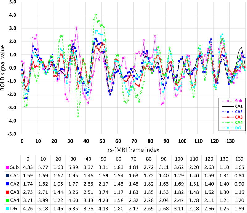
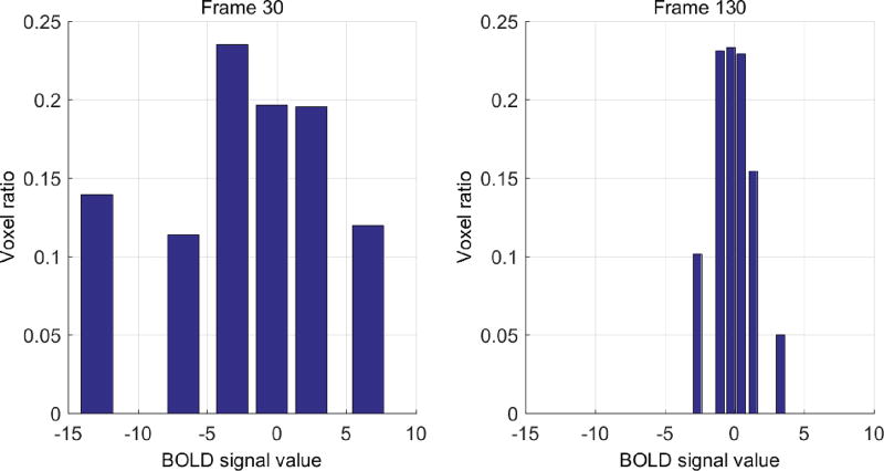
For different subfields, a rational assumption is that the BOLD signals are highly correlated inside the same subfield, but less correlated across different subfields. The traditional way is to use each subfield as a reference region to build the connectivity patterns. However, this may be too coarse and thus lots of valuable information would be ignored. Fig. 4 demonstrates the mean (in figure) and standard deviation (in table) of rs-fMRI BOLD signals of different subfields for one subject. The horizontal axis of the figure is the index of rs-fMRI frame, and the vertical axis denotes the magnitude of the BOLD signals. The table under the figure shows the standard deviation, with the first row indicating the index for the frame. From the figure, we can see that the mean BOLD signals of these subfields share similar overall patterns. However, in the table, we can see that the standard deviation of BOLD signals within a subfield is not necessarily small (even compared to the maximum magnitude of mean BOLD signals). This high standard deviation indicates more information to explore. This also means that using a single mean signal to represent the signals of the whole subfield would over-smooth useful information, especially when the distribution of BOLD signals is not at a single Gaussian fashion. The fact is that the distribution of BOLD signals in the entire subfield cannot be regarded as single Gaussian in many fMRI frames. As shown in Fig. 5, in fMRI frame 30, the BOLD signals of subfield Sub (subiculum) are more likely distributed uniformly.

Figure 4.

Mean BOLD signals of 6 different subfields (upper panel) and their corresponding standard deviations in selected frames (bottom table).

Figure 5.

BOLD signal distributions of subfield Sub (Subiculum) in 2 frames (left and right panels in figure).

To explore more information, for each subfield, we further divide it into several subregions and use the signal set of all subregions, rather than a single mean signal, to build the connectivity patterns. Specifically, the division is implemented by clustering. The clustering objective here is to group voxels with similar BOLD signals and closer spatial distance into the same cluster. In our current implementation, we use a straightforward random search strategy to get a local optimal solution. First, the 3D position vector of each voxel is fed into the k-means clustering procedure (Hartigan and Wong, 1979), with randomly initialized cluster centers (where each cluster center corresponds to a subfield division). Then, for each division, the sum of standard deviations of the BOLD signals can be calculated, and the one with the minimal sum is selected accordingly.

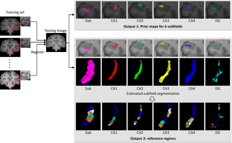
However, for a testing subject, each subfield location has not been determined yet. Thus, the question of how to further divide it into subregions remains unsolved. To address this problem, we first estimate each subfield and then divide it into subregions. Specifically, for a testing subject, the multi-atlas and majority voting strategy (Wang et al., 2013) is used to roughly estimate an initial subfield segmentation. This procedure is briefed as follows. First, all training images $\{I_1^{\mathit{\text{tr}}},\cdots ,I_M^{\mathit{\text{tr}}}\}$ are nonlinearly registered onto a testing image I^te for obtaining the respective deformation fields {D₁, ⋯, D_M}, where M is the number of training images. Then, these deformation fields are applied to the respective label images $\{L_1^{\mathit{\text{tr}}},\cdots ,L_M^{\mathit{\text{tr}}}\}$ to obtain the subfield prior (SP) maps, which is simply the probability map for each subfield label, e.g., Output 1 of prior maps for 6 subfields in Fig. 6. Moreover, through the majority voting, an initial subfield segmentation can be obtained too, e.g., the estimated subfield segmentation in Fig. 6. Note that, for a training image, although each subfield has already been labeled, we still use the above strategy to estimate an initial subfield rather than using the labeled one, i.e., using the other M-1 training images to estimate the initial subfield segmentation. This means, the labels of the training images are just used for classifier training, not involved in the reference regions partition, for making it consistent with testing image.

Figure 6.

The schematic illustration of reference regions construction.

Once the initial subfield for training and testing images are estimated, using the aforementioned clustering strategy, we further divide each subfield into 6 subregions, as shown in Output 2 of reference regions in Fig. 6. To make the division of each subfield consistent across different subjects, the division is first carried on one randomly selected training image as template to obtain the centroids of the divided subregions. Then, these centroids are non-linearly registered to all other images. Thus, the subfield in the new image can be divided by assigning each voxel to the subregion with the nearest distance.

Using the k-means to partition the whole subfield into subregions is a typical Voronoi tessellation problem. In certain case, with very bad initialization for the k-means, one subregion might only contain 1 voxel. However, because the clustering is only conducted on the template image space, we could directly exclude the partition that certain subregion has too few voxels (i.e., less than 2% of the voxel number of whole subfield in the experiment). Compared to other strategies such as spectral clustering, this strategy is quite simple and efficient. Therefore, we could run many rounds of searching to get a majority-voted solution for robustness.

The advantages of the subdivision include: a) Each subregion has smaller standard deviation of BOLD signals than that of the entire subfield, thus reducing the negative impact of over-smoothing if using the entire subfield; b) The roughly estimated subfields that generated by the multi-atlas and majority voting strategy might contain some mislabeled voxels. But, after partitioning the estimated subfield into subregions, in some subregions, the mislabeled voxels number could be decreased. Then, the BOLD signals from these subregions could be better used as the reference for building the connectivity patterns, since they suffer less from the noisy signals.

Connectivity pattern construction

Once the reference regions are determined, the reference BOLD signals can be obtained by averaging BOLD signals over each reference region. Then, the connectivity pattern for each voxel can be calculated as follows.

For each subject, we first calculate 36 (6 subregions from each of 6 subfields) sets of reference BOLD signals, denoted as ${\mathbf{b}}_k^R$, k = 1, …, 36. Then, for any voxel r, we extract its local patch in rs-fMRI and calculate the mean BOLD signal, denoted as b(r). The connectivity pattern between this local patch and the reference regions is denoted as c_k (r), k = 1, …, 36, which is calculated by the Pearson correlation coefficients between b(r) and ${\mathbf{b}}_k^R$.

$$c_k(r)=\frac{\mathit{\text{cov}}(\mathbf{b}(r),{\mathbf{b}}_k^R)}{{\sigma }_{\mathbf{b}(r)}{\sigma }_{{\mathbf{b}}_k^R}}+1$$

where cov(b(r), ${\mathbf{b}}_k^R$) is the covariance, and σ_b(r) and ${\sigma }_{{\mathbf{b}}_k^R}$ are the standard deviations of b(r) and ${\mathbf{b}}_k^R$. Here, the reason to add 1 is to make the connectivity pattern non-negative, and note that this shift will not influence the final classification because all c_k(r) are equivalently shifted.

Through the above operations, for any voxel r, we get a connectivity pattern vector {c_k(r), k = 1, …, 36}, which captures the relationship between this voxel and each reference region, where {c_k(r), k = 1, …, 6} captures relationships from local patch to Sub., and {c_k(r), k = 7, …, 12} captures relationships from local patch to CA1, etc.

Connectivity pattern discrimination with prior

We can further increase the discrimination of the above connectivity pattern using the subfield prior. Supposing that there are two voxels, i.e., voxel s and t with s belonging to CA1 and t belonging to CA2. Their corresponding connectivity patterns can be denoted as:

$$\mathbf{c}(s)=\{c_k(s),k=1,\dots ,36\}$$

$$\mathbf{c}(t)=\{c_k(t),k=1,\dots ,36\}$$

Considering the fact that each subfield is relatively small, the difference between these two voxels’ connectivity patterns 𝒟(c(s), c(t)) might be subtle, which is less beneficial for classification. Therefore, we employ the subfield prior to enhance their difference as detailed below.

For any voxel r, let p^Sub(r), p^CA1(r), p^CA2(r), p^CA3(r), p^CA4(r), p^DG(r) denote its probabilities belonging to 6 different subfields, which are the output of atlas registration, as described in Section 2.3.2. Note that these probabilities will be updated in the segmentation process, which will be described in Section 2.5. These probabilities can be used to weight the corresponding connectivity pattern. And the weighted connectivity pattern v(r) = {υ _k(r)|k = 1, …, 36} of voxel r is:

$$\{{\upsilon }_k(r)\}=\left\{\begin{array}{cc}{p}^{\text{Sub}}(r)\ast c_k(r),\hfill & k=1,\dots ,6\hfill \\ p^{\text{CA}1}(r)\ast c_k(r),\hfill & k=7,\dots ,12\hfill \\ p^{\text{CA}2}(r)\ast c_k(r),\hfill & k=13,\dots ,18\hfill \\ p^{\text{CA}3}(r)\ast c_k(r),\hfill & k=19,\dots ,24\hfill \\ p^{\text{CA}4}(r)\ast c_k(r),\hfill & k=25,\dots ,30\hfill \\ p^{\text{DG}}(r)\ast c_k(r),\hfill & k=31,\dots ,36\hfill \end{array}\right\}$$

The above formula is quite straightforward. If the subfield prior indicates that the center voxel r of this patch more likely belongs to CA1 than other subfields, its connectivity to CA1 are enhanced, while the connectivity to other subfields are suppressed. This weighting strategy could suppress the noises when we calculate the connectivity patterns and also make these patterns more discriminative for classification.

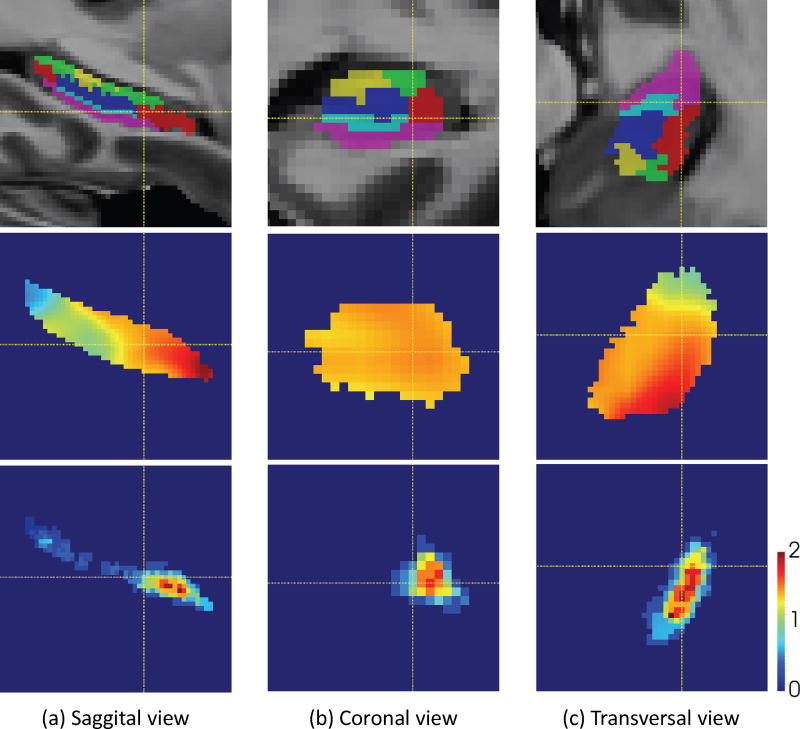
Fig. 7 shows the enhanced connectivity pattern corresponding to the first subregion of subfield CA1. The first row shows the manual label of each subfield, with the red color indicating CA1. The second row shows the connectivity pattern before incorporating the subfield prior. And, the last row shows the enhanced connectivity pattern by incorporation of subfield prior. From the figure, it can be seen that the enhancement could strengthen the signal contrast along the subfields boundary. With better contrast, the segmentation performance could be better.

Figure 7.

The enhancement of the connectivity pattern by subfield prior. The first row shows the manual label of each subfield, and the red color indicates the CA1; The second row shows the connectivity pattern corresponding to the first subregion of subfield CA1 before adding the subfield prior; While the last row shows the connectivity pattern after enhanced by the subfield prior. The yellow cross indicates the same position at different views.

Relationship features extraction from connectivity pattern

Using the above strategy, for any testing image, we can obtain 36 connectivity pattern maps. Each voxel of the k-th connectivity pattern map corresponds to the weighted connectivity from this voxel to the k-th reference region. In order to capture the connectivity patterns for classification, the 3D Haar features are further extracted from the 36 connectivity pattern maps. In our experiments, for each voxel, a local patch with size 11×11×11 is extracted, and then 100 Haar features are extracted from each connectivity pattern map. Thus, totally 36×100 = 3600 Haar features are extracted for each voxel, and they are used as the relationship features.

2.4. Structured random forest classifier

After extracting the appearance features from structural MRI and relationship features from rs-fMRI, we concatenate them to formulate a feature set for learning a structured random forest (Kontschieder et al., 2011; Criminisi et al., 2012; Criminisi and Shotton, 2013) classifier.

The input of the structured random forest for a local voxel i, is the feature vector x_i and its label vector l_i. The label vector is denoted as l_i = {y_i}∪{y_j|j ∈ 𝒩_i}, where y_i is the label of i, {y_j|j ∈ 𝒩_i} is its neighbors’ labels, and 𝒩_i is the neighbors of i. y_i, y_j ∈ ℒ, and ℒ = {1, 2, …, 6} is the label set corresponding to 6 subfields considered in this work. Because labels of both center voxel and its neighboring voxels are used together as supervised information, the structured random forest can potentially capture the local structure of the predicted voxel. With the training vector pair (x_i, l_i), the best split at each node is selected as the one with maximal information gain for the center voxel and neighboring voxels. After training, the prediction of testing voxel i is also a label vector {(ŷ_i)} ∪ {(ŷ_j)|j ∈ N_i}, where ŷ_i is the predicted label of the testing voxel i and {y_j|j ∈ 𝒩_i} are the predicted label of its neighboring voxels. By voxel-wise label prediction, each testing voxel could have multiple estimated labels, which will be then fused by majority voting.

2.5. Structured random forest and auto-context segmentation framework

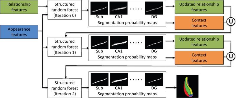
The structured random forest (Kontschieder et al., 2011) and auto-context model (Loog and Ginneken, 2006; Tu and Bai, 2010) are combined together to further refine the segmentation in an iterative manner during the training and testing stages. The entire process is illustrated in Fig. 8 and detailed below.

Figure 8.

The segmentation refinement via the auto-context model. Note that the 36 connectivity pattern maps will be updated iteratively as well, which are used to update the relationship features.

During the training stage, in iteration 0, the appearance features and relationship features extracted from the training images are used to train a structured random forest. Then, the trained classifier is applied to each training image, and 6 segmentation probability maps corresponding to 6 subfields (see Fig. 8) are obtained. These segmentation probability maps are used to extract the context features and also update the relationship features. The context features are extracted as the 3D Haar features directly from the segmentation probability maps, which are the high-level features characterizing the neighboring label prediction. The relationship features are computed as follows. First, the 6 segmentation probability maps are binarized into the 6 subfield segmentations with a threshold (0.5). Then, each segmented subfield is further divided to produce the updated reference regions, which will update the connectivity pattern maps and thus the relationship features. In the next iteration (iteration 1), the context features together with the updated relationship features and the original appearance features are used to train a new structured random forest. This procedure is repeated iteratively and, in each iteration, the classifier is refined.

During the testing stage, in iteration 0, the appearance features and relationship features extracted from the testing image are fed into the trained classifier of this iteration, to predict 6 segmentation probability maps. Then, according to the predicted segmentation probability maps, we can update the reference regions and then the relationship features. And also the context features are extracted from these predicted probability maps. In iteration 1, the original appearance features, context features, and updated relationship features are fed into the classifier of iteration 1, to obtain the refined segmentation probability maps. Then, the relationship features can thus be updated. This procedure is repeated iteratively. In the last iteration, to finalize the segmentation, we first treat all 6 subfields as a single foreground by summing up all 6 probability maps to produce a foreground probability map. Then, we threshold it (with 0.5) to obtain the foreground segmentation map, which can be used as a mask for the 6 probability maps. That is, only voxels inside the foreground segmentation map are considered, and their labels are finally determined by a respective subfield label with maximum probability.

3. Experiments

3.1. Materials and experiment configuration

Two datasets are used in the experiments. For each subject in two datasets, six hippocampal subfields (including the Sub, CA1, CA2, CA3, CA4, and DG) of both left and right hippocampus are manually delineated by an expert neuroradiologist. The first dataset includes 8 healthy subjects (with ages of 30 ± 8 years). Each subject has 7T T1 MRI, 3T T1 MRI, and 3T rs-fMRI. A Siemens Trio 3T scanner collected the 3T T1 MRI and 3T rs-fMRI. The Siemens Magnetom 7T scanner collected the 7T T1 MRI. The 3T T1 MRI is collected by an MPRAGE sequence with parameters: TR=1900ms, TE=2.16ms, TI=900ms and isotropic 1mm resolution. The 3T rs-fMRI uses a gradient-echo EPI sequence with parameters: TR=2000ms, TE=32ms, FA=80, matrix=64×64, resolution=3.75×3.75×4mm³. A total of 150 volumes are obtained by 5mins. The 7T T1 MRI is collected by an MPRAGE sequence with parameters of TR=6000ms, TE=2.95ms, TI=800/2700ms and with isotropic 0.65mm resolution. The second dataset includes 4 healthy subjects, selected randomly from the preprocessed HCP 500 released dataset, where 3T T1, T2, and rs-fMRI have already been preprocessed (Van Essen et al., 2013). For 3T T1 and T2 MRI, the resolution is isotropic 0.7mm; for the rs-fMRI, the resolution is isotropic 2mm.

The Dice ratio between the automatic segmentation and the manual label is used as quantitative measurement of the segmentation performance, and the leave-one-out strategy is adopted in each dataset to evaluate the performance.

3.2. Segmentation performance analysis

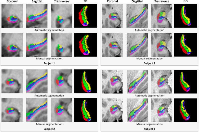
The results of left hippocampal subfields segmentation of 4 subjects are demonstrated in Fig. 9 by overlapping the automatic segmentation and manual labels on their 3T T1 MRI, respectively. Among them, subjects 1 and 2 are from the first dataset, while subjects 3 and 4 are from the second dataset. Although the resolutions and signal contrasts of both structural MRI and rs-fMRI are different in these two datasets, it can be seen that the proposed method can effectively segment hippocampal subfields in both datasets consistently with the manual labels.

Figure 9.

Subfield segmentation results for four subjects from two datasets (left hippocampus).

From Fig. 9, it can be seen that our segmentation appears less bumpy than the manual labeling. For the manual labeling, the radiologist first delineates each subfield slice by slice on the image, and then refines the delineation in three different views (i.e., sagittal, coronal and transversal views), respectively. However, the smooth boundary labeled in one view usually appears to be non-smooth in other two views. Even based on the 2D slice-by-slice refinement, some bumpy boundaries in 3D space are still inevitable. On the other hand, the automatic method can extract both appearance and relationship features directly from the 3D patches by considering spatial information in 3D space. In addition, the structured random forest predicts the labels for the local patch, which also preserves the local structure of labeling results. Therefore, automatic segmentation looks more consistent, which can also be considered as one of the advantages of our method.

The quantitative analysis of the first dataset is given in Table 1 and Table 2. Each entry in Table 1 shows the mean ± standard deviation of the Dice ratios in the leave-one-out cross-validation, and each entry in Table 2 provides the true positive rate (TPR) and the true negative rate (TNR). In this experiment, we extracted 2036 features from 3T T1 MRI and 3600 relationship features from 3T rs-fMRI. From the table, we can see, by combining the 3T T1 MRI and 3T rs-fMRI, the segmentation results are significantly improved (with p=0.0004, β=0.01 when α=0.05) and consistently better than those only using 3T T1 MRI, with both the increased mean Dice ratio and decreased standard deviation. The consistent increase in the mean Dice ratio indicates that the relationship features from 3T rs-fMRI provide complementary information, which effectively benefits for the subfield segmentation. In addition, the consistent decrease of standard deviation also means that, using multi-modality data, the segmentation results are more robust. Besides, we also compared with the results obtained by the multi-atlas registration plus majority voting (MA+MV) (Wang et al., 2013) on 3T and 7T T1 MRI, respectively. All these comparison results indicate that the appearance features and relationship features can successfully capture the appearance and connective patterns of different hippocampal subfields for segmentation, using the proposed structured random forest and auto-context learning framework.

Table 1.

Segmentation performance on the first dataset. Bolded numbers indicate the best performance using 3T image modalities.

Dice (Mean±Std.)	Sub.	CA1	CA2	CA3	CA4	DG
MA+MV on 3T T1	0.52±0.17	0.49±0.15	0.48±0.09	0.49±0.10	0.53±0.10	0.44±0.23
Only 3T T1	0.63±0.15	0.64±0.17	0.63±0.14	0.65±0.11	0.66±0.15	0.53±0.13
rs-fMRI	0.61±0.13	0.65±0.11	0.62±0.07	0.61±0.08	0.64±0.08	0.46±0.15
3T T1+3T rs-fMRI	0.68±0.05	0.68±0.10	0.66±0.06	0.67±0.06	0.69±0.05	0.57±0.10
MA+MV on 7T T1	0.65±0.07	0.62±0.13	0.60±0.12	0.56±0.14	0.63±0.08	0.52±0.12
Only 7T T1	0.75±0.04	0.68±0.09	0.68±0.04	0.68±0.06	0.72±0.04	0.65±0.09
7T T1+3T rs-fMRI	0.75±0.04	0.69±0.07	0.68±0.05	0.68±0.05	0.72±0.04	0.63±0.11

Table 2.

Segmentation performance evaluation in TPR/TNR on the first dataset.

TPR/TNR	Sub.	CA1	CA2	CA3	CA4	DG
MA+MV on 3T T1	0.60/0.92	0.53/0.93	0.52/0.94	0.54/0.95	0.60/0.93	0.51/0.94
Only 3T-T1	0.69/0.92	0.65/0.94	0.69/0.95	0.66/0.96	0.71/0.93	0.58/0.95
rs-fMRI	0.67/0.90	0.70/0.93	0.72/0.94	0.69/0.95	0.68/0.92	0.53/0.93
3T T1+3T rs-fMRI	0.74/0.91	0.71/0.93	0.71/0.94	0.69/0.95	0.71/0.93	0.63/0.95
MA+MV on 7T T1	0.72/0.93	0.68/0.94	0.65/0.94	0.61/0.95	0.67/0.93	0.60/0.94
Only 7T T1	0.75/0.93	0.71/0.93	0.72/0.94	0.69/0.95	0.72/0.93	0.63/0.95
7T T1+3T rs-fMRI	0.76/0.92	0.74/0.94	0.72/0.95	0.68/0.95	0.73/0.93	0.64/0.95

Quantitative results of the second dataset are presented in Table 3 (Dice ratio) and Table 4 (TPR and TNR). Each structural modality (T1, T2) and their combinations with rs-fMRI are used to validate our method. From the table, it can be seen, a) in the case of using two modalities, by introducing the rs-fMRI, the performance of segmenting subfields using T1+fMRI or T2+fMRI is significantly improved in terms of Dice ratio, compared to the case of using only the single structural modality image (with p=0.0063, β=0.06 when α=0.05 for T1+fMRI vs. T1, and p=0.0099, β=0.11 when α=0.05 for T2+fMRI vs. T2). Besides, the segmentation performance of T1+T2 is significantly improved compared to the case of using either T1 (with p=0.0003, β=0.02 when α=0.05 for T1+T2 vs. T1) or T2 (with p=0.0002, β=0.06 when α=0.05 for T1+T2 vs. T2). b) In the case of using three modalities, the segmentation performance of T1+T2+fMRI is better than using any of the two modality combinations. For example, the segmentation performance of T1+T2+fMRI is significantly better than the segmentation of T1+fMRI (with p=0.0004, β=0.01 when α=0.05) and T2+fMRI (with p=0.0014, β=0.02 when α=0.05). Compared to the result of T1+T2, the segmentation performance of T1+T2+fMRI is also significantly improved (with p=0.015, β=0.18 when α=0.05); For example, for CA3 and CA2, the increase is 0.03 in Dice ratio.

Table 3.

Segmentation performance on the second dataset. Bolded numbers indicate the best performance using 3T image modalities.

Dice (Mean±Std.)	Sub.	CA1	CA2	CA3	CA4	DG
MA+MV on T1	0.59±0.12	0.60±0.18	0.53±0.13	0.46±0.12	0.51±0.16	0.46±0.16
Only T1	0.65±0.03	0.68±0.04	0.61±0.05	0.51±0.04	0.60±0.06	0.53±0.05
Only T2	0.66±0.04	0.70±0.03	0.61±0.04	0.51±0.06	0.61±0.04	0.52±0.04
T1+T2	0.69±0.04	0.73±0.03	0.63±0.05	0.54±0.04	0.63±0.05	0.56±0.04
T1+fMRI	0.67±0.05	0.72±0.03	0.63±0.06	0.55±0.04	0.62±0.06	0.53±0.05
T2+fMRI	0.68±0.04	0.71±0.03	0.62±0.04	0.55±0.05	0.62±0.04	0.53±0.05
T1+T2+fMRI	0.69±0.05	0.74±0.02	0.66±0.03	0.57±0.03	0.64±0.04	0.57±0.05

Table 4.

Segmentation performance evaluation in TPR/TNR on the second dataset

TPR/TNR	Sub.	CA1	CA2	CA3	CA4	DG
MA+MV on T1	0.64/0.92	0.64/0.94	0.57/0.95	0.50/0.95	0.59/0.93	0.55/0.94
Only T1	0.69/0.93	0.74/0.96	0.67/0.96	0.52/0.96	0.68/0.92	0.60/0.95
Only T2	0.73/0.93	0.74/0.96	0.66/0.96	0.57/0.96	0.69/0.92	0.61/0.95
T1+T2	0.77/0.93	0.80/0.95	0.69/0.96	0.60/0.96	0.71/0.92	0.62/0.95
T1+fMRI	0.76/0.92	0.79/0.94	0.69/0.95	0.56/0.95	0.70/0.93	0.61/0.95
T2+fMRI	0.76/0.92	0.78/0.94	0.69/0.95	0.58/0.95	0.69/0.93	0.60/0.95
T1+T2+fMRI	0.78/0.92	0.82/0.94	0.74/0.95	0.64/0.96	0.73/0.93	0.64/0.95

It is worth noting that the TNR is stable for different methods, due to the small size of the hippocampal subfields compared to the size of background voxels in the classification. From the quantitative experimental results of the two datasets, it can be seen that the complementary information from multimodality images effectively improves the hippocampal subfields segmentation in the same dataset. However, the two datasets have different subject number and different image quality, i.e., the first dataset has two times subject number than the second dataset, while the second dataset has better image quality. This might cause performance difference between two datasets; For example, the segmentations of two subfields using T1+T2+fMRI from the second dataset are worse than the respective segmentations using T1+fMRI from the first dataset. Considering the dataset differences, we couldn’t draw conclusion from cross-dataset comparison. In the experiments, the patch size 11×11×11 is used for both datasets to extract the appearance and relationship features, and it is selected by cross-validation. The reason that this patch size (11×11×11) works better for both datasets might due to the similar resolutions of the two datasets (i.e., 0.65mm and 0.7mm isotropic, respectively).

3.3. Multi-modality vs. ultra-high magnetic field strength

We have also compared the subfield segmentation using 3T multi-modality MR images with that using 7T T1 MRI in two experiments. In the first experiment, we segment subfields in the 7T T1 MRI by using the same appearance features as the 3T T1 MRI, i.e., the gradient-based texture features and 3D Haar features. In the second experiment, we combine the appearance features from 7T T1 MRI and relationship features from 3T rs-fMRI for subfield segmentation. Both results are reported in last two rows of Table 1. It can be seen that the combination of 7T T1 MRI with 3T rs-fMRI yields the segmentation performance that is almost the same with the case of using only the 7T T1 MRI. This implies that the relationship features from 3T rs-fMRI do not provide benefits for subfield segmentation, because the ground-truth was defined on the 7T data. Comparing row 6 with row 7, it can be seen that by using the complementary features from 3T T1 and 3T rs-fMRI, the segmentation results (CA1 – CA4) are comparable to those obtained by using only the 7T T1 MRI. However, for the subiculum (Sub) and dentate gyrus (DG), more detailed appearance patterns from 7T T1 MRI seems very beneficial, thus the results on 3T multi-modality images are inferior.

3.4. ACM performance evaluation

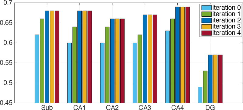
We adopted the auto-context model to iteratively refine the segmentation results. The result of each iteration on the first dataset is reported in Fig. 10 (with the mean of Dice ratios). From the figure, it can be seen that the auto-context model is quite effective in refining the segmentation results, especially in the first two iterations. There are two reasons: a) in each iteration, the previous segmentation result provides tentative label predictions of neighboring voxels, which can be used to learn the structure information of neighboring predictions. This information helps refine voxel-wise segmentations that are performed independently; b) the refined segmentation leads to refined reference regions, which updates the relationship features that are capable of capturing the connectivity patterns of different subfields. Thus, the segmentation is further refined. In our case, the segmentation results become stable after the 2nd iteration, so we used 2 iterations for all results reported in this paper.

Figure 10.

Subfield segmentation results (mean Dice ratio) at different auto-context iterations.

3.5. Discussion

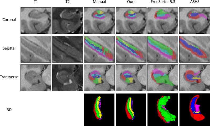
We also apply the state-of-the-art methods on our second dataset, including the FreeSurfer (Van Leemput et al., 2009) and ASHS (Yushkevich et al., 2015b). The segmentation results are provided in Fig. 11. From the figure, it can be seen that, although three methods successfully segment the hippocampal subfields, the segmentation results have some differences. The main reason is the use of different hippocampus subfields partition protocols by different methods.

Figure 11.

Comparison of state-of-the-art methods in segmenting one subject from the second dataset.

The precise neuroanatomy of hippocampal subfields definition relies on the cytoarchitecture of the hippocampus. However, the resolution of the MR images could not reach the cytoarchitecture level. Therefore, the radiologists’ prior knowledge becomes essential in labeling subfields on MR images, which thus leads to inconsistent labeling protocols for hippocampal subfields in the field (Boccardi et al., 2011; Yushkevich et al., 2015a). These protocols differ from each other in two aspects. a) There is no consensus on how many subfields should be partitioned in the hippocampus. In most cases, the number of subfields is dependent on different applications. b) The boundary locations of different subfields are subjective and highly dependent on the expertise, since different neurologists may rate different boundaries. These two issues have been explicitly discussed in many works (Boccardi et al., 2011, 2015; Yushkevich et al., 2015a; Wisse et al., 2017). For example, in the FreeSurfer segmentation, the whole hippocampus is partitioned into 4 subfields. CA2 and CA3 are treated as a single subfield CA2/3. CA4 and DG are also treated as a single CA4/DG. While, in the ASHS segmentation, the whole hippocampus is partitioned into 5 subfields, by treating CA4 and DG as a single DG. Thus, in Fig. 11, for the column of FreeSurfer 5.3, the green color (CA2/3) corresponds to the green (CA2) and yellow (CA3) in our method, and the cyan (CA4/DG) corresponds to the blue (CA4) and cyan (DG) in our method. For the column of ASHS, the blue (DG) corresponds to the blue (CA4) and cyan (DG) in our method. Besides, the boundary locations for the same subfield are also different in the three methods, due to different definitions by raters. The Sub (magenta color) in our labeling is larger than that in the ASHS. More importantly, our method learns from the dataset, while the FreeSurfer and ASHS use the pre-built atlas for segmentation. Therefore, evaluation of their methods based on our manual labeling protocol is not fair for them, and the consistency between our method and the manual label in Fig. 11 does not mean our method is better.

A fair way for comparing different methods is to conduct the hippocampal subfields labeling on a common dataset with a consistent labeling protocol, which is highly desired but still lacking. In the literature, many pioneer researches have been proposed for getting a consistent protocol for hippocampal subfields labeling. Recently, the hippocampal subfield group (HSG) developed a white paper for getting a consistent subfield protocol¹. Based on this white paper, Yushkevich et al. (Yushkevich et al., 2015a) moved the first step to quantitatively compare the existing hippocampal subfields labeling protocols. They scanned a subject in 3T T1, 3T T2, and 7T T2 MRI modalities. Then the scanned data is distributed to different groups for labeling. Based on different labeling of the same subject, they obtained some clues for a consistent protocol. More recently, Wisse et al. (Wisse et al., 2017) proposed a plan for getting a harmonized segmentation protocol, which involves using the histological method on the ex-vivo hippocampus and also the adjustment according to different feedbacks. Therefore, a consistent labeling protocol and a public available labeled dataset might be available in the near future. Despite different protocols, our segmentation framework is flexible to different hippocampal subfields definitions. For example, if we have images labeled using other subfields definition, our method could learn this definition and then be applied to new subjects.

Currently, our method is validated on a relatively small number of subjects (i.e., totally 12 subjects). This is mainly due to the intensive time-consuming manual delineations of the hippocampal subfields, which takes about 1.5 day per subject for a well-trained neuroradiologist. On the other hand, in our current dataset, all the data are from healthy subjects. However, certain disease may have influences on the functional connectivity pattern of the hippocampal subfield, which might need further investigation.

It is also worth noting that using the parametric method to make statistical selection or inference from fMRI data requires some assumptions (Eklund et al., 2016). However, the temporal and spatial autocorrelation in fMRI data may violate these assumptions. Thus, previously, many strategies have been proposed to address these issues, including the autocorrelation removal (Friston et al., 1995; Worsley and Friston, 1995; Bullmore et al., 1996), explicit noise model construction (Lund et al., 2006), and non-parametric methods (Woolrich et al., 2001). Recently, Eklund et al. (Eklund et al., 2012, 2016) has already shown that the temporal and spatial autocorrelation resulted in the inflation of the false discovery rates using the real fMRI data. Therefore, special attention is needed when using the parametric method for statistical selection or inference. However, in our work, we just used the Pearson correlation to calculate the seed-based functional connectivity and used these connectivity patterns as features for segmentation. Note that there is no statistical selection and inference from the fMRI data during this process, e.g., to find the activated brain functional regions under a predefined significant criterion.

4. Conclusion

In this paper, we utilize multi-modality images, i.e., 3T T1 MRI, 3T T2 MRI and 3T rs-fMRI, to segment hippocampal subfields. This automatic segmentation algorithm uses the structured random forest as a multi-label classifier, followed by the auto-context model to iteratively refine the segmentation results. To the best of our knowledge, this is the first work that uses rs-fMRI to investigate hippocampal subfields segmentation in the literature. Six subfields, including the subiculum, CA1, CA2, CA3, CA4 and the dentate gyrus, are automatically segmented by the proposed method. The segmentation results are quantitatively evaluated by comparison to the manual labels in Dice ratio. Through the experiments, we find that: a) features from 3T multi-modality MR images can provide complementary information to significantly improve the hippocampus subfields segmentation, compared to the case of using features from the single modality, and b) by using the proposed method, a comparable segmentation performance can be achieved with 3T multi-modality MR images, compared to 7T T1 MRI. However, our work still has two limitations. The first limitation is that the size of the dataset is relatively small. The second limitation is that the method for constructing the reference regions is quite straightforward and the obtained solution might not be the global optimal. To overcome these two limitations, in the future, we will increase the subject number (including both normal and diseased subjects) and further explore improvements for the construction of reference regions, including investigating the influence of the disease on the connectivity patterns of hippocampal subfields. In addition, we will also explore the deep learning framework for the possibility of embedding more effective features from multi-modality images for hippocampal subfields segmentation.

Highlights.

• Using multi-modality MRI for hippocampal subfields segmentation.

• First explore to capture the connectivity pattern from the resting-state fMRI for hippocampal subfields segmentation.

• A learning-based automatic hippocampal subfields segmentation method.

• Features from multi-modality MRI could lead to boosted hippocampal subfields segmentation performance.

References

- Blessing EM, Beissner F, Schumann A, Brünner F, Bär KJ. A data-driven approach to mapping cortical and subcortical intrinsic functional connectivity along the longitudinal hippocampal axis. Human brain mapping. 2015 doi: 10.1002/hbm.23042. [DOI] [PMC free article] [PubMed] [Google Scholar]
- Bobinski M, Wegiel J, Wisniewski HM, Tarnawski M, Bobinski M, Reisberg B, De Leon MJ, Miller DC. Neurofibrillary pathologycorrelation with hippocampal formation atrophy in alzheimer disease. Neurobiology of aging. 1996;17:909–919. doi: 10.1016/s0197-4580(97)85095-6. [DOI] [PubMed] [Google Scholar]
- Boccardi M, Bocchetta M, Apostolova LG, Barnes J, Bartzokis G, Corbetta G, DeCarli C, Firbank M, Ganzola R, Gerritsen L, et al. Delphi definition of the eadc-adni harmonized protocol for hippocampal segmentation on magnetic resonance. Alzheimer’s & Dementia. 2015;11:126–138. doi: 10.1016/j.jalz.2014.02.009. [DOI] [PMC free article] [PubMed] [Google Scholar]
- Boccardi M, Ganzola R, Bocchetta M, Pievani M, Redolfi A, Bartzokis G, Camicioli R, Csernansky JG, De Leon MJ, Detoledo-Morrell L, et al. Survey of protocols for the manual segmentation of the hippocampus: preparatory steps towards a joint eadc-adni harmonized protocol. Journal of Alzheimer’s Disease. 2011;26:61–75. doi: 10.3233/JAD-2011-0004. [DOI] [PMC free article] [PubMed] [Google Scholar]
- Bullmore E, Brammer M, Williams SC, Rabe-Hesketh S, Janot N, David A, Mellers J, Howard R, Sham P. Statistical methods of estimation and inference for functional mr image analysis. Magnetic Resonance in Medicine. 1996;35:261–277. doi: 10.1002/mrm.1910350219. [DOI] [PubMed] [Google Scholar]
- Chai XJ, Ofen N, Gabrieli JD, Whitfield-Gabrieli S. Development of deactivation of the default-mode network during episodic memory formation. NeuroImage. 2014;84:932–938. doi: 10.1016/j.neuroimage.2013.09.032. [DOI] [PMC free article] [PubMed] [Google Scholar]
- Criminisi A, Shotton J. Decision forests for computer vision and medical image analysis. Springer Science & Business Media 2013 [Google Scholar]
- Criminisi A, Shotton J, Konukoglu E. Decision forests: A unified framework for classification, regression, density estimation, manifold learning and semi-supervised learning. Foundations and Trends® in Computer Graphics and Vision. 2012;7:81–227. [Google Scholar]
- Csernansky JG, Joshi S, Wang L, Haller JW, Gado M, Miller JP, Grenander U, Miller MI. Hippocampal morphometry in schizophrenia by high dimensional brain mapping. Proceedings of the National Academy of Sciences. 1998;95:11406–11411. doi: 10.1073/pnas.95.19.11406. [DOI] [PMC free article] [PubMed] [Google Scholar]
- De Leon M, DeSanti S, Zinkowski R, Mehta P, Pratico D, Segal S, Rusinek H, Li J, Tsui W, Saint Louis L, et al. Longitudinal csf and mri biomarkers improve the diagnosis of mild cognitive impairment. Neurobiology of aging. 2006;27:394–401. doi: 10.1016/j.neurobiolaging.2005.07.003. [DOI] [PubMed] [Google Scholar]
- Duncan K, Ketz N, Inati SJ, Davachi L. Evidence for area ca1 as a match/mismatch detector: A high-resolution fmri study of the human hippocampus. Hippocampus. 2012;22:389–398. doi: 10.1002/hipo.20933. [DOI] [PMC free article] [PubMed] [Google Scholar]
- Eklund A, Andersson M, Josephson C, Johannesson M, Knutsson H. Does parametric fmri analysis with spm yield valid results?an empirical study of 1484 rest datasets. NeuroImage. 2012;61:565–578. doi: 10.1016/j.neuroimage.2012.03.093. [DOI] [PubMed] [Google Scholar]
- Eklund A, Nichols TE, Knutsson H. Cluster failure: why fmri inferences for spatial extent have inflated false-positive rates. Proceedings of the National Academy of Sciences. 2016:201602413. doi: 10.1073/pnas.1602413113. [DOI] [PMC free article] [PubMed] [Google Scholar]
- Fischl B, Salat DH, Busa E, Albert M, Dieterich M, Haselgrove C, Van Der Kouwe A, Killiany R, Kennedy D, Klaveness S, et al. Whole brain segmentation: automated labeling of neuroanatomical structures in the human brain. Neuron. 2002;33:341–355. doi: 10.1016/s0896-6273(02)00569-x. [DOI] [PubMed] [Google Scholar]
- Friston KJ, Holmes AP, Poline J, Grasby P, Williams S, Frackowiak RS, Turner R. Analysis of fmri time-series revisited. Neuroimage. 1995;2:45–53. doi: 10.1006/nimg.1995.1007. [DOI] [PubMed] [Google Scholar]
- Glasser MF, Coalson TS, Robinson EC, Hacker CD, Harwell J, Yacoub E, Ugurbil K, Andersson J, Beckmann CF, Jenkinson M, Smith SM, Van Essen DC. A multi-modal parcellation of human cerebral cortex. Nature. 2016a;536:171–178. doi: 10.1038/nature18933. [DOI] [PMC free article] [PubMed] [Google Scholar]
- Glasser MF, Smith SM, Marcus DS, Andersson JL, Auerbach EJ, Behrens TE, Coalson TS, Harms MP, Jenkinson M, Moeller S, et al. The human connectome project’s neuroimaging approach. Nature Neuroscience. 2016b;19:1175–1187. doi: 10.1038/nn.4361. [DOI] [PMC free article] [PubMed] [Google Scholar]
- Hao Y, Wang T, Zhang X, Duan Y, Yu C, Jiang T, Fan Y. Local label learning (lll) for subcortical structure segmentation: Application to hippocampus segmentation. Human brain mapping. 2014;35:2674–2697. doi: 10.1002/hbm.22359. [DOI] [PMC free article] [PubMed] [Google Scholar]
- Hartigan JA, Wong MA. Algorithm as 136: A k-means clustering algorithm. Journal of the Royal Statistical Society. Series C (Applied Statistics) 1979;28:100–108. [Google Scholar]
- Henry TR, Chupin M, Lehéricy S, Strupp JP, Sikora MA, Sha ZY, Uğurbil K, Van de Moortele PF. Hippocampal sclerosis in temporal lobe epilepsy: findings at 7 t. Radiology. 2011;261:199–209. doi: 10.1148/radiol.11101651. [DOI] [PMC free article] [PubMed] [Google Scholar]
- Iglesias JE, Augustinack JC, Nguyen K, Player CM, Player A, Wright M, Roy N, Frosch MP, McKee AC, Wald LL, et al. A computational atlas of the hippocampal formation using ex vivo, ultra-high resolution mri: Application to adaptive segmentation of in vivo mri. NeuroImage. 2015;115:117–137. doi: 10.1016/j.neuroimage.2015.04.042. [DOI] [PMC free article] [PubMed] [Google Scholar]
- Jack C, Petersen R, Xu Y, Obrien P, Smith G, Ivnik R, Boeve B, Tangalos E, Kokmen E. Rates of hippocampal atrophy correlate with change in clinical status in aging and ad. Neurology. 2000;55:484–490. doi: 10.1212/wnl.55.4.484. [DOI] [PMC free article] [PubMed] [Google Scholar]
- Jenkinson M, Bannister P, Brady M, Smith S. Improved optimization for the robust and accurate linear registration and motion correction of brain images. Neuroimage. 2002;17:825–841. doi: 10.1016/s1053-8119(02)91132-8. [DOI] [PubMed] [Google Scholar]
- Ke Y, Sukthankar R, Hebert M. Tenth IEEE International Conference on. IEEE; 2005. Efficient visual event detection using volumetric features, in: Computer Vision, 2005. ICCV 2005; pp. 166–173. [Google Scholar]
- Kerchner G, Hess C, Hammond-Rosenbluth K, Xu D, Rabinovici G, Kelley D, Vigneron D, Nelson S, Miller B. Hippocampal ca1 apical neuropil atrophy in mild alzheimer disease visualized with 7-t mri. Neurology. 2010;75:1381–1387. doi: 10.1212/WNL.0b013e3181f736a1. [DOI] [PMC free article] [PubMed] [Google Scholar]
- Khan W, Westman E, Jones N, Wahlund LO, Mecocci P, Vellas B, Tsolaki M, Kłoszewska I, Soininen H, Spenger C, et al. Automated hippocampal subfield measures as predictors of conversion from mild cognitive impairment to alzheimers disease in two independent cohorts. Brain topography. 2014:1–14. doi: 10.1007/s10548-014-0415-1. [DOI] [PMC free article] [PubMed] [Google Scholar]
- Kirov II, Hardy CJ, Matsuda K, Messinger J, Cankurtaran CZ, Warren M, Wiggins GC, Perry NN, Babb JS, Goetz RR, et al. In vivo 7tesla imaging of the dentate granule cell layer in schizophrenia. Schizophrenia research. 2013;147:362–367. doi: 10.1016/j.schres.2013.04.020. [DOI] [PMC free article] [PubMed] [Google Scholar]
- Kontschieder P, Rota Bulò S, Bischof H, Pelillo M. 2011 IEEE International Conference on. IEEE; 2011. Structured class-labels in random forests for semantic image labelling, in: Computer Vision (ICCV) pp. 2190–2197. [Google Scholar]
- La Joie R, Perrotin A, De La Sayette V, Egret S, Doeuvre L, Belliard S, Eustache F, Desgranges B, Chételat G. Hippocampal subfield volumetry in mild cognitive impairment, alzheimer’s disease and semantic dementia. NeuroImage: Clinical. 2013;3:155–162. doi: 10.1016/j.nicl.2013.08.007. [DOI] [PMC free article] [PubMed] [Google Scholar]
- Loog M, Ginneken B. Segmentation of the posterior ribs in chest radiographs using iterated contextual pixel classification. IEEE Transactions on Medical Imaging. 2006;25:602–611. doi: 10.1109/TMI.2006.872747. [DOI] [PubMed] [Google Scholar]
- Lund TE, Madsen KH, Sidaros K, Luo WL, Nichols TE. Non-white noise in fmri: does modelling have an impact? Neuroimage. 2006;29:54–66. doi: 10.1016/j.neuroimage.2005.07.005. [DOI] [PubMed] [Google Scholar]
- Ma G, Gao Y, Wang L, Wu L, Shen D. Soft-split random forest for anatomy labeling, in: Machine Learning in Medical Imaging. Springer; 2015. pp. 17–25. [DOI] [PMC free article] [PubMed] [Google Scholar]
- Malykhin N, Lebel RM, Coupland N, Wilman AH, Carter R. In vivo quantification of hippocampal subfields using 4.7 t fast spin echo imaging. Neuroimage. 2010;49:1224–1230. doi: 10.1016/j.neuroimage.2009.09.042. [DOI] [PubMed] [Google Scholar]
- Maruszak A, Thuret S. Why looking at the whole hippocampus is not enough–a critical role for anteroposterior axis, subfield and activation analyses to enhance predictive value of hippocampal changes for alzheimers disease diagnosis. Frontiers in cellular neuroscience. 2014;8 doi: 10.3389/fncel.2014.00095. [DOI] [PMC free article] [PubMed] [Google Scholar]
- Moscovitch M, Nadel L, Winocur G, Gilboa A, Rosenbaum RS. The cognitive neuroscience of remote episodic, semantic and spatial memory. Current opinion in neurobiology. 2006;16:179–190. doi: 10.1016/j.conb.2006.03.013. [DOI] [PubMed] [Google Scholar]
- Mueller S, Stables L, Du A, Schuff N, Truran D, Cashdollar N, Weiner M. Measurement of hippocampal subfields and age-related changes with high resolution mri at 4t. Neurobiology of aging. 2007;28:719–726. doi: 10.1016/j.neurobiolaging.2006.03.007. [DOI] [PMC free article] [PubMed] [Google Scholar]
- Nyúl LG, Udupa JK, Zhang X. New variants of a method of mri scale standardization. IEEE transactions on medical imaging. 2000;19:143–150. doi: 10.1109/42.836373. [DOI] [PubMed] [Google Scholar]
- Patenaude B, Smith SM, Kennedy DN, Jenkinson M. A bayesian model of shape and appearance for subcortical brain segmentation. Neuroimage. 2011;56:907–922. doi: 10.1016/j.neuroimage.2011.02.046. [DOI] [PMC free article] [PubMed] [Google Scholar]
- Penny WD, Friston KJ, Ashburner JT, Kiebel SJ, Nichols TE. Statistical parametric mapping: the analysis of functional brain images: the analysis of functional brain images. Academic press; 2011. [Google Scholar]
- Pipitone J, Park MTM, Winterburn J, Lett TA, Lerch JP, Pruessner JC, Lepage M, Voineskos AN, Chakravarty MM, Initiative ADN, et al. Multi-atlas segmentation of the whole hippocampus and subfields using multiple automatically generated templates. Neuroimage. 2014;101:494–512. doi: 10.1016/j.neuroimage.2014.04.054. [DOI] [PubMed] [Google Scholar]
- Qian C, Wang L, Gao Y, Yousuf A, Yang X, Oto A, Shen D. In vivo mri based prostate cancer localization with random forests and auto-context model. Computerized Medical Imaging and Graphics. 2016;52:44–57. doi: 10.1016/j.compmedimag.2016.02.001. [DOI] [PMC free article] [PubMed] [Google Scholar]
- Rugg MD, Vilberg KL, Mattson JT, Sarah SY, Johnson JD, Suzuki M. Item memory, context memory and the hippocampus: fmri evidence. Neuropsychologia. 2012;50:3070–3079. doi: 10.1016/j.neuropsychologia.2012.06.004. [DOI] [PMC free article] [PubMed] [Google Scholar]
- Schuff N, Woerner N, Boreta L, Kornfield T, Shaw L, Trojanowski J, Thompson P, Jack C, Weiner M, Initiative DN, et al. Mri of hippocampal volume loss in early alzheimer’s disease in relation to apoe genotype and biomarkers. Brain. 2009;132:1067–1077. doi: 10.1093/brain/awp007. [DOI] [PMC free article] [PubMed] [Google Scholar]
- Shi F, Yap PT, Gao W, Lin W, Gilmore JH, Shen D. Altered structural connectivity in neonates at genetic risk for schizophrenia: a combined study using morphological and white matter networks. Neuroimage. 2012;62:1622–1633. doi: 10.1016/j.neuroimage.2012.05.026. [DOI] [PMC free article] [PubMed] [Google Scholar]
- Sled JG, Zijdenbos AP, Evans AC. A nonparametric method for automatic correction of intensity nonuniformity in mri data. IEEE transactions on medical imaging. 1998;17:87–97. doi: 10.1109/42.668698. [DOI] [PubMed] [Google Scholar]
- Smith SM, Jenkinson M, Woolrich MW, Beckmann CF, Behrens TE, Johansen-Berg H, Bannister PR, De Luca M, Drobnjak I, Flitney DE, et al. Advances in functional and structural mr image analysis and implementation as fsl. Neuroimage. 2004;23:S208–S219. doi: 10.1016/j.neuroimage.2004.07.051. [DOI] [PubMed] [Google Scholar]
- Squire LR, Stark CE, Clark RE. The medial temporal lobe. Annu. Rev. Neurosci. 2004;27:279–306. doi: 10.1146/annurev.neuro.27.070203.144130. [DOI] [PubMed] [Google Scholar]
- Stokes J, Kyle C, Ekstrom AD. Complementary roles of human hippocampal subfields in differentiation and integration of spatial context. Journal of cognitive neuroscience. 2015 doi: 10.1162/jocn_a_00736. [DOI] [PMC free article] [PubMed] [Google Scholar]
- Tu Z, Bai X. Auto-context and its application to high-level vision tasks and 3d brain image segmentation. Pattern Analysis and Machine Intelligence, IEEE Transactions on. 2010;32:1744–1757. doi: 10.1109/TPAMI.2009.186. [DOI] [PubMed] [Google Scholar]
- Van Essen DC, Smith SM, Barch DM, Behrens TE, Yacoub E, Ugurbil K, Consortium WMH, et al. The wu-minn human connectome project: an overview. Neuroimage. 2013;80:62–79. doi: 10.1016/j.neuroimage.2013.05.041. [DOI] [PMC free article] [PubMed] [Google Scholar]
- Van Leemput K, Bakkour A, Benner T, Wiggins G, Wald LL, Augustinack J, Dickerson BC, Golland P, Fischl B. Automated segmentation of hippocampal subfields from ultra-high resolution in vivo mri. Hippocampus. 2009;19:549–557. doi: 10.1002/hipo.20615. [DOI] [PMC free article] [PubMed] [Google Scholar]
- Wang H, Suh JW, Das SR, Pluta JB, Craige C, Yushkevich P, et al. Multi-atlas segmentation with joint label fusion. Pattern Analysis and Machine Intelligence, IEEE Transactions on. 2013;35:611–623. doi: 10.1109/TPAMI.2012.143. [DOI] [PMC free article] [PubMed] [Google Scholar]
- Wang L, Zang Y, He Y, Liang M, Zhang X, Tian L, Wu T, Jiang T, Li K. Changes in hippocampal connectivity in the early stages of alzheimer’s disease: evidence from resting state fmri. Neuroimage. 2006;31:496–504. doi: 10.1016/j.neuroimage.2005.12.033. [DOI] [PubMed] [Google Scholar]
- Winterburn JL, Pruessner JC, Chavez S, Schira MM, Lobaugh NJ, Voineskos AN, Chakravarty MM. A novel in vivo atlas of human hippocampal subfields using high-resolution 3t magnetic resonance imaging. Neuroimage. 2013;74:254–265. doi: 10.1016/j.neuroimage.2013.02.003. [DOI] [PubMed] [Google Scholar]
- Wisse L, Gerritsen L, Zwanenburg JJ, Kuijf HJ, Luijten PR, Biessels GJ, Geerlings MI. Subfields of the hippocampal formation at 7t mri: in vivo volumetric assessment. Neuroimage. 2012;61:1043–1049. doi: 10.1016/j.neuroimage.2012.03.023. [DOI] [PubMed] [Google Scholar]
- Wisse LE, Daugherty AM, Olsen RK, Berron D, Carr VA, Stark CE, Amaral RS, Amunts K, Augustinack JC, Bender AR, et al. A harmonized segmentation protocol for hippocampal and parahippocampal subregions: Why do we need one and what are the key goals? Hippocampus. 2017;27:3–11. doi: 10.1002/hipo.22671. [DOI] [PMC free article] [PubMed] [Google Scholar]
- Wisse LEM, Kuijf HJ, Honingh AM, Wang H, Pluta JB, Das SR, Wolk DA, Zwanenburg JJM, Yushkevich PA, Geerlings MI. Automated hippocampal subfield segmentation at 7 tesla mri. AJNR. American journal of neuroradiology. 2016;37:1050–1057. doi: 10.3174/ajnr.A4659. [DOI] [PMC free article] [PubMed] [Google Scholar]
- Woolrich MW, Ripley BD, Brady M, Smith SM. Temporal autocorrelation in univariate linear modeling of fmri data. Neuroimage. 2001;14:1370–1386. doi: 10.1006/nimg.2001.0931. [DOI] [PubMed] [Google Scholar]
- Worsley KJ, Friston KJ. Analysis of fmri time-series revisitedagain. Neuroimage. 1995;2:173–181. doi: 10.1006/nimg.1995.1023. [DOI] [PubMed] [Google Scholar]
- Wu G, Wang Q, Zhang D, Nie F, Huang H, Shen D. A generative probability model of joint label fusion for multi-atlas based brain segmentation. Medical image analysis. 2014;18:881–890. doi: 10.1016/j.media.2013.10.013. [DOI] [PMC free article] [PubMed] [Google Scholar]
- Wu Z, Gao Y, Shi F, Jewells V, Shen D. Automatic hippocampal subfield segmentation from 3t multi-modality images, in: International Workshop on Machine Learning in Medical Imaging. Springer; 2016. pp. 229–236. [DOI] [PMC free article] [PubMed] [Google Scholar]
- Yushkevich PA, Amaral RS, Augustinack JC, Bender AR, Bernstein JD, Boccardi M, Bocchetta M, Burggren AC, Carr VA, Chakravarty MM, et al. Quantitative comparison of 21 protocols for labeling hippocampal subfields and parahippocampal subregions in in vivo mri: Towards a harmonized segmentation protocol. NeuroImage. 2015a;111:526–541. doi: 10.1016/j.neuroimage.2015.01.004. [DOI] [PMC free article] [PubMed] [Google Scholar]
- Yushkevich PA, Avants BB, Pluta J, Das S, Minkoff D, Mechanic-Hamilton D, Glynn S, Pickup S, Liu W, Gee JC, et al. A high-resolution computational atlas of the human hippocampus from postmortem magnetic resonance imaging at 9.4 t. Neuroimage. 2009;44:385–398. doi: 10.1016/j.neuroimage.2008.08.04. [DOI] [PMC free article] [PubMed] [Google Scholar]
- Yushkevich PA, Pluta JB, Wang H, Xie L, Ding SL, Gertje EC, Mancuso L, Kliot D, Das SR, Wolk DA. Automated volumetry and regional thickness analysis of hippocampal subfields and medial temporal cortical structures in mild cognitive impairment. Human brain mapping. 2015b;36:258–287. doi: 10.1002/hbm.22627. [DOI] [PMC free article] [PubMed] [Google Scholar]
- Yushkevich PA, Wang H, Pluta J, Das SR, Craige C, Avants BB, Weiner MW, Mueller S. Nearly automatic segmentation of hippocampal subfields in in vivo focal t2-weighted mri. Neuroimage. 2010;53:1208–1224. doi: 10.1016/j.neuroimage.2010.06.040. [DOI] [PMC free article] [PubMed] [Google Scholar]
- Zeineh MM, Engel SA, Thompson PM, Bookheimer SY. Dynamics of the hippocampus during encoding and retrieval of face-name pairs. Science. 2003;299:577–580. doi: 10.1126/science.1077775. [DOI] [PubMed] [Google Scholar]
- Zhang D, Guo Q, Wu G, Shen D. Sparse patch-based label fusion for multi-atlas segmentation, in: Multimodal Brain Image Analysis. Springer; 2012. pp. 94–102. [Google Scholar]
Associated Data
This section collects any data citations, data availability statements, or supplementary materials included in this article.