

Abstract
Purpose of review
Pharmacoepidemiologists are often interested in estimating the effects of dynamic treatment strategies, where treatments are modified based on patients’ evolving characteristics. For such problems, appropriate control of both baseline and time-varying confounders is critical. Conventional methods that control confounding by including time-varying treatments and confounders in an outcome regression model may not have a causal interpretation, even when all baseline and time-varying confounders are measured. This problem occurs when time-varying confounders are, themselves, affected by past treatment. We review alternative analytic approaches that can produce valid inferences in the presence of such confounding. We focus on the parametric g-formula and inverse probability weighting of marginal structural models, two examples of Robins’ g-methods.
Recent findings
Unlike standard outcome regression methods, the parametric g-formula and inverse probability weighting of marginal structural models can estimate the effects of dynamic treatment strategies and appropriately control for measured time-varying confounders affected by prior treatment. Few applications of g-methods exist in the pharmacoepidemiology literature, primarily due to the common use of administrative claims data, which typically lack detailed measurements of time-varying information, and the limited availability of or familiarity with tools to help perform the relatively complex analysis. These barriers may be overcome with the increasing availability of data sources containing more detailed time-varying information and more accessible learning tools and software.
Summary
With appropriate data and study design, g-methods can improve our ability to make causal inferences on dynamic treatment strategies from observational data in pharmacoepidemiology.
Keywords: Time-varying Confounding, G-methods, Pharmacoepidemiology, Causal Inference, Dynamic Treatment Strategies
Introduction
Pharmacoepidemiologic research aims to provide evidence on the benefits and risks of medical treatments to assist decision making in clinical practice. Frequently estimated in pharmacoepidemiologic studies with observational data is the effect of initiating at a fixed time point one treatment versus another treatment (or no treatment) [1, 2]. This initiation or pointtreatment effect is often presented as an analog to the “intention-to-treat” effect in randomized controlled trials, in which patients are analyzed by their randomized treatment group, regardless of treatment changes and non-adherence that occur during follow-up.
However, the point-treatment effect may not be the effect of interest in real-world clinical practice. Rather, effects of a sustained treatment strategy over time, in particular, dynamic treatment strategies, are often of more clinical relevance. With dynamic treatment strategies, treatment assignment at each time during follow-up is not static but depends on the patient’s time-evolving characteristics up to that time [3, 4]. Examples of dynamic treatment strategies include intravenous iron dosing strategies used for anemia management in end-stage renal disease (ESRD) patients on chronic hemodialysis [5]. In contemporary clinical practice, decisions for iron supplementation in these patients are based on the most recent measures of anemia parameters, such as ferritin level [6–9]. A variety of dosing strategies exist, and they differ with respect to target levels of anemia parameters and dosage recommendations [10–12]. However, their comparative effectiveness and safety are not well-understood [13]. To help identify optimal treatment strategies, we might want to compare the mortality risk of different sustained iron dosing strategies, say, at 5 years, in ESRD patients initiating hemodialysis such as “at the beginning of every 2-day follow-up interval m, if ferritin level < x ng/mL then give 100 mg of intravenous iron in that interval, otherwise give 25 mg”, where x =1200 (intensive strategy) versus x =500 (conservative strategy). These are examples of dynamic strategies as treatment assignment in a given 2-day interval depends on time-evolving values of ferritin levels. Such examples arise frequently in pharmacoepidemiology (Table 1) such that comparing clinically plausible dynamic treatment strategies sustained over time will be necessary to identify the optimal treatment strategy for management of chronic diseases [33].
Table 1.
Example dynamic treatment strategies in clinical practice
| Clinical Conditions | Dynamic Treatment Strategies | Example Dynamic Treatment Strategies | Selected Example Studies |
|---|---|---|---|
| End stage renal disease | Anemia management strategies A. epoetin dosing protocols B. intravenous iron dosing protocols |
At each month, adjust dose of intravenous epoetin alfa to maintain hematocrit at θ1– θ2%, a. increase monthly dose by exactly β% when hematocrit is below range; b. decrease the dose by exactly β% when hematocrit is above range; c. do not change dose when hematocrit is within range |
Cotton 2014 [14]b Zhang 2014 [15]b Zhang 2017 [16]a Li 2017 [17]b |
| Type 2 Diabetes | Glucose-control strategies | Initiate treatment intensification at the first time hemoglobin A1c ≥ θ% and remain on the intensified therapy thereafter | Neugebauer 2012 [18]b Neugebauer 2013 [19]b |
| HIV/AIDS | Combined antiretroviral therapy | Start highly active antiretroviral therapy when CD4 cell count first drops below θ cells/ml, remain on treatment thereafter | Cain 2010 [20]b Cain 2011 [21]b Hernán 2006 [22]b Young 2011 [23]a |
| Cancer | Chemotherapy for Prostate cancer; Hormone therapy and breast cancer |
Take hormone therapy until certain adverse events occur, then stop therapy |
Toh 2010 [24]b Wang 2012 [25]b |
| Rheumatoid arthritis | Management of rheumatoid arthritis | Measure Disease Activity Score (DAS) every 3 months. If DAS≥θ1, take next treatment step; if DAS≤θ1 for >6 months, taper medication to a maintenance dose; if DAS<θ2for >6 months, discontinue medication | Akedemir 2016 [26] |
| Cardiovascular diseases | Lifestyle intervention; Statin therapy; Anti-hypertensive therapy |
Start high-intensity statin if low-density lipoprotein cholesterol ≥θ mg/dL | Robins 2004 [27]a Taubman 2009 [28]a Lajous 2013 [29]a Danaei 2013 [30]a García-Aymerich 2014[31]a Jain 2016 [32]a |
Application of the parametric g-formula approach;
Application of the inverse probability weighting of marginal structural model approach.
Ideally, we would answer such questions with randomized clinical trials. However, trials may be infeasible in many cases due to cost, time, and ethical constraints. In practice, the best data we have available may be from observational studies. To estimate the effects of dynamic treatment strategies in observational data, we need to be concerned about not only baseline confounding but also time-varying confounding [3, 34, 35]. Returning to our example, anemia parameters at a given time are time-varying confounders in that, at each measurement time during follow-up, these covariates affect future treatment assignment and are independent risk factors for mortality. In many settings, time-varying confounders may also, themselves, be affected by past treatment. For example, anemia parameters at a given time will be affected by the patient’s iron supplementation history. Robins [3] showed that when time-varying confounders are affected by past treatment, standard outcome regression approaches to confounding control will be biased for a causal effect even when all relevant confounders are included in the regression model and the model is correctly specified.
Robins and colleagues have proposed several alternative approaches to estimating effects of sustained dynamic treatment strategies in the presence of time-varying confounding affected by past treatment. These approaches include the parametric g-formula [3, 27] and inverse probability weighting (IPW) of marginal structural models (MSMs) [36–38] and have collectively been called “g-methods”. In this paper, we provide an introduction to these ideas targeted at pharmacoepidemiologists and consider barriers to their implementation in pharmacoepidemiologic research along with possible solutions.
Section 1. Bias associated with standard outcome regression when time-varying confounders are affected by past treatment
We use the aforementioned intravenous iron dosing strategies for ESRD patients as an example. Figure 1 depicts an observational pharmacoepidemiologic study where levels of anemia parameters and iron treatment are measured over time, along with mortality status. For visual simplicity, only a subset of follow-up times and covariate associations (represented by arrows between two covariates) are shown. Figure 1 allows for the realistic scenario that there may exist unmeasured common causes of measured covariates in the study. For example, hereditary hemochromatosis independently affects both mortality and anemia parameters over time and is generally not available in observational databases.
Figure 1. A simplified graphic depiction of an observational pharmacoepidemiologic study with measured time-varying confounders affected by past treatment.

The schematic represents a screenshot of two observational intervals during follow-up.
Figure 1 is consistent with the assumption that anemia parameters at each 2-day follow-up interval m are confounders for the effect of iron treatment at m on later mortality and are also, themselves, affected by past iron treatment at interval m − 1. Specifically, it shows that (i) anemia parameters at a time m affect future iron treatment by the causal path anemia parameters (m) → iron treatment (m); (ii) anemia parameters at a time m are independent risk factors for later mortality by the non-causal path anemia parameters (m) ← unmeasured hemochromatosis → mortality (m + 1); and (iii) anemia parameters at a time m are themselves affected by past iron treatment by the path iron treatment (m − 1) → anemia parameters (m). The lack of an arrow from unmeasured hemochromatosis into iron treatment at any time represents the assumption that, in this study, physicians prescribing iron would also not have had knowledge of a patient’s hemochromatosis status and/or would not have used this knowledge in assigning iron treatment.
Figure 1 is also consistent with the assumption that anemia parameters are sufficient to control confounding by unmeasured risk factors by the fact that, conditional on only past measured covariates, all “back-door” non-causal paths connecting iron treatment (m) and iron treatment (m − 1) to later mortality (m + 1) can be blocked [39, 40]. This “no unmeasured confounding” assumption is guaranteed in this example by the absence of an association (i.e. an arrow) between unmeasured hemochromatosis and iron treatment at any time. The absence of these associations is an untestable assumption in an observational study where hemochromatosis is not measured but may be a reasonable assumption based on the background knowledge of how physicians assign iron dosage.
A common approach to estimating the effect of a time-varying treatment on later mortality in the presence of measured time-varying confounders in an observational study like that depicted in Figure 1 is to fit an outcome regression model with functions of the time-varying treatments and confounders as independent variables; for example, a proportional hazards model for mortality at time m + 1 with independent variables—the cumulative average of iron dose through m and cumulative average of each anemia parameter through m. However, even if this model was correctly specified and the assumptions of Figure 1 were true (such that measured anemia parameters are sufficient to control confounding), the coefficient on cumulative average of iron dose through m in this model will not have a causal interpretation because anemia parameters at m are common effects of an unmeasured risk factor for the outcome and past treatment [3, 35].
The problem with this standard approach is illustrated in Figure 2. The box around anemia parameters (m) represents that, in the above regression model, we are conditioning (via, for example, regression, stratification, or matching) on anemia parameters at time m. However, conditioning on a common effect of two variables creates an association between them, represented by the dotted line connecting hemochromatosis and iron treatment at m − 1. For example, amongst patients with high values of anemia parameters at time m, patients who have previously received low doses of iron are more likely to have hemochromatosis, explaining their high values. As in Figure 2, this artificially created association between iron treatment at m − 1 and unmeasured hemochromatosis in turn creates an artificial association between iron treatment at m − 1 and mortality by the fact that hemochromatosis affects mortality. The estimate of the coefficient on a time-varying function of iron dose in a model that conditions on time-varying anemia parameters will in turn capture this artificial (non-causal) association [41].
Figure 2. A graphical depiction of bias due to conditioning on a confounder for future treatment effects that is also affected by past treatment.
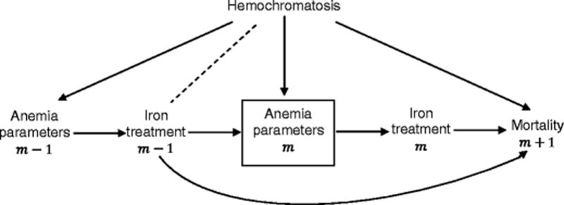
Standard regression methods include time-dependent anemia parameters m in the model, resulting in a biased estimate of the causal effect of iron treatment m − 1 on mortality due to an induced association with unmeasured hemochromatosis.
Section 2. A primer on the parametric g-formula and IPW for pharmacoepidemiologists
Unlike standard outcome regression approaches that condition on time-varying treatment and confounders, the parametric g-formula and IPW methods may produce valid effect estimates of dynamic treatment strategies when time-varying confounders are affected by past treatment. Like standard regression, the validity of these estimates rests on several assumptions. Specifically, to link estimates obtained from these methods to causal effects of dynamic treatment strategies we require the following assumptions: (i) no unmeasured confounding (sometimes called exchangeability) [35], (ii) consistency [42], guaranteeing the strategies under consideration are well-defined, and (iii) positivity, guaranteeing that for each dynamic treatment strategy under consideration and within each confounder and treatment history observed in the data through follow-up time m, it is possible to also observe in the data a value of treatment at m consistent with that strategy for all m [20, 23, 43]. For example, positivity would be violated in the running example – “at the beginning of every 2-day follow-up interval m, if ferritin level < x ng/mL then give 100 mg of intravenous iron in that interval, otherwise give 25 mg” – for the intensive iron strategy x =1200 if no patient in the observational study with ferritin level at or below 1200 ng/mL in a given 2-day interval received 100 mg of iron in that interval.
Robins [3] showed that given the assumptions of exchangeability, consistency, and positivity, we can write the mean/risk/hazard of an outcome of interest by/in a given follow-up time had, contrary to fact, we implemented a specified dynamic treatment strategy from baseline through that time as a function of only measured study variables. This function is known as the g-formula. Causal effects of following one versus another strategy are in turn defined by contrasts (e.g. differences or ratios) in the g-formula indexed by these different specified strategies.
The g-formula indexed by a specified strategy is in general a high-dimensional function. The parametric g-formula and IPW estimators are two possible approaches to estimating this high-dimensional function under parametric model assumptions on features of the distribution of study variables to deal with the curse of dimensionality. The two methods differ by the components of this distribution that require parametric model assumptions [35]. When implemented for the same study question, using the same data set, and under the same untestable assumptions about confounding, these two approaches will only give different results due to model misspecification. When completely flexible models are used under both methods, as in low dimensional settings, the two approaches are equivalent.
Table 2 summarizes the relative strengths and limitations of the parametric g-formula and IPW. The g-formula can also be estimated via doubly robust methods. These are extensions of IPW estimators that rely only on correct specification of one of two sets of models (a treatment/censoring model or a series of nested outcome regression models) [43–48]. It is generally recommended to estimate the same effect using multiple approaches and to check the consistency of the results. Similar results across different methods suggest the absence of gross model misspecification. Formal goodness-of-fit tests have been proposed [49].
Table 2.
Comparing parametric g-formula to inverse probability weighting of marginal structural models
| Method | Parametric g-formula | Inverse probability weighting of marginal structural models |
|---|---|---|
| Advantages |
|
|
| Limitations |
|
|
In this section, we briefly introduce the parametric g-formula and IPW in the context of our running iron dosing strategies example and provide resources for learning more. For simplicity, we discuss these methods under the assumption of no missing data, no measurement error, and no competing risks.
Parametric g-formula
The parametric g-formula can be understood as an extension of standardization to the setting of time-varying treatments and confounders. When interest is in the effects of different sustained treatment strategies on cumulative risk by an end of follow-up as in our running example, the parametric g-formula deals with the curse of dimensionality by imposing parametric models on the probability of the outcome and the joint density of confounders at each time, both conditional on past time-varying treatment and confounders amongst those who are at risk of the outcome up to that time. Here we give a brief description of how this approach could be implemented for estimating the effect of the sustained dynamic intravenous iron dosing strategies x =1200 versus x =500 on mortality risk by a specified end of follow-up (e.g. 5 years) in a population of ESRD patients initiating dialysis using observational data.
Step 1 – Parametrically estimate: (a) the joint density of post-baseline confounders at each follow-up time (including anemia parameters) conditional on past iron treatment and confounders amongst those surviving to that time and (b) the probability of mortality at each follow-up time conditional on past iron treatment and confounders amongst those surviving to that time. In both (a) and (b), models can be fit separately for each time point or pooled over time depending on how much data are available at each time point.
Step 2 – Simulate: time-varying confounder and treatment histories under the specified dynamic strategy using the model coefficients from Step 1a. Specifically, for each 2-day followup time m = 0,1, …, M (with m = 0 baseline and M the end of follow-up) and for each of the i = 1,2, …, n values of the baseline covariates in the data (obtained from the n patients at baseline in the study sample), implement the following steps iteratively: (a) For m = 0, set the baseline covariates to the observed values in the data. For m > 0, simulate confounders at time m from the estimate of their joint density in Step 1a given past confounder and treatment history previously generated through m − 1; (b) Set treatment to the value it should take at time m under the specified dynamic strategy given the previously generated (or observed at m =0) treatment and confounders. For example, under the intensive iron dosing strategy x =1200, we would assign a patient with simulated ferritin level of 1300 ng/mL at time m to 25 mg of iron at time m; (c) Compute the probability of mortality at time m + 1 conditional on the previously generated treatment and confounders using the estimated model coefficients from Step 1b.
Step 3 – Compute the risk by end of follow-up under the specified strategy: For each of the i = 1,2, …, n simulated histories obtained in Step 2 (which were generated from the n observed patient values of baseline covariates in the data and the estimated regression coefficients from Step 1), combine the time-varying discrete-time hazard estimates computed in Step 2c to get an estimate of the cumulative risk given the ith generated history under the specified strategy using the complement of a Kaplan-Meier survival estimator. The final estimate of cumulative mortality risk had we implemented the specified dynamic strategy in the population is then the average of these n history-specific risks.
Steps 2 and 3 are repeated for each strategy x =1200 versus x =500 to construct relative risks (or differences). The 95% confidence intervals can be constructed by repeating the entire algorithm (beginning with the model fitting in Step 1) in B bootstrap samples of the original n patients. Applications of this approach to estimating the effects of dynamic treatment strategies can be found for several chronic clinical conditions (Table 1). To identify the presence of gross model misspecification, we can compare model-based estimates for covariates means over time and the outcome risk under no treatment intervention with their nonparametric observed counterparts in the data. The model-based estimated can be obtained by fitting an additional model for the distribution of treatment at each time given past measured confounders and treatment in Step 1 and assigning treatment in Step 2b as a random draw from this distribution [23].
Inverse probability weighted estimation
The parametric g-formula requires correct specification of the conditional probabilities of the outcome and time-varying covariates in all follow-up intervals. This approach may be particularly vulnerable to bias due to model misspecification when there are many time-varying covariates and/or the number of follow-up intervals is large. Further, some degree of model misspecification may be guaranteed when the null hypothesis of no treatment effect is true; a phenomenon known as the “g-null paradox” [50, 51]. IPW estimation is an alternative approach which may be more robust to model misspecification and is not subject to the g-null paradox. Here we give a brief description of how this approach could be implemented for our running example.
Step 1 – Define strategies and make copies: Create a new data set that consists of stacked copies of the original data set with one copy for each strategy of interest. Index each copy with a strategy. For our running example, we would create a new data set consisting of two copies of the original data, one indexed by strategy x = 1200 and one by x = 500.
Step 2 – Artificially censor observations for deviation: In the restructured data with copies created in Step 1, for all strategies x, artificially censor patients in the copy indexed by strategy x at the time when they first deviate from this strategy. For example, in the copy of the data indexed by the intensive strategy x = 1200, a patient who had previous data consistent with this strategy through m = 4 would be artificially censored at time m = 5 if ferritin level was below 1200 ng/mL and did not receive 100 mg of iron at that time. Alternatively, a patient in the same copy who had ferritin below 1200 ng/mL and did not receive 100 mg of iron at time m = 0 would be artificially censored at time m = 0.
Step 3 – Estimate weights: Create time-varying artificial censoring weights to adjust for potential selection bias introduced by artificial censoring for strategy deviation in Step 2. At time m, the weight for a patient in the copy for strategy x who has not been artificially censored by time m is defined as the product over all times up to m of the inverse probability of remaining uncensored through that time given the measured past. The weight at time m for a patient in that copy who has been artificially censored by time m is 0. In realistic high-dimensional settings, the denominator of the weights need to be estimated via a parametric model. These patient-time-specific censoring weights will remove the association between the time-varying confounders and artificial censoring provided this censoring model is correctly specified.
Step 4 – Compute the risk by end of follow-up under the specified strategy: Apply weights created in Step 3 to the stacked artificially censored data set of Step 2 and compute the time-varying discrete-time hazards of outcome in the data copy for strategy x. These can then be used to derive estimates of the 5-year mortality risk under each strategy x and the effect comparing x = 1200 versus x = 500 obtained by corresponding risk ratios or differences. As with the parametric g-formula, we can derive inferences by repeating the algorithm in B bootstrap samples. In this case, analytic formulas for the variance are also available [43].
In practice, few individuals may be following one of the two strategies under consideration in our observational data. We could leverage information from other individuals by imposing a MSM that smooths over all strategies as a function of x where x can take more values than just 1200 or 500 [14, 15, 17–21, 52–57]. However, in doing so, we require an additional assumption that the MSM is correctly specified. Table 1 lists a few selected applications of the IPW approach to estimating causal effects of dynamic treatment strategies.
IPW estimators are generally less stable than the parametric g-formula in the presence of near violations of the positivity assumption. In this case, the denominator of the weights can become very small and in turn generate large weights and imprecision. This may be a particular problem when the number of follow-up times is large and when the treatment is continuous as in our intravenous iron dosing example. For continuous treatments, modified questions that compare random dynamic strategies can produce more stable IPW estimates [58–60]. These are strategies under which treatment at time m is allowed more than one value given a particular covariate history; for example, the strategy “at the beginning of every 2-day follow-up interval m, if ferritin level < x ng/mL then give 100 mg of intravenous iron in that interval with probability 0.8, and 75 mg of intravenous iron with probability 0.2, otherwise give 25 mg of intravenous iron”. Examining the distribution of the weights for extreme values can help identify the presence of near-positivity violations with weight truncation an option for decreasing variance at the expense of bias [61]. Alternative diagnostics that rely on additional parametric assumptions have been given by Petersen et al [62] based on parametric bootstrapping.
Section 3. Application of g-methods in pharmacoepidemiology
Practical challenges for applications of g-methods in pharmacoepidemiologic research
Most of published examples of g-methods applications (Table 1) are based on data from prospective cohort studies. Few applications of g-methods exist in the pharmacoepidemiology literature [14–19]. One explanation is the lack of sufficient information on time-varying confounders, including vital signs, laboratory tests results, clinical characteristics, patient’s response to treatment, and adverse side effects of treatment, in databases commonly used in pharmacoepidemiologic studies, such as administrative claims databases [63].
Fortunately, supplemental data from other data sources are increasingly available and contain richer, more granular patient-level information [64–67]. Linkage between multiple data sources offers a more complete picture of the treatment history of a patient and allows assessment of long-term effects of dynamic treatment strategies. For example, for ESRD patients on chronic hemodialysis, linked clinical and administrative claims databases contain detailed longitudinal information on patients, including medication treatment, routine laboratory tests, and healthcare encounters. These data provide relevant information needed to assess the safety and effectiveness of different intravenous iron dosing strategies in hemodialysis patients.
The limited availability of or familiarity with analytical tools needed to implement the relatively complex algorithms we reviewed above might also deter researchers from applying these approaches in their research. Applications of these methods require different levels of user-customization. For the parametric g-formula, the algorithm can be implemented using a publicly available SAS macro with documentation [68]. For the IPW estimation approach, Steps 3 and 4 of the algorithm can be implemented using standard regression software that allows for weights, despite lack of automated algorithms for Steps 1 and 2. An R package, ltmle, implements IPW of MSMs and doubly robust estimation for time-varying dynamic strategies [69]. Some tutorials that describe these methods are currently available [22, 23, 70–73]. However, further development of more accessible training tools, specifically targeting pharmacoepidemiologic research, is warranted.
Special considerations for pharmacoepidemiologic research
Table 3 reviews key considerations before implementing g-methods in practice. See also Hernán and Robins [74] and Zhang et al [16]. In addition to these considerations, there are several issues unique to observational pharmacoepidemiologic studies relying on electronic healthcare databases.
Table 3.
Some considerations before applying g-methods for treatment effects estimation in pharmacoepidemiologic studies
| Study Question | Is your research question well-defined?
|
| Study variables | Can you draw causal diagrams to identify relations among variables?
|
| Data consideration | Do you have all the necessary information captured for your analysis?
|
For pedagogic purposes, our running examples of intravenous iron dosing strategies are over-simplified versions of the types of dynamic treatment strategies for iron supplementation in ESRD patients that clinicians consider in practice. First, dynamic strategies of interest typically depend on multiple biomarkers rather than just one; for example, in addition to ferritin level cutoffs for determining iron dose, physicians may want to understand optimal joint cutoffs for ferritin, hemoglobin, and transferrin saturation levels. Further, in practice, measurement of treatments and confounders may not occur at the same frequency (e.g. every 2 days). For example, iron dose is typically adjusted only once per month while ferritin level is measured every three months and hemoglobin every two weeks. Also, monitoring may not occur at the same frequency for all patients but may, itself, be a dynamic process depending on the patient’s evolving health status. In such cases, time-varying monitoring status is a time-varying covariate that must be explicitly accounted for in the analysis. How it is handled has implications for the precise strategy definition, assumptions about confounding control, and effect estimation [75]. In settings where the gap between subsequent clinic visits is not strongly related to a patient’s health status, structuring the data to align with the treatment decision points results in more tractable estimation algorithms [17, 76, 77].
It can be challenging to identify treatment strategies to compare a priori given the inherent complexity and variation in real-world clinical practice, which are only partially recorded in electronic healthcare databases. Choosing such strategies generally requires a combination of input from clinical experts but also exploration of the observational data to understand what questions can be realistically supported with that data [76]. We may start with constructing a list of treatment strategies that are of clinical interest and commonly used, and then identify in our data which treatment strategies are most frequently observed.
Furthermore, patients may change or dis-enroll from a health plan (or switch dialysis provider as in our running example), resulting in loss to follow-up. The presence of censoring adds little additional practical complexity to either estimation approach. For the parametric g-formula, models in Step 1 are simply restricted to those remaining uncensored through each follow-up time; For IPW, weights are multiplied by inverse probability of censoring (by loss to follow-up) weights. Regardless of analytic method, when censoring is present in the data, additional untestable assumptions are required for causal inference. Importantly, g-methods require less restrictive censoring assumptions than standard outcome regression in that they allow censoring at any time during the follow-up to depend on time-varying measured covariates that may be affected by past treatment [41].
Conclusions
Dynamic treatment strategies are ubiquitous in clinical practice. Appropriate methods, such as the g-methods, are required to estimate the effects of these complex treatment strategies. While it is not feasible to rely on randomized clinical trials to answer all clinical questions, we can conduct observational pharmacoepidemiologic research to estimate the effects of some dynamic treatment strategies, especially with the increasing availability of data sources that provide more complete longitudinal information and better training and understanding of the g-methods.
Acknowledgments
Support for this work was provided to Dr. Li through a Thomas O. Pyle Fellowship from the Harvard Medical School & Harvard Pilgrim Health Care Institute. Dr. Young is supported by a faculty grant from the Harvard Pilgrim Health Care Institute. Dr. Toh is partially supported by the National Institute of Biomedical Imaging and Bioengineering (U01EB023683).
Footnotes
Compliance with Ethical Standards
Conflict of Interest
Xiaojuan Li received support for this work through a Thomas O. Pyle Fellowship from the Harvard Medical School & Harvard Pilgrim Health Care Institute.
Jessica G. Young is supported by a faculty grant from the Harvard Pilgrim Health Care Institute.
Sengwee Toh is also supported by the National Institute of Biomedical Imaging and Bioengineering (U01EB023683).
Human and Animal Rights and Informed Consent
This article does not contain any studies with human or animal subjects performed by the authors.
References
Recently published papers of particular interest have been highlighted as:
• Of importance
•• Of major importance
- 1.Ray WA. Evaluating medication effects outside of clinical trials: new-user designs. Am J Epidemiol. 2003;158(9):915–20. doi: 10.1093/aje/kwg231. [DOI] [PubMed] [Google Scholar]
- 2.Johnson ES, Bartman BA, Briesacher BA, Fleming NS, Gerhard T, Kornegay CJ, et al. The incident user design in comparative effectiveness research. Pharmacoepidemiol Drug Saf. 2013;22(1):1–6. doi: 10.1002/pds.3334. [DOI] [PubMed] [Google Scholar]
- 3.Robins J. A new approach to causal inference in mortality studies with a sustained exposure period—application to the healthy worker survivor effect. Mathematical Modelling. 1986;7(9–12):1393–512. [Google Scholar]
- 4.Murphy SA, van der Laan MJ, Robins JM. Marginal mean models for dynamic regimes. J Am Stat Assoc. 2001;96(456):1410–23. doi: 10.1198/016214501753382327. [DOI] [PMC free article] [PubMed] [Google Scholar]
- 5.Macdougall IC, Bircher AJ, Eckardt K-U, Obrador GT, Pollock CA, Stenvinkel P, et al. Iron management in chronic kidney disease: conclusions from a “Kidney Disease: Improving Global Outcomes” (KDIGO) Controversies Conference. Kidney Int. 2016;89(1):28–39. doi: 10.1016/j.kint.2015.10.002. [DOI] [PubMed] [Google Scholar]
- 6.Kidney Disease: Improving Global Outcomes (KDIGO) Anemia Work Group. KDIGO clinical practice guideline for anemia in chronic kidney disease. Kidney Int Suppl. 2012;2:279–335. [Google Scholar]
- 7.Locatelli F, Bárány P, Covic A, De Francisco A, Del Vecchio L, Goldsmith D, et al. Kidney Disease: Improving Global Outcomes guidelines on anaemia management in chronic kidney disease: a European Renal Best Practice position statement. Nephrol Dial Transplant. 2013;28(6):1346–59. doi: 10.1093/ndt/gft033. [DOI] [PubMed] [Google Scholar]
- 8.Kliger AS, Foley RN, Goldfarb DS, Goldstein SL, Johansen K, Singh A, et al. KDOQI US commentary on the 2012 KDIGO clinical practice guideline for anemia in CKD. Am J Kidney Dis. 2013;62(5):849–59. doi: 10.1053/j.ajkd.2013.06.008. [DOI] [PubMed] [Google Scholar]
- 9.Moist LM, Troyanov S, White CT, Wazny LD, Wilson J-A, McFarlane P, et al. Canadian society of nephrology commentary on the 2012 KDIGO clinical practice guideline for anemia in CKD. Am J Kidney Dis. 2013;62(5):860–73. doi: 10.1053/j.ajkd.2013.08.001. [DOI] [PubMed] [Google Scholar]
- 10.Krishnan M, Weldon J, Wilson S, Goyhkman I, Van Wyck D. Effect of maintenance iron protocols on ESA dosing and anemia outcomes [Abstract 153] Am J Kidney Dis. 2011;57(4):B55. [Google Scholar]
- 11.Miskulin DC, Tangri N, Bandeen-Roche K, Zhou J, McDermott A, Meyer KB, et al. Developing Evidence to Inform Decisions about Effectiveness (DEcIDE) Network Patient Outcomes in End Stage Renal Disease Study Investigators: Intravenous iron exposure and mortality in patients on hemodialysis. Clin J Am Soc Nephrol. 2014;9(11):1930–9. doi: 10.2215/CJN.03370414. [DOI] [PMC free article] [PubMed] [Google Scholar]
- 12.Schiller B. Implementing an IV iron administration protocol within a dialysis organization. 2014 Available at http://www.nephrologynews.com/implementing-an-iv-iron-administration-protocol-within-a-dialysis-organization/. [PubMed]
- 13.Li X, Kshirsagar AV, Brookhart MA. Safety of intravenous iron in hemodialysis patients. Hemodial Int. 2017;21(Suppl 1):S93–103. doi: 10.1111/hdi.12558. [DOI] [PMC free article] [PubMed] [Google Scholar]
- 14•.Cotton CA, Heagerty PJ. Evaluating epoetin dosing strategies using observational longitudinal data. Ann Appl Stat. 2014;8(4):2356–77. Describes an IPW of MSM method to compare multiple dynamic treatment strategies using electronic healthcare databases. [Google Scholar]
- 15•.Zhang Y, Thamer M, Kaufman J, Cotter D, Hernán MA. Comparative effectiveness of two anemia management strategies for complex elderly dialysis patients. Medical care. 2014;52(Suppl 3):S132–9. doi: 10.1097/MLR.0b013e3182a53ca8. Describes an inverse probability weighting approach to compare multiple dynamic treatment strategies using electronic healthcare databases. [DOI] [PMC free article] [PubMed] [Google Scholar]
- 16•.Zhang Y, Young JG, Thamer M, Hernán MA. Comparing the effectiveness of dynamic treatment strategies using electronic health records: an application of the parametric g-formula to anemia management strategies. Health Serv Res. 2017 May 30; doi: 10.1111/1475-6773.12718. Describes a parametric g-formula approach to compare multiple dynamic treatment strategies using electronic healthcare databases. [DOI] [PMC free article] [PubMed] [Google Scholar]
- 17•.Li X. PhD Dissertation. Chapel Hill (NC): University of North Carolina at Chapel Hill; 2017. Comparative effectiveness of intravenous iron treatment protocols in hemodialysis patients: causal inference with dynamic treatment regimes. Describes an approach to identify dynamic treatment strategies that can be realistically supported with the data and an application of inverse probability weighting approach to compare multiple dynamic strategies using electronic healthcare databases. [Google Scholar]
- 18••.Neugebauer R, Fireman B, Roy JA, O’Connor PJ, Selby JV. Dynamic marginal structural modeling to evaluate the comparative effectiveness of more or less aggressive treatment intensification strategies in adults with type 2 diabetes. Pharmacoepidemiol Drug Saf. 2012;21:99–113. doi: 10.1002/pds.3253. Describes a dynamic MSM approach to compare multiple dynamic treatment strategies using electronic healthcare databases. [DOI] [PubMed] [Google Scholar]
- 19.Neugebauer R, Fireman B, Roy JA, O’Connor PJ. Impact of specific glucose-control strategies on microvascular and macrovascular outcomes in 58,000 a dults with type 2 diabetes. Diabetes Care. 2013 doi: 10.2337/dc12-2675. [DOI] [PMC free article] [PubMed] [Google Scholar]
- 20••.Cain LE, Robins JM, Lanoy E, Logan R, Costagliola D, Hernán MA. When to start treatment? A systematic approach to the comparison of dynamic regimes using observational data. Int J Biostat. 2010;6(2) doi: 10.2202/1557-4679.1212. Article 18. Describes an approach to compare dynamic strategies by emulating randomized trials using observational data and discusses some complications that arise in such practice. [DOI] [PMC free article] [PubMed] [Google Scholar]
- 21.Cain LE, Logan R, Robins JM, Sterne JAC, Sabin C, et al. on behalf of The HIV-CAUSAL Collaboration When to initiate combined antiretroviral therapy to reduce rates of mortality and AIDS in HIV-infected individuals in developed countries. Ann Intern Med. 2011;154(8):509–15. doi: 10.1059/0003-4819-154-8-201104190-00001. [DOI] [PMC free article] [PubMed] [Google Scholar]
- 22••.Hernán MA, Lanoy E, Costagliola D, Robins JM. Comparison of dynamic treatment regimes via inverse probability weighting. Basic Clin Pharmacol Toxicol. 2006;98(3):237–42. doi: 10.1111/j.1742-7843.2006.pto_329.x. Describes a simple inverse probability weighting approach to compare two dynamic treatment strategies. [DOI] [PubMed] [Google Scholar]
- 23••.Young JG, Cain LE, Robins JM, O’Reilly EJ, Hernán MA. Comparative effectiveness of dynamic treatment regimes: an application of the parametric g-formula. Stat Biosci. 2011;3(1):119–43. doi: 10.1007/s12561-011-9040-7. Describes a parametric g-formula approach to compare dynamic treatment strategies. [DOI] [PMC free article] [PubMed] [Google Scholar]
- 24.Toh S, Hernández-Diaz S, Logan R, Robins JM, Hernán MA. Estimating absolute risks in the presence of nonadherence: an application to a follow-up study with baseline randomization. Epidemiology. 2010;21(4):528–39. doi: 10.1097/EDE.0b013e3181df1b69. [DOI] [PMC free article] [PubMed] [Google Scholar]
- 25.Wang L, Rotnitzky A, Lin X, Millikan RE, Thall PF. Evaluation of viable dynamic treatment regimes in a sequentially randomized trial of advanced prostate cancer. J Am Stat Assoc. 2012;107(498):493–508. doi: 10.1080/01621459.2011.641416. [DOI] [PMC free article] [PubMed] [Google Scholar]
- 26.Akdemir G, Markusse IM, Dirven L, Riyazi N, Steup-Beekman GM, Kerstens PJSM, et al. Effectiveness of four dynamic treatment strategies in patients with anticitrullinated protein antibody-negative rheumatoid arthritis: a randomised trial. RMD Open. 2016;2:e000143. doi: 10.1136/rmdopen-2015-000143.. [DOI] [PMC free article] [PubMed] [Google Scholar]
- 27.Robins JM, Hernán MA, Siebert U. Effects of multiple interventions In: Ezzati M; Lopez AD; Rodgers A; Murray CJL, editors Comparative Quantification of Health Risks: Global and Regional Burden of Disease Attributable to Selected Major Risk Factors. Geneva: World Health Organization; 2004. [Google Scholar]
- 28.Taubman SL, Robins JM, Mittleman MA, Hernán MA. Intervening on risk factors for coronary heart disease: an application of the parametric g-formula. Int J Epidemiol. 2009;38(6):1599–611. doi: 10.1093/ije/dyp192. [DOI] [PMC free article] [PubMed] [Google Scholar]
- 29.Lajous M, Willett WC, Robins J, Young JG, Rimm E, Mozaffarian D, et al. Changes in fish consumption in midlife and the risk of coronary heart disease in men and women. Am J Epidemiol. 2013;178(3):382–91. doi: 10.1093/aje/kws478. [DOI] [PMC free article] [PubMed] [Google Scholar]
- 30.Danaei G, Pan A, Hu FB, Hernán MA. Hypothetical lifestyle interventions in middle-aged women and risk of type 2 diabetes: a 24-year prospective study. Epidemiology. 2013;24:122–128. doi: 10.1097/EDE.0b013e318276c98a. [DOI] [PMC free article] [PubMed] [Google Scholar]
- 31.García-Aymerich J, Varraso R, Danaei G, Camargo CA, Hernán MA. Incidence of adult-onset asthma after hypothetical interventions on body mass index and physical activity: an application of the parametric g-formula. Am J Epidemiol. 2014;179(1):20–6. doi: 10.1093/aje/kwt229. [DOI] [PMC free article] [PubMed] [Google Scholar]
- 32.Jain P, Danaei G, Robins JM, Manson JE, Hernán MA. Smoking cessation and long-term weight gain in the Framingham Heart Study: an application of the parametric g-formula for a continuous outcome. Eur J Epidemiol. 2016;31(12):1223–9. doi: 10.1007/s10654-016-0200-4. [DOI] [PMC free article] [PubMed] [Google Scholar]
- 33.Wagner EH, Austin BT, Davis C, Hindmarsh M, Schaefer J, Bonomi A. Improving chronic illness care: translating evidence into action. Health Aff. 2001;20(6):64–78. doi: 10.1377/hlthaff.20.6.64. [DOI] [PubMed] [Google Scholar]
- 34.Robins J. A graphical approach to the identification and estimation of causal parameters in mortality studies with sustained exposure periods. J Chronic Dis. 1987;40(Suppl 2):S139–61. doi: 10.1016/s0021-9681(87)80018-8. [DOI] [PubMed] [Google Scholar]
- 35••.Robins JM, Hernán MA. Estimation of the causal effects of time-varying exposures. In: Fitzmaurice G, Davidian M, Verbeke G, Molenberghs G, editors. Longitudinal Data Analysis. Chapman and Hall CRC Press; New York: 2009. pp. 553–99. Introduces dynamic treatment strategies and methods to estimating effects of these strategies using observational data. [Google Scholar]
- 36.Robins JM, Hernán MA, Brumback B. Marginal structural models and causal inference in epidemiology. Epidemiology. 2000;11(5):550–60. doi: 10.1097/00001648-200009000-00011. [DOI] [PubMed] [Google Scholar]
- 37.Hernán MA, Brumback B, Robins JM. Marginal structural models to estimate the causal effect of zidovudine on the survival of HIV-positive men. Epidemiology. 2000;11(5):561–70. doi: 10.1097/00001648-200009000-00012. [DOI] [PubMed] [Google Scholar]
- 38.Robins JM. Marginal structural models, 1997 proceedings of the American Statistical Association, Section on Bayesian Statistical Science. Alexandria: VA American Statistical Association; 1998. pp. 1–10. [Google Scholar]
- 39.Pearl J. Causal diagrams for empirical research. Biometrika. 1995;82(4):669–88. [Google Scholar]
- 40.Pearl J. Causality: models, reasoning, and inference. 2nd. Cambridge University Press; New York: 2009. [Google Scholar]
- 41.Hernán MA, Hernández-Díaz S, Robins JM. A structural approach to selection bias. Epidemiology. 2004;15(5):615–25. doi: 10.1097/01.ede.0000135174.63482.43. [DOI] [PubMed] [Google Scholar]
- 42.VanderWeele TJ. Concerning the consistency assumption in causal inference. Epidemiology. 2009;20(6):880–3. doi: 10.1097/EDE.0b013e3181bd5638. [DOI] [PubMed] [Google Scholar]
- 43.Orellana L, Rotnitzky A, Robins JM. Dynamic regime marginal structural mean models for estimation of optimal dynamic treatment regimes, Part I: Main content. Int J Biostat. 2010;6(2) Article 8. [PubMed] [Google Scholar]
- 44.Bang H, Robins JM. Doubly robust estimation in missing data and causal inference models. Biometrics. 2005;61(4):962–73. doi: 10.1111/j.1541-0420.2005.00377.x. [DOI] [PubMed] [Google Scholar]
- 45.van der Laan MJ. Targeted maximum likelihood based causal inference: Part I. Int J Biostat. 2010;6(2) doi: 10.2202/1557-4679.1211. Article 2. [DOI] [PMC free article] [PubMed] [Google Scholar]
- 46.van der Laan MJ. Targeted maximum likelihood based causal inference: Part II. Int J Biostat. 2010;6(2) doi: 10.2202/1557-4679.1211. Article 3. [DOI] [PMC free article] [PubMed] [Google Scholar]
- 47.van der Laan MJ, Gruber S. Targeted minimum loss based estimation of causal effects of multiple time point interventions. Int J Biostat. 2012;8(1) doi: 10.1515/1557-4679.1370. Article 9. [DOI] [PubMed] [Google Scholar]
- 48•.Petersen M, Schwab J, Gruber S, Blaser N, Schomaker M, van der Laan M. Targeted maximum likelihood estimation for dynamic and static longitudinal marginal structural working models. J Causal Inference. 2014;2(2):147–85. doi: 10.1515/jci-2013-0007. Describes how to estimate marginal structural models for dynamic treatment strategies using doubly-robust methods. [DOI] [PMC free article] [PubMed] [Google Scholar]
- 49.Robins JM, Rotnitzky A. Comment on the Bickel and Kwon article, “Inference for semiparametric models: Some questions and an answer”. Statistica Sinica. 2001;11(4):920–36. [“On double robustness”] [Google Scholar]
- 50.Robins JM, Wasserman L. Estimation of effects of sequential treatments by reparameterizing directed acyclic graphs. In: Geiger D, Shenoy P, editors. Proceedings of the Thirteenth Conference on Uncertainty in Artificial Intelligence, Providence Rhode Island. San Francisco: Morgan Kaufmann: 1997. pp. 409–20. [Google Scholar]
- 51.Young JG, Tchetgen Tchetgen EJ. Simulation from a known Cox MSM using standard parametric models for the g-formula. Stat Med. 2014;33(6):1001–14. doi: 10.1002/sim.5994. [DOI] [PMC free article] [PubMed] [Google Scholar]
- 52.Orellana L, Rotnitzky A, Robins JM. Dynamic regime marginal structural mean models for estimation of optimal dynamic treatment regimes, Part II: Proofs and Additional Results. Int J Biostat. 2010;6 doi: 10.2202/1557-4679.1242. Article 8. [DOI] [PMC free article] [PubMed] [Google Scholar]
- 53.van der Laan MJ, Petersen ML. Causal effect models for realistic individualized treatment and intention to treat rules. Int J Biostat. 2007;3(1) doi: 10.2202/1557-4679.1022. Article 3. [DOI] [PMC free article] [PubMed] [Google Scholar]
- 54.Robins J, Orellana L, Rotnitzky A. Estimation and extrapolation of optimal treatment and testing strategies. Stat Med. 2008;27(23):4678–721. doi: 10.1002/sim.3301. [DOI] [PubMed] [Google Scholar]
- 55.Cotton CA, Heagerty PJ. A data augmentation method for estimating the causal effect of adherence to treatment regimens targeting control of an intermediate measure. Stat Biosci. 2011;3(1):28–44. [Google Scholar]
- 56.Shortreed SM, Moodie EEM. Estimating the optimal dynamic antipsychotic treatment regime: Evidence from the sequential multiple-assignment randomized clinical antipsychotic trials of intervention and effectiveness schizophrenia study. J R Stat Soc Ser C Appl Stat. 2012;61(4):577–99. doi: 10.1111/j.1467-9876.2012.01041.x. [DOI] [PMC free article] [PubMed] [Google Scholar]
- 57.Orellana L, Rotnitzky AG, Robins JM. Generalized marginal structural models for estimating optimal treatment regimes Technical Report, Department of Biostatistics. Harvard School of Public Health; 2006. [Google Scholar]
- 58.Munoz ID, van der Laan M. Population intervention causal effects based on stochastic interventions. Biometrics. 2012;68(2):541–9. doi: 10.1111/j.1541-0420.2011.01685.x. [DOI] [PMC free article] [PubMed] [Google Scholar]
- 59.Haneuse S, Rotnitzky A. Estimation of the effect of interventions that modify the received treatment. Statistics in Medicine. 2013;32(30):5260–77. doi: 10.1002/sim.5907. [DOI] [PubMed] [Google Scholar]
- 60.Young JG, Hernán MA, Robins JM. Identification, estimation and approximation of risk under interventions that depend on the natural value of treatment using observational data. Epidemiologic methods. 2014;3(1):1–19. doi: 10.1515/em-2012-0001. [DOI] [PMC free article] [PubMed] [Google Scholar]
- 61.Cole SR, Hernán MA. Constructing inverse probability weights for marginal structural models. Am J Epidemiol. 2008;168(6):656–64. doi: 10.1093/aje/kwn164. [DOI] [PMC free article] [PubMed] [Google Scholar]
- 62.Petersen ML, Porter KE, Gruber S, Wang Y, van der Laan MJ. Diagnosing and responding to violations in the positivity assumption. Stat Methods Med Res. 2012;21(1):31–54. doi: 10.1177/0962280210386207. [DOI] [PMC free article] [PubMed] [Google Scholar]
- 63.Schneeweiss S, Avorn J. A review of uses of health care utilization databases for epidemiologic research on therapeutics. J Clin Epidemiol. 2005;58(4):323–37. doi: 10.1016/j.jclinepi.2004.10.012. [DOI] [PubMed] [Google Scholar]
- 64.Murray MD. Use of Data from Electronic Health Records for Pharmacoepidemiology. Current Epidemiology Reports. 2014;1(4):186–93. [Google Scholar]
- 65.Foley RN, Collins AJ. The USRDS: what you need to know about what it can and can’t tell us about ESRD. Clin J Am Soc Nephrol. 2013;8(5):845–51. doi: 10.2215/CJN.06840712. [DOI] [PubMed] [Google Scholar]
- 66.Schmidt M, Schmidt SA, Sandegaard JL, Ehrenstein V, Pedersen L, Sorensen HT. The Danish National Patient Registry: a review of content, data quality, and research potential. Clin Epidemiol. 2015;7:449–90. doi: 10.2147/CLEP.S91125. [DOI] [PMC free article] [PubMed] [Google Scholar]
- 67.Andrade SE, Berard A, Nordeng HME, Wood ME, van Gelder MMHJ, Toh S. Administrative claims data versus augmented pregnancy data for the study of pharmaceutical treatments in pregnancy. Curr Epidemiol Rep. 2017;4(2):106–16. doi: 10.1007/s40471-017-0104-1. [DOI] [PMC free article] [PubMed] [Google Scholar]
- 68.Logan RW, Young JG, Taubman S, Lodi S, Picciotto S, Danaei G, et al. The GFORMULA SAS macro. 2017 https://www.hsph.harvard.edu/causal/software./
- 69.Lendle, Samuel, Schwab, Joshua, Petersen, Maya, van der Laan, Mark J. ltmle: An R Pack-age Implementing Targeted Minimum Loss-based Estimation for Longitudinal Data [Google Scholar]
- 70.Daniel RM, De Stavola BL, Cousens SN. gformula: Estimating causal effects in the presence of time-varying confounding or mediation using the g-computation formula. Stata Journal. 2011;11(4):479–517. [Google Scholar]
- 71••.Daniel RM, Cousens SN, De Stavola BL, Kenward MG, Sterne JAC. Methods for dealing with time-dependent confounding. Stat Med. 2013;32(9):1584–618. doi: 10.1002/sim.5686. Tutorial for g-methods. [DOI] [PubMed] [Google Scholar]
- 72••.Causal Inference Methods for PCOR using Observational Data Conference. CIMPODS. 2017 Retrieved from http://www.cimpod2017.org. Includes tutorials on g-methods for dynamic treatment strategies.
- 73••.Comparative Effectiveness Research Based on Observational Data to Emulate a Target Trial (CERBOT) Retrieved from http://cerbot.org/. Includes tutorials on g-methods for dynamic treatment strategies.
- 74••.Hernán MA, Robins JM. Using big data to emulate a target trial when a randomized trial is not available. Am J Epidemiol. 2016;183(8):758–64. doi: 10.1093/aje/kwv254. Outlines a framework to obtain causal effect in comparative effectiveness research using observational data. [DOI] [PMC free article] [PubMed] [Google Scholar]
- 75.Hernán MA, McAdams M, McGrath N, Lanoy E, Costagliola D. Observation plans in longitudinal studies with time-varying treatments. Stat Methods Med Res. 2009;18(1):27–52. doi: 10.1177/0962280208092345. [DOI] [PMC free article] [PubMed] [Google Scholar]
- 76.Li X, Cole SR, Kshirsagar AV, Fine J, Stürmer T, Brookhart MA. Identification of dynamic treatment regimes in complex longitudinal data. [unpublished, revise & resubmit] [Google Scholar]
- 77.Brookhart MA. Counterpoint: the treatment decision design. Am J Epidemiol. 2015;182(10):840–5. doi: 10.1093/aje/kwv214. [DOI] [PMC free article] [PubMed] [Google Scholar]