Low-Dose Dynamic Cerebral Perfusion Computed Tomography Reconstruction via Kronecker-Basis Representation Tensor Sparsity Regularization

Abstract

Dynamic cerebral perfusion computed tomography (DCPCT) has the ability to evaluate the hemodynamic information throughout the brain. However, due to multiple 3-D image volume acquisitions protocol, DCPCT scanning imposes high radiation dose on the patients with growing concerns. To address this issue, in this paper, based on the robust principal component analysis (RPCA, or equivalently the low-rank and sparsity decomposition) model and the DCPCT imaging procedure, we propose a new DCPCT image reconstruction algorithm to improve low dose DCPCT and perfusion maps quality via using a powerful measure, called Kronecker-basis-representation tensor sparsity regularization, for measuring low-rankness extent of a tensor. For simplicity, the first proposed model is termed tensor-based RPCA (T-RPCA). Specifically, the T-RPCA model views the DCPCT sequential images as a mixture of low-rank, sparse, and noise components to describe the maximum temporal coherence of spatial structure among phases in a tensor framework intrinsically. Moreover, the low-rank component corresponds to the “background” part with spatial–temporal correlations, e.g., static anatomical contribution, which is stationary over time about structure, and the sparse component represents the time-varying component with spatial–temporal continuity, e.g., dynamic perfusion enhanced information, which is approximately sparse over time. Furthermore, an improved nonlocal patch-based T-RPCA (NL-T-RPCA) model which describes the 3-D block groups of the “background” in a tensor is also proposed. The NL-T-RPCA model utilizes the intrinsic characteristics underlying the DCPCT images, i.e., nonlocal self-similarity and global correlation. Two efficient algorithms using alternating direction method of multipliers are developed to solve the proposed T-RPCA and NL-T-RPCA models, respectively. Extensive experiments with a digital brain perfusion phantom, preclinical monkey data, and clinical patient data clearly demonstrate that the two proposed models can achieve more gains than the existing popular algorithms in terms of both quantitative and visual quality evaluations from low-dose acquisitions, especially as low as 20 mAs.

I. INTRODUCTION

Dynamic cerebral perfusion computed tomography (DCPCT) imaging is a promising tool for acute stroke evaluation because DCPCT can visualize and quantify hemodynamic information of tissue and vessels [1]. In clinics, after bolus injection of a contrast agent, continuous scans of the brain in cine mode are performed, then using the acquired sequential enhanced images, the contrast intake curves (or equivalently, time density curves, TDCs) can be estimated. And according to central volume principle, the physiological data, which is typically displayed in perfusion maps, including cerebral blood flow (CBF), cerebral blood volume (CBV), and mean transit time (MTT), can be derived from the contrast intake curves [1]. However, because of multiple three-dimensional image volume acquisitions, DCPCT imaging imposes high radiation dose on the patients, which might increase the underlying risk of cancer [2]. Based on as low as reasonably achievable (ALARA) principle, the benefit versus-harm ratio should be carefully assessed for all cases and excessive radiation dose should be reduced. Therefore, minimizing the radiation dose in DCPCT imaging is a useful and interesting topic with ongoing research activities.

In general, there are two representative approaches to reduce the radiation dose in DCPCT imaging, i.e., reducing tube current and/or decreasing the number of projections [2]. However, the associated DCPCT images from current standard filtered back-projection (FBP) reconstruction algorithm would be degraded by unavoidable noise-induced artifacts, which could also influence the perfusion maps calculation accuracy. To address this issue, many dedicated DCPCT imaging methods have been proposed [3]–[17]. For example, one major category is to directly reduce the noise of DCPCT image reconstructed by the FBP algorithm, including the edge preserving spatial-temporal filters such as the anisotropic diffusion filter [3], the bilateral filter [4] and the non-local means filter [5], and the spatial-temporal filters such as the highly constrained back projection (HYPR) filter [6] and the multiband filter (MBF), followed by the standard deconvolution algorithms, such as the singular value decomposition (SVD)-based algorithms [18]. These methods have shown a good capability to suppress both the noise of DCPCT images and perfusion maps to some extent, but they might result in spatial resolution loss because the noise in DCPCT is non-uniform and the SVD-based deconvolution algorithms are also sensitive to the noise [19]. Another major category is to combine the stable deconvolution procedure with image noise suppression procedures in perfusion maps estimation, such as the spatial-temporal model [7], Bayesian probabilistic frame work [8], online dictionary learning approach [9], and total variation (TV)-based regularization [10], [11]. The phantom and patient studies demonstrated the ability of these methods on improving the residue functions estimation accuracy as well as the perfusion maps quality. Last major category is to obtain the high quality DCPCT images via the statistical iterative reconstruction (SIR) methods, and then the desired perfusion maps are estimated from these images via the existing deconvolution algorithms [12]–[17]. These methods have the capabilities of suppressing noise-induced artifacts in the desired images because the SIR methods incorporate both accurate CT system modelling and statistics modelling of projection measurements. Thus, high quality CT image reconstruction and robust perfusion maps estimation via the SIR method are one of the most potential strategies for low-dose DCPCT imaging.

In this study, according to the robust principal component analysis (RPCA, or equivalently the low-rank plus sparsity decomposition) [20] and the DCPCT imaging procedure, we propose a new DCPCT image reconstruction algorithm to improve low-dose DCPCT images and perfusion maps quality via using a powerful regularization, called Kronecker-basis representation (KBR) tensor sparsity measure, for representing low-rank essence of a tensor. This measure has been very recently proposed, and been substantiated to be effective in multiple applications in computer vision. Similar to the RPCA model, the proposed model views the DCPCT sequential images as a mixture of low-rank and sparse components to describe the maximum temporal coherence of spatial structure among phases in a tensor framework intrinsically. For simplicity, the new model is called as the tensor-based RPCA (T-RPCA) model. Specifically, the low-rank component corresponds to the “background” with spatial-temporal correlations, e.g. static anatomical contribution, which is stationary over time about structure, and the sparse component represents the time-varying component with spatial-temporal continuity, e.g. dynamic perfusion enhanced information, which is approximately sparse over time [20], [21]. In the T-RPCA model, the tensor-based decomposition (i.e., Tucker decomposition [22] and CANDE-COMP/PARAFAC (CP) decomposition [23]) operator is utilized to describe “background” part of DCPCT image and the tensor total variation (TTV) is utilized to regularize the dynamic perfusion information in the DCPCT image. Furthermore, an improved nonlocal patch-based T-RPCA (NL-T-RPCA) model which describes the 3D block groups of the “background” in a tensor is also proposed. The NL-T-RPCA model utilizes the intrinsic characteristics underlying the DCPCT images, i.e., nonlocal self-similarity and global correlation. Moreover, we present two effective iterative algorithms for the two models with a robust convergence result, respectively. In addition, we study the performance of two proposed algorithms on a digital brain perfusion phantom, preclinical monkey data and patient data in low-dose cases, especially as low as 20 mAs.

II. METHODS AND MATERIALS

A. DCPCT Imaging Model

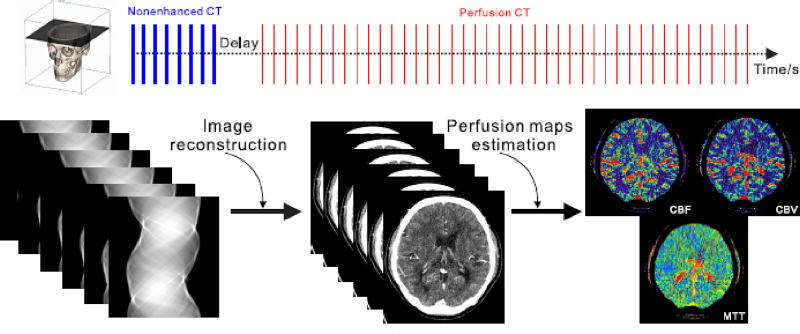
As shown in Fig. 1, the DCPCT image volume can be viewed as a 4-order tensor where first three dimensions are about spatial and the forth dimension is about time. For simplicity, only a desired 3-order DCPCT object with T frames 𝒳 ∈ ℝ^{I₁×I₂×I₃} (𝒳 = {x_i, i ≤ T}) where x_i represents the i-th two dimensional frame of the DCPCT images) is utilized. Without loss of generality, the relationship between the available 3-order DCPCT projection data y and the desired 3-order DCPCT images X can be expressed as follows:

$$𝒴=\{y_i=A_i{x}_i+N_i\le T\},$$ (1)

where A_i denotes the system matrix and is assumed to be independent of the index i. N_i denotes the noise disturbance. In this study, the goal of DCPCT images reconstruction is to estimate the desired 3D DCPCT images X from the measured projections y via penalized weighted least-squares (PWLS) objective function, i.e.,

$${𝒳}^{\ast }=\underset{𝒳}{\text{arg min}}{\Vert 𝒴-A𝒳\Vert }_W^2+\beta R(𝒳),$$ (2)

where A represents a linear operator composed of system matrices {A_i}. W = diag{W_i}, 1 ≤ i ≤ T denotes the weighting matrix. W_i is the diagonal weighting matrix at the i-th frame and can be defined as $W_i={\sum }_i^{-1}$, and ${\sum }_i^{-1}$ is a diagonal matrix. ${\sigma }_{i,k}^2$ is the element in the ${\sum }_i^{-1}$, representing the variance of the projection measurement y_i at detector bin k. In this study, the variance ${\sigma }_{i,k}^2$ is determined based on our previous research [24].

Fig. 1.

Illustration of the DCPCT imaging procedure.

In Eq. (2), R(𝒳) denotes the penalty term which has the ability to integrate prior information in image reconstruction procedure. β is the penalty weight which controls the optimal solution of Eq. (2). In this study, the major contribution is to introduce two new spatial-temporal models from the tensor perspective. The description of the two models will be discussed in Sec. II-B.

B. Tensor-Based RPCA Models

It is noted that the low-rank component of a 3D CT image tensor corresponds to the “background” with spatial-temporal correlations, e.g. static anatomical contribution, which is stationary over time about structure and its sparse component represents the time-varying component with spatial-temporal continuity, e.g. dynamic perfusion information, which is approximately sparse over time [20], [21]. Motivated by these observations, the 3-order tensor 𝒳 can be intrinsically composed of low-rank component ℬ (i.e., the ideal static anatomical contribution), sparse component ℱ (i.e., the dynamic perfusion enhanced information) and noise disturbance N, which is defined as follows:

$$𝒳=ℬ+ℱ+𝒩.$$ (3)

Accordingly, the DCPCT image reconstruction model can be defined as follows:

$$\underset{X,B,F,N}{\text{min}}\lambda {\mathrm{\Omega }}_1(ℱ)+{\mathrm{\Omega }}_2(ℬ)+\gamma {\mathrm{\Omega }}_3(𝒩)$$ (4)

$$s.t.𝒳=ℬ+ℱ+𝒩,𝒴=A𝒳,$$

where λ and γ are the penalty weights. Ω₁(ℱ), Ω₂(ℬ) and Ω₃(𝒩) denote the penalty terms regularizing the prior information of the dynamic perfusion changes, static anatomical contribution and noise disturbance, respectively. Generally for the noise disturbance 𝒩, Ω₃(𝒩) is specified as $\frac{1}{2}{\Vert 𝒩\Vert }_F^2$ where ‖·‖_F denotes the Frobenius norm. Because the dynamic perfusion information is different and sparse over time, the tensor-based total variation (TTV) regularization [10] is introduced to model the ℱ, which can be defined as follows:

$${\mathrm{\Omega }}_1(ℱ)={\Vert ℱ\Vert }_{\mathit{\text{TTV}}}={\Vert \nabla ℱ\Vert }_1,$$ (5)

where ∇ is the forward finite difference operator. ‖·‖₁ denotes the l₁ norm. As the static anatomical contribution is temporally correlated, in 2011, Gao et al. characterized the static anatomical component as low-rank matrix mathematically and utilized nuclear norm to penalize the rank of the specific matrix [20]. However, the low-rank formulation neglects the structure information among spatial dimension. One of the promising solutions is to utilize the tensor properties in the static anatomical component ℬ [21], [25]. In this study, two tensor-based models are introduced to describe the static anatomical component ℬ, i.e., Tensor-based regularization model and Nonlocal Tensor-based regularization model

1) Tensor-Based Regularization Model

Because both Tucker decomposition [22] and CP decomposition [23] contain insightful tensor sparsity, by integrating rational sparsity understanding elements from both decomposition forms, the low-rankness characteristic of the static anatomical component ℬ can be constructed by a powerful KBR measure, for measuring low-rankness extent of a tensor, which is proposed in [25]:

$${\mathrm{\Omega }}_2(ℬ)={\Vert 𝒞\Vert }_0+\zeta \prod _{i=1}^3\mathit{\text{rank}}(B_{(i)}),$$ (6)

where 𝒞 denotes the core tensor of ℬ in the Tucker decomposition. B_(i) represents the mode-i (1 ≤ i ≤ 3) unfolding matrix, and ζ is the penalty parameter controlling the tradeoff between two terms B_(i) = unfold_i(ℬ). ‖·‖₀ denotes the l₀ norm. Compared with the conventional low-rank matrix model, the tensor-based regularization model fully introduces the spatial and temporal correlations within the static anatomical component ℬ. In addition, it is noted that the R(ℬ) in Eq. (6) takes both intrinsic sparsity existing in Tucker and CP decompositions into consideration, i.e., the first term constrains the number of Kronecker bases that describe the static anatomical component ℬ, and the second term physically represents the size of core tensor in the Tucker decomposition by penalizing the low-rank property along each tensor mode [25].

Therefore, by integrating the modeling of the dynamic perfusion changes Ω₁(ℱ), static anatomical contribution Ω₂(ℬ) in Eq. (6) and noise disturbance Ω₃(𝒩), the objective function in Eq. (4) can be written as follows:

$$\underset{𝒳,ℬ,ℱ,{𝒩}_{B_{(i)}},𝒞}{\text{min}}{\Vert \nabla ℱ\Vert }_1+{\Vert 𝒞\Vert }_0+\zeta \prod _3^3\mathit{\text{rank}}(B_{(i)})+\frac{\gamma }{2}{\Vert 𝒩\Vert }_F^2,$$ (7)

$$s.t.𝒳=ℬ+ℱ+𝒩,𝒴=A𝒳,$$

the model is referred as Tensor-based RPCA (T-RPCA) in the following sections.

2) Nonlocal Tensor-Based Regularization Model

It is noted that the use of image nonlocal (NL) self-similarity prior, referring to the fact that a local patch often exists many nonlocal similar patches to it across the image, has significantly enhance the processing performance [5], [26]. In general, the patch-based strategies applied on the 2D matrix can be extended to 3-order tensor. For a 3-order tensor patch ${𝒫}_1^1\in {ℝ}^{s_m\times s_n\times s_t}$, we can find a collection of 3-order tensor ${𝒫}_1^p\in {ℝ}^{s_m\times s_n\times s_t}$, (2 ≤ p ≤ P + 1) where P denotes the number of the similar patches) similar to ${𝒫}_1^1\in {ℝ}^{s_m\times s_n\times s_t}$, across the static anatomical component ℬ via K-nearest neighbor method after static anatomical contribution ℬ is segmented into many overlapped 3D patches and then cluster them into a 4-order tensor C𝒫_i which can defined as follows:

$$C{𝒫}_1=\left(\begin{array}{c}{𝒫}_1^1\hfill \\ {𝒫}_1^2\hfill \\ \dots \hfill \\ {𝒫}_1^{p+1}\hfill \end{array}\right),$$ (8)

Where C represents the operation that first extract all 3-order tensor patches similar to the selected one and then cluster the selected patch and all 3-order similar tensor patches into a 4-order tensor. Therefore, the static anatomical component B can be penalized as follows:

$${\mathrm{\Omega }}_2(ℬ)=\sum _{i=1}^{K}R(C{𝒫}_i),$$ (9)

where R(C𝒫_i) reflects the priori knowledge of the i–th 4-order tensor C𝒫_i. More details are listed in our supplementary material.

Therefore, by integrating the modeling of the dynamic perfusion changes Ω₁(ℱ) same to these in the T-RPCA model, static anatomical contribution Ω₂(ℬ) in Eq. (9) and noise disturbance Ω₃(𝒩), the objective function in Eq. (4) can be written as follows:

$$\underset{𝒳,ℬ,ℱ,𝒩𝒞{𝒫}_i}{\text{min}}{\Vert \nabla ℱ\Vert }_1+\sum _{i=1}^{K}R(C{𝒫}_i)+\frac{\gamma }{2}{\Vert 𝒩\Vert }_F^2$$ (10)

$$s.t.𝒳=ℬ+ℱ+𝒩,𝒴=A𝒳,$$

the model is referred as Nonlocal-Tensor-based RPCA (NL-T-RPCA) in the following sections.

C. Optimization Approach

To minimize the objective function in Eq. (7), an alternating direction method of multipliers (ADMM) was specifically designe [27]. In particular, the T-RPCA model in Eq. (7) can be rewritten as follows:

$$\underset{𝒳,ℬ,ℱ,𝒩B_{(i)},𝒞,𝒢}{\text{min}}{\Vert 𝒢\Vert }_{1+}{\Vert 𝒞\Vert }_0+\zeta \prod _{i=1}^3\mathit{\text{rank}}(B_{(i)})+\frac{\gamma }{2}{\Vert 𝒞\times {}_1{U}_1\times {}_2{U}_2\times {}_3{U}_3+ℱ-𝒳\Vert }_F^2,$$ (11)

$$s.t.𝒴=A𝒳,$$

$$\nabla ℱ=𝒢,{(𝒞\times {}_1{U}_1\times {}_2{U}_2\times {}_3{U}_3)}_{(i)}=B_{(i),}$$

where the factor matrices U_i(i = 1,2,3) denote orthogonal in columns. It is noted that the objective function in Eq. (11) can be solved by its Lagrangian dual form. Then its augmented Lagrangian function can be written as follows:

$$L(𝒢,𝒞,B_{(i)},U_i,ℱ,𝒳)={\Vert 𝒢\Vert }_1+{\Vert 𝒞\Vert }_0+\zeta \prod _{i=1}^3\mathit{\text{rank}}(B_{(i)})+\frac{\gamma }{2}{\Vert 𝒞\times {}_1{U}_1\times {}_2{U}_2\times {}_3{U}_3+ℱ-𝒳\Vert }_F^2+\sum _i\langle 𝒞\times {}_1{U}_1\times {}_2{U}_2\times {}_3{U}_3-B_{(i)},{\mathrm{\Lambda }}_i^B\rangle +\sum _i\frac{{\eta }_i^B}{2}{\Vert 𝒞\times {}_1{U}_1\times {}_2{U}_2\times {}_3{U}_3-B_{(i)}\Vert }_F^2+\langle \nabla ℱ-𝒢,{\mathrm{\Lambda }}^{ℱ}\rangle +\frac{{\eta }^{ℱ}}{2}{\Vert \nabla ℱ-𝒢\Vert }_F^2+\langle 𝒴-A𝒳,{\mathrm{\Lambda }}^{𝒳}\rangle +\frac{{\eta }^{𝒳}}{2}{\Vert 𝒴-A𝒳\Vert }_F^2$$ (12)

where ${\mathrm{\Lambda }}_i^B$, Λ^ℬ and Λ^𝒳 are the Lagrange multipliers and ${\eta }_i^B$, η^ℱ and η^𝒳 are positive penalty scalars. The objective function in Eq. (12) can be solved with the ADMM framework, and the optimization sub-problem with respect to each variable can be solved by the following sub-problems:

1) 𝒳 Sub-Problem

With respect to 𝒳, the L(𝒢, 𝒞, B_(i), U_(i), ℱ, 𝒳) can be solved as follows:

$$(\gamma I+{\eta }^{𝒳}A\text{'}A)𝒳=\gamma (𝒞\times {}_1{U}_1\times {}_2{U}_2\times {}_3{U}_3+ℱ)+A\text{'}({\eta }^{𝒳}𝒴-{\mathrm{\Lambda }}^{𝒳}),$$ (13)

It is obvious that Eq. (13) can be solved by the conjugate gradient algorithm, and the corresponding solution can be written as follows:

$$𝒳=\frac{(I-\frac{{\eta }^{𝒳}}{\gamma +{\eta }^{𝒳}}A\text{'}A)}{\gamma }\times \frac{\gamma (𝒞\times {}_1{U}_1\times {}_2{U}_2\times {}_3{U}_3+ℱ)+A\text{'}({\eta }^{𝒳}Y-{\mathrm{\Lambda }}^{𝒳})}{\gamma }$$ (14)

2) 𝒞 and U_i Sub-Problems

With respect to 𝒞 and U_i (i = 1,2,3), the L(𝒢, 𝒞, B_(i), U_i, ℱ, 𝒳) can be solved as follows: (i)for 𝒞:

$$\underset{C}{\text{min}}\frac{1}{\gamma +3\mu }\mathit{\text{Fappro}}(𝒞)+\frac{1}{2}\Vert 𝒞\times {}_1{U}_1\times {}_2{U}_2\times {}_3{U}_3-{\frac{(\gamma (𝒳-ℱ)+\sum _i\mathit{\text{Fold}}({\eta }_i^B{B}_{(i)}-{\mathrm{\Lambda }}_{i}B))}{\gamma +3\mu }\Vert }_F^2$$ (15)

where $\mathit{\text{Fappro}}(𝒞)=\sum _{i_1,i_2,i_3}\text{log}(|c{i}_1,i_2,i_3|+\epsilon )$ is the log-sum norm of the vector, approximating the ‖𝒞‖₀ [28]. After multiplying mode-i $U_i^T$ on each mode, the solution of Eq. (15) can be written as follows:

$${𝒞}^{+}=R_{\frac{1}{\gamma +3\mu },\epsilon }(\frac{(\gamma (X-F)+\sum _i\mathit{\text{Fold}}({\eta }_i^B{B}_i-{\mathrm{\Lambda }}_i^B))}{\gamma +3\mu }\times {}_1{U}_1\times {}_2{U}_2\times {}_3{U}_3),$$ (16)

where $R_{{\tau }_1,{\tau }_2}(\omega )=\{\begin{array}{cc}0\hfill & \mathit{\text{if }}{\sigma }_2\le 0\hfill \\ \mathit{\text{sign}}(\omega )\left(\frac{{\sigma }_1+{\sigma }_2}{2}\right)\hfill & \mathit{\text{if }}{\sigma }_2>0\hfill \end{array}$ wherein σ₁=|ω|−τ₂ and σ₂ = (σ₁)² − 4(τ₁ − ε|ω|) [29].

(ii) for U_i : With respect to U_i, the L(𝒢, 𝒞, B_(i), U_i, ℱ, 𝒳) can be solved as follows:

$$\underset{U_1}{\text{min }}\frac{1}{2}{\Vert 𝒞\times {}_1{U}_1\times {}_2{U}_2\times {}_3{U}_3-\frac{(\gamma (𝒳-ℱ)+\sum _i\mathit{\text{Fold}}({\eta }_i^B{B}_{(i)}-{\mathrm{\Lambda }}_{i}B))}{\gamma +3\mu }\Vert }_F^2,$$ (17)

Then, Eq.(17) can be transformed into as follows:

$$\underset{U_1^T{U}_1=1}{\text{max }}\langle A_1,U_1\rangle ,$$

where

$$A_1=-{\left(\frac{(\gamma (𝒳-ℱ)+\sum _i\mathit{\text{Fold}}({\eta }_i^B{B}_{(i)}-{\mathrm{\Lambda }}_{i}B))}{\gamma +3\mu }\right)}_{(1)}\times (U_2\otimes U_3){𝒞}_{(1)}^T$$ (18)

According to Xie’s work [25], the solution of Eq. (18) can be written as $U_1^{+}=D_1{E}_1^T$, where $A_1=D_1\mathrm{\Phi }{E}_1^T$ is the SVD decomposition of A₁.

3) B_(i) Sub-Problems

With respect to B_(i), L(𝒢, 𝒞, B_(i), U_i, ℱ, 𝒳) can be solved as follows:

$$\frac{\text{min}}{B}\xi \prod _{i=1}^3\mathit{\text{rank}}\left(B_{(i)}\right)+\sum _i\langle 𝒞\times {}_1{U}_1\times {}_2{U}_2\times {}_3{U}_3-B_{(i)},{\mathrm{\Lambda }}_i^B\rangle +\sum _i\frac{{\eta }_i^B}{2}{\Vert 𝒞\times {}_1{U}_1\times {}_2{U}_2\times {}_3{U}_3-B_{(i)}\Vert }_F^2.$$ (19)

In this work, $F^{\ast }\mathit{\text{appro}}(B_{(i)})=\sum _j\text{log}\left(\rho j\right(B_{(i)})+\epsilon )$ is introduced to approximate rank (B_(i)), where ρj(B_(i)) is the j-th singular of B_(i) [28]. Therefore, for B₍₁₎, Eq. (19) can be written as follows:

$$\frac{\text{min}}{B_{(1)}}\vartheta F^{\ast }\mathit{\text{appro}}(B_{(1)})+\frac{{\eta }_i^B}{2}{\Vert 𝒞\times {}_1{U}_1\times {}_2{U}_2\times {}_3{U}_3+\frac{{\mathrm{\Lambda }}_1^B}{{\eta }_1^B}-B_{(1)}\Vert }_2^F$$ (20)

Where $\vartheta =\left(\frac{\xi }{{\eta }_1^B}\right){\prod }_{i=2,3}{F}^{\ast }\mathit{\text{appro}}(B_{(i)})$. According to Xie’s work [25], the solution of Eq.(20) can be written as $B_{(1)}^{+}=\mathit{\text{fold}}(V_1{\sum }_{\vartheta }{V}_2^T)$ where Σ_ϑ = diag (R_{ϑ, ε}(σ_i)), 1 ≤ i ≤ n and unfold $(𝒞\times {}_1{U}_1\times {}_2{U}_2\times {}_3{U}_3+\frac{{\mathrm{\Lambda }}_1^B}{{\eta }_1^B})=V_1\mathit{\text{diag}}({\sigma }_i)V_2^T$.

4) 𝒢 Sub-Problems

With respect to 𝒢, the L(𝒢, 𝒞, B_(i), U_i, ℱ, 𝒳) can be solved as follows:

$$\frac{\text{min}}{𝒢}{\Vert 𝒢\Vert }_1+\langle \nabla ℱ-G,{\mathrm{\Lambda }}^{ℱ}\rangle +\frac{{\eta }^{ℱ}}{2}{\Vert \nabla ℱ-G\Vert }_{ℱ}^2,$$ (21)

Then Eq.(21) can be solved by soft shrinkage operator as follows:

$$𝒢=\mathit{\text{soft}}(\nabla ℱ+\frac{{\mathrm{\Lambda }}^{ℱ}}{{\eta }^{ℱ}},\frac{{\mathrm{\Lambda }}^{ℱ}}{{\eta }^{ℱ}}),$$ (22)

where soft(b, k) = sgn(b).max(|b| − k, 0).

5) ℱ Sub-Problems

With respect to ℱ, L(𝒢, 𝒞, B_(i), U_i, ℱ, 𝒳) can be solved as follows:

$$L(𝒢,𝒞,B_{(i)},U_i,ℱ,𝒳)=\frac{\gamma }{2}{\Vert ℬ+ℱ-𝒳\Vert }_F^2+\langle \nabla ℱ-𝒢,{\mathrm{\Lambda }}^{ℱ}\rangle +\frac{{\eta }^{ℱ}}{2}{\Vert \nabla ℱ-𝒢\Vert }_F^2$$ (23)

According to the Cao’s work [21], the solution of Eq. (23) can be written as follows:

$$ℱ=\mathit{\text{iffn}}\frac{\mathit{\text{fftn}}(\frac{\gamma }{{\eta }^F}(𝒳-ℬ)+\nabla \ast (ℱ-\frac{{\mathrm{\Lambda }}^{ℱ}}{{\eta }^{ℱ}}\left)\right)}{\frac{\gamma }{{\eta }^{ℱ}}+({|\mathit{\text{fftn}}({\nabla }_m)|}^2+{|\mathit{\text{fftn}}({\nabla }_n)|}^2+{|\mathit{\text{fftn}}({\nabla }_t)|}^2)}$$ (24)

where fftn and ifftn indicate cast 3D Fourier transform and its inverse transform respectively. ∇* denotes the adjoint of ∇.

In summary, the optimization algorithm for the T-PRCA algorithm can be presented as Algorithm 1. In the implementation, ζ and γ are set to be 2 and 0.1 for all the cases, and the other parameters, i.e., ${\eta }_i^{ℬ}$, η^ℱ and η^𝒳 were empirically set for different cases.

Algorithm 1.

T-RPCA for DCPCT Reconstruction

Require: 𝒴, 𝒳, ζ, γ and the other parameters

Ensure: 𝒳

1: While the stopping criteria are not satisfied do

2: Update 𝒳 using Eq. (14);

3: Update 𝒞 and Ui using Eqs. (16) and (18);

4: Update B(i) using Eq. (20);

5: Update 𝒢 using Eq. (22);

6: Update ℱ using Eq. (24);

7: Update the Lagrange multipliers.

8: End while

Algorithm 1 can be slightly modified to solve the objection function of NL-T-RPCA model in Eq. (10). The major modification is that the solution to 𝒞 and U_i sub-problems is replaced as follows:

$$\frac{\text{min}}{C{𝒫}_i,U_{1i}{U}_{2i},U_{4i},U_3}\sum _{i=1}^K{\Vert C{𝒫}_i-{𝒞}_i\times {}_1{U}_{1i}\times {}_2{U}_{2i}\times {}_3{U}_3\times {}_4{U}_{4i}\Vert }_F^2$$ (25)

$$s.t.U_{1i}^T{U}_{1i}=I,U_{2i}^T{U}_{2i}=I,U_{4i}^T{U}_{4i}=I,U_3^T{U}_3=I$$

Eq. (25) can be approximately solved by alternatively updating as follows:

$${𝒞}_i=C{𝒫}_i\times {}_1{U}_{1i}^T\times {}_2{U}_{2i}^T\times {}_3{U}_3^T\times {}_4{U}_{4i}^T,$$ (26)

$$U_{1i}=\mathit{\text{SVD}}({(C{𝒫}_i\times {}_2{U}_{2i}^T\times {}_3{U}_3^T\times {}_4{U}_{4i}^T)}_{(1)},s1),$$ (27)

$$U_{2i}=\mathit{\text{SVD}}({(C{𝒫}_i\times {}_1{U}_{1i}^T\times {}_3{U}_3^T\times {}_4{U}_{4i}^T)}_{(2)},s2),$$ (28)

$$U_{4i}=\mathit{\text{SVD}}({(C{𝒫}_i\times {}_1{U}_{1i}^T\times {}_2{U}_2^T\times {}_3{U}_3^T)}_{(4)},s4),$$ (29)

$$U_3=\mathit{\text{eigs}}(\sum _{i=1}^K{(C{𝒫}_i\times {}_1{U}_{1i}^T\times {}_2{U}_{2i}^T\times {}_4{U}_{4i}^T)}_{(3)}\times {(C{𝒫}_i\times {}_1{U}_{1i}^T\times {}_2{U}_{2i}^T\times {}_4{U}_{4i}^T)}_{(3)}^T,s3),$$ (30)

where SVD(O, s) denotes top s singular vectors of matrix O and eigs(O, s) denotes top eigenvectors of matrix O.

Algorithm 2.

NL-T-RPCA for DCPCT Reconstruction

Require: 𝒴, A, γ and the other parameters

Ensure: 𝒳

1: While the stopping criteria are not satisfied do

2: Update 𝒳 using Eq. (14);

3: Update 𝒞, U1i, U2i, U3 and U4i using Eqs. (16), (27), (28), (30) and (29);

4: Update B(i) using Eq. (20);

5: Update 𝒢 using Eq. (22);

6: Update ℱ using Eq. (24);

7: Update the Lagrange multipliers.

8: End while

In summary, the optimization algorithm for the NL-T-PRCA algorithm can be described as Algorithm 2. In the implementation, γ are set to be 0.2 for all the cases, and the rank parameters, i.e., s₁, s₂, and s₄ are set to be 10, 10 and 20, respectively. s₃ are empirically tuned to achieve satisfactory performance for different cases. In addition, the size of tensor patch s_m, s_n and s_t, and the size of search window, the number of the similar patches P are determined by trying several combinations of parameters.

D. Comparison Methods

To validate and evaluate the performance of the two proposed tensor-based RPCA algorithms, analytical reconstruction with FBP algorithm, statistical iterative reconstruction with TTV regularization [10], tensor-based dictionary learning (TDL) regularization [30], and RPCA regularization [20] are carried out for comparison. Specifically, in the TDL algorithm, the number of atoms is set to be 2014, and sparsity is set to be 8. The hyper-parameters in TTV, TDL and RPCA algorithms are empirically set for different cases.

III. RESULTS

A. Digital Brain Perfusion Phantom Study

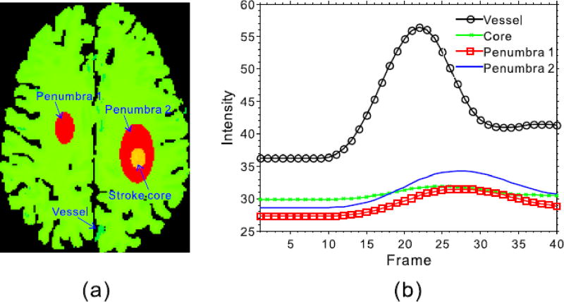
Fig. 2 shows the digital brain perfusion phantom used in this study which consists of user-defined regions of white matter, gray matter, penumbra, and stroke core [12]. We simulated the same phantom with the size of 256×256×40 as the previous work [11], which was designed to simulate a complex structure in real human brain. Specifically, a fan-beam CT imaging geometry was used in the simulation study, and the imaging parameters are set as follows: (1) each scan includes 1160 projection views evenly distributed over 2 π, (2) the number of channels per view is 672, and (3) the source-to-axis distance is 570 mm and the source-to-imager is 1040 mm. After the noise-free sinogram data ŷ, then noisy measurements z can be generated as follows:

$$z~\mathit{\text{Poisson}}(z_0\text{ exp}(-\hat{y}))+\mathit{\text{Gaussian}}(0,{\sigma }_e^2),$$ (31)

where z₀ denotes the incident flux and set to be 6.88×10⁴, 1.23×10⁵, and 1.58×10⁵ for 20 mAs, 40 mAs, and 50 mAs, respectively. ${\sigma }_e^2$ denotes the electronic background noise variance and is set to be 11. Three noise levels related to the projection data acquired about 20, 40 and 50 mAs at a fixed kVp were simulated.

Fig. 2.

Illustration for the digital brain perfusion phantom (a), and corresponding TDCs (b).

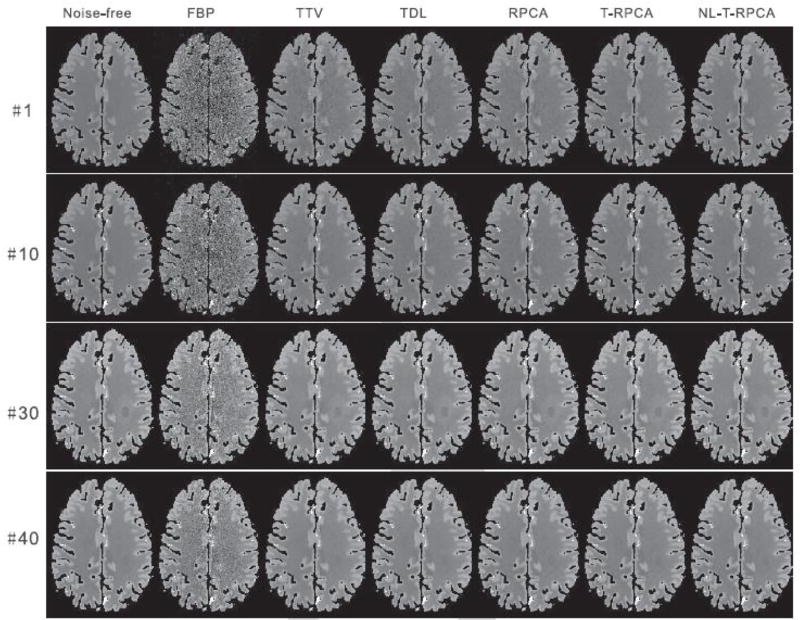
Fig. 3 shows the reconstructed four representative DCPCT frames of the digital brain phantom at 40 mAs. The first column shows the noise-free images that are used as the reference. As visualized in the results, the FBP reconstructed images are corrupted by severe noise-induced artifacts, and the TTV reconstructed images have a non-uniform intensity distribution in the homogeneous area and some details are smoothed out. Although the TDL algorithm can suppress noise-induced artifacts to some degree, some details were still lost. Furthermore, the RPCA-based algorithms can provide significantly improved image quality from the FBP and TTV algorithms. Note that the infarct core and penumbra tissue regions can be clearly observed in the T-RPCA and NL-T-RPCA images, suggesting that the spatial resolution is well preserved.

Fig. 3.

The noise-free images and low-dose CT images reconstructed by the different algorithms at time frames #1, #10, #30, and #40 at 40 mAs. All the images are displayed with the same window: [10 60] HU.

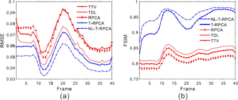
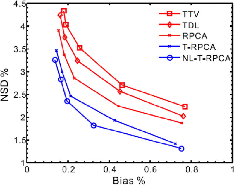
To better demonstrate the advantage of the proposed T-RPCA and NL-T-RPCA algorithms over the other algorithms, Fig. 4 illustrates the quantitative assessment of the low-dose DCPCT reconstructed images in terms of global root mean squared error (RMSE) and global feature similarity (FSIM) index [31] measurements. From Fig. 4 (a), it can be seen that the proposed T-RPCA algorithms exhibit an average of more than 29.8%, 7.84% and 28.6% gains over the TTV, TDL and RPCA algorithms, and the proposed NL-T-RPCA algorithms exhibit an average of more than 51.5%, 25.8% and 50.0% gains over the TTV, TDL and RPCA algorithms, respectively. In Fig. 4 (b), the T-RPCA and NL-T-RPCA algorithms obtain remarkably larger FSIM measurements than other three competing algorithms in all frames, confirming the visual observations. To further compare the performance of the various algorithms, Fig. 5 shows the local normalized standard deviation (NSD) versus Bias tradeoff curves of low dose reconstructed DCPCT images for all the SIR algorithms wherein a homogeneous region of interest (ROI) with the penumbra 1 is selected. It can be seen that the proposed NL-T-RPCA algorithm followed by the proposed T-RPCA algorithm has the best NSD-versus-Bias trade-off.

Fig. 4.

The global RMSE (a) and FSIM(b) measurements of the DCPCT images reconstructed by the different algorithms at 40 mAs.

Fig. 5.

The NSD versus Bias tradeoff curves of low-dose reconstructed DCPCT images for all the SIR algorithms at 40 mAs.

To further validate the proposed T-RPCA and NL-T-RPCA algorithms for hemodynamic parameter maps estimation, the reconstructed DCPCT images are utilized to estimate the CBF maps using the image-based deconvolution algorithm [18], i.e., bSVD. Fig. 6 illustrates representative CBF maps calculated from the ground truth and low-dose DCPCT images reconstructed by the different algorithms, the universal quality index (UQI) measurements being given in Table I. All the SIR algorithms can suppress the serious noise-induced artifacts effectively and show more accurate CBF estimates than the FBP algorithm. Moreover, the proposed T-RPCA and NL-T-RPCA algorithms are able to estimate the actual CBF maps with greater accuracy than the other algorithms. More details are listed in our supplementary material.

Fig. 6.

The CBF maps calculated by the bSVD algorithm from the different algorithms at 40 mAs. The unit is ml/100g/min.

TABLE I.

The UQI Values From the Different CBF Maps Estimated by the Different Algorithms at 40 mAs

Methods	FBP	TTV	TDL	RPCA	T-RPCA	NL-T-RPCA
UQI	0.7832	0.9855	0.9871	0.9898	0.9914	0.9925

B. Preclinical Study

In this study, the preclinical monkey study was approved by the institutional clinical trials review and the institutional animal care and use committee. In the preclinical experiment, two male monkeys with the middle cerebral artery occlusion were carried on a DCPCT examination with a GE Lightspeed pro 16 CT scanner. The monkeys were scanned before 20 mL iohexol (370 mgI/mL) was injected at 2 mL/second and then 98 second acquisition at 1 rotation per second, with FOV of 18 cm×18 cm, tube voltage of 80 kVp, and tube current of 200 mA. These acquired DCPCT data at high-dose were considered the reference standard for comparison to lower-dose DCPCT. To reduce radiation dose, instead of scanning the monkeys twice, we simulated the low-dose DCPCT data from these acquired DCPCT data. For low-dose DCPCT data, we simulate them from the reference standard using the simulation technique based on [11] which is similar to the simulation in Sec. III-A, and the noise levels related to the projection data acquired about 50 mA at a fixed kV p were simulated.

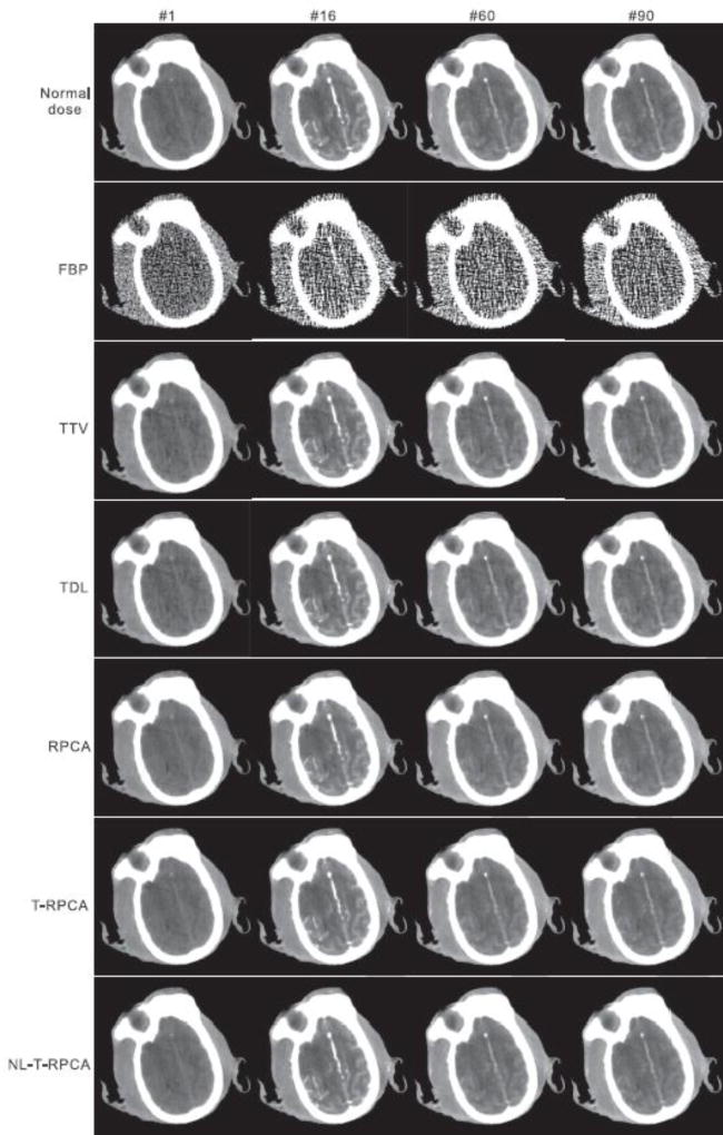
Fig. 7 illustrates the results from the preclinical monkey 1 data for different algorithms. The first row is the normal-dose DCPCT images used as the ground truth for evaluation. It was found that all the SIR reconstructed DCPCT images exhibit less noise-induced artifacts than the FBP results.

Fig. 7.

The normal-dose DCPCT images and low-dose DCPCT images reconstructed by the different algorithms at time frames #1, #20, #60, and #90 from the preclinical monkey 1 data. All the images are displayed with the same window: [800 1800]HU.

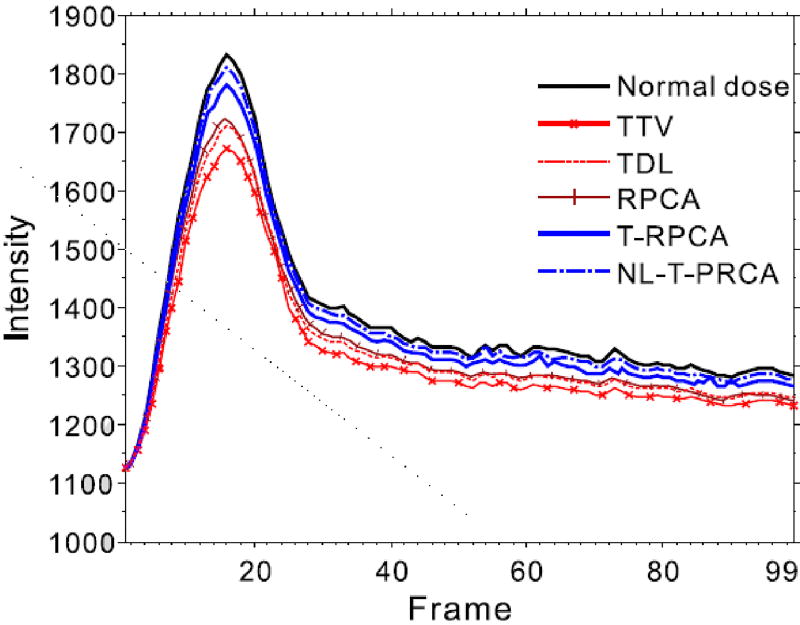
Fig. 8 shows the TDCs from the normal-dose DCPCT images and low-dose DCPCT images reconstructed by different algorithms. The selective ROI is indicated by red box in Fig. 7. It can be observed that the proposed T-RPCA and NL-T-RPCA algorithms show more accurate TDCs estimates than the other algorithms comparing with the ground truth.

Fig. 8.

The TDC’s curve calculated from normal-dose DCPCT images and low-dose DCPCT images reconstructed by the different algorithms from the preclinical monkey 1 data.

In addition, Fig. 9 shows representative CBF maps from the normal-dose and low-dose DCPCT images reconstructed by different competing algorithms. From the results, it can be observed that the SIR-based algorithms have led to significant improvements in the CBF map quality. In particular, the proposed T-RPCA and NL-T-RPCA algorithms exhibit smaller relative l₂-errors [32] in the estimated CBF in comparison to other algorithms, and the corresponding results are listed in Table II.

Fig. 9.

The CBF maps calculated from all competing algorithms from the preclinical monkey 1 data: (a) Normal dose; (b) FBP; (c) TTV; (d) TDL;(e) RPCA; (f) T-RPCA; and (g) NL-T-RPCA. The unit is ml/100g/min.

TABLE II.

The Relative l₂-Errors Measurements Over the CBF Maps Reconstructed by the Different Algorithms From the Preclinical Monkey 1 Data

Methods	TTV	TDL	RPCA	T-RPCA	NL-T-RPCA
Relative l2-errors	32.1%	28.6%	17.3%	12.2%	10.8%

In this study, the preclinical monkey data can be used to calculate the blood-brain barrier permeability (BBBP) map that is a valuable indicator to predict hemorrhagic transformation in the acute stroke region. Fig. 10 shows the BBBP maps calculated from the normal-dose and low-dose DCPCT images reconstructed by the different algorithms. It can be seen that the clearly delineated signal with clear-cut edges in the two proposed tensor-based RPCA images are better that those from the other algorithms.

Fig. 10.

The BBBP maps calculated from all competing algorithms from the preclinical monkey 1 data: (a) Normal dose; (b) FBP; (c) TTV; (d) TDL;(e) RPCA; (f) T-RPCA; and (g) NL-T-RPCA. The unit is HU.

C. Clinical Patient Study

Under written consent, the projection data of five patients with brain deficits were acquired using a GE Discovery CT750 HD scanner with helical scanning mode, and these clinical data serve as a pilot clinical study. The patients were scanned before approximately 45 mL nonionic iodinated contrast was administered intravenously at 4 mL/second. The CTP protocol consisted of 27 volumetric acquisitions which started with a high dose acquisition at 200 mA, 5 s after contrast injection, followed by 26 scans every 0.4 s at 70 mA. The X-ray tube voltage was 80 kV p, and the tube current was about 28 mAs which was considered as low-dose scan in clinic.

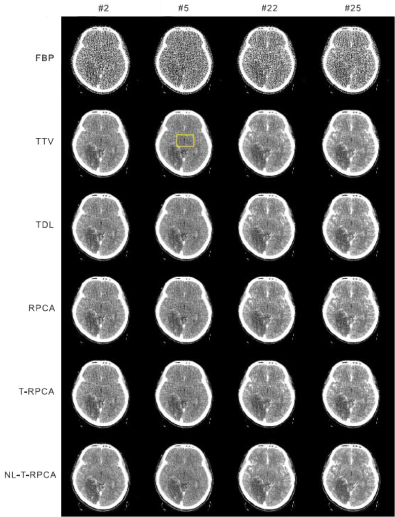
Fig. 11 shows the reconstructed DCPCT images in four representative frames from the clinical patient 1 data for the different algorithms. From the results, it can be observed that the image noise is effectively suppressed by the SIR-based algorithms. It is worth mentioning that the proposed T-RPCA and NL-T-RPCA algorithms can achieve great noise suppression at the same time preserve detail information. More details are listed in our supplementary material.

Fig. 11.

The clinical patient 1 data reconstructed by the FBP, TTV, TDL RPCA, T-RPCA and proposed NL-T-algorithms at time frames #1, #10, #15 and #26. All the images are displayed with the same window: [1000 1300] HU.

To further qualitatively illustrate the clinic application of the CBF maps calculated from the reconstructed DCPCT images for the competing algorithms as shown in Fig. 12, 5 experienced physicians are asked to score the low-dose CBF maps from 0 (worst) to 5 (best) in terms of the following attributes: image noise, artifacts, edge and structure, and stroke region estimation. In this work, the low-dose CBF maps estimated by all utilized comparison algorithms are displayed on the screen randomly, therefore, the test was a completely blind process for all the physicians. The corresponding physicians scores are listed in Table III. It is evident that the CBF maps calculated by the proposed T-RPCA and NL-T-RPCA algorithms compare favorably to the other algorithms in terms of visual inspection and subjective assessment scores. More details are listed in our supplementary material.

Fig. 12.

The CBF maps calculated from the low-dose DCPCT images from the clinical patient 1 data reconstructed by the different algorithms: (a) TTV; (b) TDL; (c) RPCA; (d) T-RPCA; and (e) NL-T-RPCA. The unit is ml/100g/min.

TABLE III.

The Physician’s Scores of the Estimated CBF Maps From the Different Algorithms in the 5 Clinical Patients Studies

Methods	TTV	TDL	RPCA	T-RPCA	NL-T-RPCA
Score	3.35±0.81	3.42±0.61	3.71±0.58	4.38±0.37	4.51±0.32

IV. DISCUSSIONS AND CONCLUSIONS

In clinic, the DCPCT images can be inherently represented as a superposition of “background” component, which is almost static over time, and a dynamic component, which is rapidly changing over time. The “background” component corresponds to high spatial-temporal correlations among frames which can be assumed to be low-rank (L), and the dynamic component is time-varying and spatial-temporal consecutive which can be assumed to be sparse (S) or transform-sparse [20], [21]. The L+S decomposition can be utilized to perform RPCA to recover the principal components of a data matrix with missing or corrupted entries [20]. Up to now, RPCA (or, equivalently the L+S decomposition) has been successfully applied to computer vision, such as video sequence [33], image alignment [34], and medical imaging [20]. To better take the spatial and temporal structure of “background” component into consideration more comprehensively, in this work, we extend matrix-based “background” component representation to the tensor-based “background” component representation, and then present two tensor-based RPCA models, i.e., T-RPCA and NL-T-RPCA, for low-dose DCPCT images reconstruction. The two proposed models are performed on the entire spatial-temporal DCPCT data, instead of each frame individually. In particular, the NL-T-RPCA model further considers the intrinsic characteristics underlying the DCPCT images, i.e., nonlocal self-similarity and global correlation, describing the 3D block groups of the “background” part in a tensor. To the best of our knowledge, this is the first study to investigate the impact of tensor-based RPCA model as applied to the DCPCT images for quantification of the TDC curves and CBF maps. The experiments are conducted with a digital brain phantom, preclinical monkey data and clinical patient data from low-dose acquisitions. Results of visualization and quantitative studies in Section III demonstrated that the two proposed tensor-based RPCA models work remarkably better than the other algorithms in terms of several quality-measure-utility metrics used in low-dose cases, especially as low as 20 mAs.

In the two proposed tensor-based models, some parameters, i.e., hyper-parameters ζ and γ in the T-RPCA model, and the size of tensor patch s_m, s_n and s_t, and the size of search window, the number of the similar patches P, rank parameters s₁, s₂, s₃ and s₄, and hyper-parameter γ in the NL-T-RPCA model, should be optimally selected to yield acceptable results. It should be noted that determining the optimal them for the proposed models is still an open question. In this study, we have adopted an empirical method to select the hyper parameters and rank parameters, choosing those presenting the best reconstruction performance over a broader range of possible values. Although this process might be time-consuming, the parameters might be varied by the given dataset, and special care is necessary to select the right ones to obtain acceptable results, it needs to be undertaken only once for each target object, i.e., digital phantom, preclinical data, or patient data; and the same parameters can be used for subsequent studies with similar dynamic information. Of particular note is some strategies on automatic parameters selection of matrix completion might be applied to the proposed tensor-based models. In addition, the size of tensor patch s_m, s_n and s_t, and the size of search window, the number of the similar patches P are determined by trying several combinations of parameters. Shared with other SIR algorithms, combing with tensor-based operation, the two proposed tensor-based models are iterative and computational expensive, especially for the NL-T-RPCA model that includes the search of 3D similar patches and joint Tucker decomposition. The computational cost of the T-RPCA and NL-T-RPCA algorithms were approximately 18.2 and 27.3 minutes in processing the digital brain perfusion phantom with the size of 256 × 256 × 40 at each iteration step. Fast computer with GPU-assisted implementation is expected to dramatically accelerate the associated computation for possible clinical practice.

The work suggests other interesting points meriting future study. In our study, all the cases are assumed no motion, indicting two consecutive scans should not differ significantly (i.e., only form noise), and therefore motion is of minimal concern. However, some involuntary motion may be sometimes unavoidable during vivo scanning. To address this issue, techniques should be developed to incorporate motion compensation along with the SIR framework to improve image quality further. In addition, the data were acquired from limited sample of patients and potential selection bias is unknown. Review of a clinical study with a variety of patients would be beneficial to demonstrate whether the proposed tensorbased models can be extended to a broader population. In the future, to improve the performance, the image-domain iterative deconvolution algorithm [9]–[11] can be introduced into the proposed tensor-based model framework to obtain better CBF maps.

References

- 1.Hoeffner EG, et al. Cerebral perfusion CT: Technique and clinical applications. Radiology. 2004 Aug.231:632–644. doi: 10.1148/radiol.2313021488. [DOI] [PubMed] [Google Scholar]
- 2.Othman AE, et al. Radiation dose reduction in perfusion CT imaging of the brain: A review of the literature. J. Neuroradiol. 2015 Oct.43:1–5. doi: 10.1016/j.neurad.2015.06.003. [DOI] [PubMed] [Google Scholar]
- 3.Saito N, et al. Realization of reliable cerebral-blood-flow maps from low-dose CT perfusion images by statistical noise reduction using nonlinear diffusion filtering. Radiol. Phys. Technol. 2008 Jan.1:62–74. doi: 10.1007/s12194-007-0009-7. [DOI] [PubMed] [Google Scholar]
- 4.Mendrik AM, et al. TIPS bilateral noise reduction in 4D CT perfusion scans produces high-quality cerebral blood flow maps. Phys. Med. Biol. 2011;56(13):3857–3872. doi: 10.1088/0031-9155/56/13/008. [DOI] [PubMed] [Google Scholar]
- 5.Ma J, et al. Low-dose computed tomography image restoration using previous normal-dose scan. Med. Phys. 2011;38(10):5713–5731. doi: 10.1118/1.3638125. [DOI] [PMC free article] [PubMed] [Google Scholar]
- 6.Supanich M, et al. Radiation dose reduction in time-resolved CT angiography using highly constrained back projection reconstruction. Phys. Med. Biol. 2009;54(14):4575–4593. doi: 10.1088/0031-9155/54/14/013. [DOI] [PMC free article] [PubMed] [Google Scholar]
- 7.He L, et al. A spatio-temporal deconvolution method to improve perfusion CT quantification. IEEE Trans. Med. Imag. 2010 May;29(5):1182–1191. doi: 10.1109/TMI.2010.2043536. [DOI] [PubMed] [Google Scholar]
- 8.Boutelier T, Kudo K, Pautot F, Sasaki M. Bayesian hemodynamic parameter estimation by bolus tracking perfusion weighted imaging. IEEE Trans. Med. Imag. 2012 Jul.31(7):1381–1395. doi: 10.1109/TMI.2012.2189890. [DOI] [PubMed] [Google Scholar]
- 9.Fang R, Chen T, Sanelli PC. Towards robust deconvolution of low-dose perfusion CT: Sparse perfusion deconvolution using online dictionary learning. Med. Image Anal. 2013;17(4):417–428. doi: 10.1016/j.media.2013.02.005. [DOI] [PMC free article] [PubMed] [Google Scholar]
- 10.Fang R, Zhang S, Chen T, Sanelli PC. Robust low-dose CT perfusion deconvolution via tensor total-variation regularization. IEEE Trans. Med. Imag. 2015 Jul.34(7):1533–1548. doi: 10.1109/TMI.2015.2405015. [DOI] [PMC free article] [PubMed] [Google Scholar]
- 11.Zeng D, et al. Cerebral perfusion computed tomography deconvolution via structure tensor total variation regularization. Med. Phys. 2016;43(5):2091–2107. doi: 10.1118/1.4944866. [DOI] [PubMed] [Google Scholar]
- 12.Manhart MT, et al. Dynamic iterative reconstruction for interventional 4-D C-arm CT perfusion imaging. IEEE Trans. Med. Imag. 2013 Jul.32(7):1336–1348. doi: 10.1109/TMI.2013.2257178. [DOI] [PubMed] [Google Scholar]
- 13.Van Nieuwenhove V, et al. Local attenuation curve optimization framework for high quality perfusion maps in low-dose cerebral perfusion CT. Med. Phys. 2016;43(12):6429–6438. doi: 10.1118/1.4967263. [DOI] [PubMed] [Google Scholar]
- 14.Ma J, et al. Iterative image reconstruction for cerebral perfusion CT using pre-contrast scan induced edge-preserving prior. Phys. Med. Biol. 2012;57(22):7519–7542. doi: 10.1088/0031-9155/57/22/7519. [DOI] [PMC free article] [PubMed] [Google Scholar]
- 15.Li B, Lyu Q, Ma J, Wang J. Iterative reconstruction for CT perfusion with a prior-image induced hybrid nonlocal means regularization: Phantom studies. Med. Phys. 2016;43(4):1688–1699. doi: 10.1118/1.4943380. [DOI] [PMC free article] [PubMed] [Google Scholar]
- 16.Tian X, et al. Robust low-dose dynamic cerebral perfusion CT image restoration via coupled dictionary learning scheme. J X-Ray Sci. Technol. 2016;24(6):837–853. doi: 10.3233/XST-160593. [DOI] [PubMed] [Google Scholar]
- 17.Niu S, et al. Low-dose cerebral perfusion computed tomography image restoration via low-rank and total variation regularizations. Neurocomputing. 2016 Jul.197:143–160. doi: 10.1016/j.neucom.2016.01.090. [DOI] [PMC free article] [PubMed] [Google Scholar]
- 18.Wu O, Østergaard L, Weisskoff RM, Benner T, Rosen BR, Sorensen AG. Tracer arrival timing-insensitive technique for estimating flow in MR perfusion-weighted imaging using singular value decomposition with a block-circulant deconvolution matrix. Magn. Reson. Med. 2003;50(1):164–174. doi: 10.1002/mrm.10522. [DOI] [PubMed] [Google Scholar]
- 19.Inal T, Telatar Z, Atac GK. Noise reduction in CT perfusion images: A bilateral filter trial. Proc. IEEE Signal Process. Commun. Appl. Conf. 2014 Apr.670:184–187. [Google Scholar]
- 20.Gao H, Cai JF, Shen Z, Zhao H. Robust principal component analysis-based four-dimensional computed tomography. Phys. Med. Biol. 2011;56(11):3181–3198. doi: 10.1088/0031-9155/56/11/002. [DOI] [PMC free article] [PubMed] [Google Scholar]
- 21.Cao W, et al. Total variation regularized tensor RPCA for background subtraction from compressive measurements. IEEE Trans. Image Process. 2016 Sep.25(9):4075–4090. doi: 10.1109/TIP.2016.2579262. [DOI] [PubMed] [Google Scholar]
- 22.Tucker LR. Some mathematical notes on three-mode factor analysis. Psychometrika. 1966;31(3):279–311. doi: 10.1007/BF02289464. [DOI] [PubMed] [Google Scholar]
- 23.Kolda TG, Bader BW. Tensor decompositions and applications. SIAM Rev. 2009;51(3):455–500. [Google Scholar]
- 24.Ma J, et al. Variance analysis of x-ray CT sinograms in the presence of electronic noise background. Med. Phys. 2012;39(7):4051–4065. doi: 10.1118/1.4722751. [DOI] [PMC free article] [PubMed] [Google Scholar]
- 25.Xie Q, et al. Proc. IEEE Conf. Comput. Vis. Pattern Recognit. (CVPR) Las Vegas, NV, USA: Jun. 2016. Multispectral images denoising by intrinsic tensor sparsity regularization; pp. 1692–1700. [Google Scholar]
- 26.Karimi D, Ward RK. Patch-based models and algorithms for image processing: A review of the basic principles and methods, and their application in computed tomography. Int. J. Comput. Assist. Radiol. Surg. 2016;11(10):1–13. doi: 10.1007/s11548-016-1434-z. [DOI] [PubMed] [Google Scholar]
- 27.Boyd S, Parikh N, Chu E, Peleato B, Eckstein J. Distributed optimization and statistical learning via the alternating direction method of multipliers. Found. Trends Mach. Learn. 2011 Jan.3(1):1–122. [Google Scholar]
- 28.Candès EJ, Wakin MB, Boyd SP. Enhancing sparsity by reweighted 1 minimization. J Fourier Anal. Appl. 2008;14(5–6):877–905. [Google Scholar]
- 29.Gong P, Zhang C, Lu Z, Huang JZ, Ye J. A general iterative shrinkage and thresholding algorithm for non-convex regularized optimization problems. Proc. Int. Conf. Mach. Learn. 2013;28:37–45. [PMC free article] [PubMed] [Google Scholar]
- 30.Zhang Y, Mou X, Wang G, Yu H. Tensor-based dictionary learning for spectral CT reconstruction. IEEE Trans. Med. Imag. 2016 Jan.36(1):142–154. doi: 10.1109/TMI.2016.2600249. [DOI] [PMC free article] [PubMed] [Google Scholar]
- 31.Zhang L, Zhang L, Mou X, Zhang D. FSIM: A feature similarity index for image quality assessment. IEEE Trans. Image Process. 2011 Aug.20(8):2378–2386. doi: 10.1109/TIP.2011.2109730. [DOI] [PubMed] [Google Scholar]
- 32.Ehrhardt MJ, et al. Joint reconstruction of PET-MRI by exploiting structural similarity. Inverse Problems. 2015;31(1):015001. [Google Scholar]
- 33.Candès EJ, Li X, Ma Y, Wright J. Robust principal component analysis? J. ACM. 2011 Sep.58:1–37. [Google Scholar]
- 34.Peng Y, Ganesh A, Wright J, Xu W, Ma Y. RASL: Robust alignment by sparse and low-rank decomposition for linearly correlated images. IEEE Trans. Pattern Anal. Mach. Intell. 2012 Nov.34(11):2233–2246. doi: 10.1109/TPAMI.2011.282. [DOI] [PubMed] [Google Scholar]
Associated Data
This section collects any data citations, data availability statements, or supplementary materials included in this article.