Feature selection and classifier performance in computer-aided diagnosis: The effect of finite sample size

Abstract

In computer-aided diagnosis (CAD), a frequently used approach for distinguishing normal and abnormal cases is first to extract potentially useful features for the classification task. Effective features are then selected from this entire pool of available features. Finally, a classifier is designed using the selected features. In this study, we investigated the effect of finite sample size on classification accuracy when classifier design involves stepwise feature selection in linear discriminant analysis, which is the most commonly used feature selection algorithm for linear classifiers. The feature selection and the classifier coefficient estimation steps were considered to be cascading stages in the classifier design process. We compared the performance of the classifier when feature selection was performed on the design samples alone and on the entire set of available samples, which consisted of design and test samples. The area A_z under the receiver operating characteristic curve was used as our performance measure. After linear classifier coefficient estimation using the design samples, we studied the hold-out and resubstitution performance estimates. The two classes were assumed to have multidimensional Gaussian distributions, with a large number of features available for feature selection. We investigated the dependence of feature selection performance on the covariance matrices and means for the two classes, and examined the effects of sample size, number of available features, and parameters of stepwise feature selection on classifier bias. Our results indicated that the resubstitution estimate was always optimistically biased, except in cases where the parameters of stepwise feature selection were chosen such that too few features were selected by the stepwise procedure. When feature selection was performed using only the design samples, the hold-out estimate was always pessimistically biased. When feature selection was performed using the entire finite sample space, the hold-out estimates could be pessimistically or optimistically biased, depending on the number of features available for selection, the number of available samples, and their statistical distribution. For our simulation conditions, these estimates were always pessimistically (conservatively) biased if the ratio of the total number of available samples per class to the number of available features was greater than five.

I. INTRODUCTION

Computer-aided interpretation of medical images has been the subject of numerous studies in recent years. The purpose of computer-aided diagnosis (CAD) in medical imaging is to provide a second opinion to the radiologist concerning the presence or the likelihood of malignancy of abnormalities in a given image or case. The general visual criteria that help describe the abnormality or its classification can usually be provided by the radiologist. However, in many cases, it is difficult to translate these criteria into computer algorithms that exactly match the verbal description of what the radiologist visually perceives. Therefore, a common first step in CAD is to extract a number of features, or a feature space, that is believed to have a potential for the given task. The features may or may not match to what a radiologist searches in the image for the same task. In the next step, a subset of features are selected from the entire feature space based on their individual or joint performance, and the selected set of features are used in the remaining steps of the CAD system. This approach also has the advantage that the computer may discover some features that are difficult to perceive or verbally describe by the radiologist, so that the computer may extract information that is complementary to the radiologist’s perceived image features.

A common problem in CAD is the lack of a large number of image samples to design a classifier and to test its performance. Although the effect of finite sample size on classification accuracy has previously been studied, many elements of this research topic warrant further study. In order to treat specific components of this problem, previous studies have mostly ignored the feature selection component of this problem, and assumed that the features to be used in the classifier have been chosen and are fixed.^1–6 However, as described in the previous paragraph, feature selection is a necessary first step in many CAD algorithms. This paper addresses the effect of finite sample size on classification accuracy when the classifier design involves feature selection.

When only a finite number of samples are available for classifier design and testing, two commonly used performance estimates are those provided by the resubstitution and the hold-out methods. In the hold-out method, the samples are partitioned into independent training and test samples, the classifier is designed using the training samples alone, and the accuracy of the designed classifier is measured by its performance for the test samples. In the resubstitution method, the accuracy is measured by applying the classifier to the training samples that have been used to design it. Other methods such as leave-one-out and bootstrap have also been shown to be very useful procedures for performance estimation with a finite sample size.⁷ As the number of training samples increases, all of these estimates approach the true classification accuracy, which is the accuracy of a classifier designed with the full knowledge of the population distributions. When the training sample size is finite, it is known that, on average, the resubstitution estimate of classifier accuracy is optimistically biased relative to that of a classifier trained with an infinite sample. In other words, it has a higher expected value than the performance obtained with an infinite design sample set, which is the true classification accuracy. Similarly, on average, the hold-out estimate is pessimistically biased, i.e., it has a lower expected value than the true classification accuracy. When classifier design is limited by the availability of design samples, it is important to obtain a realistic estimate of the classifier performance so that classification will not be misled by an optimistic estimate such as that provided by resubstitution.

In CAD literature, different methods have been used to estimate the classifier accuracy when the classifier design involves feature selection. In a few studies, only the resubstitution estimate was provided.⁸ In some studies, the researchers partitioned the samples into training and test groups at the beginning of the study, performed both feature selection and classifier parameter estimation using the training set, and provided the hold-out performance estimate.^9,10 Most studies used a mixture of the two methods. The entire set of available samples was used as the training set at the feature selection step of classifier design. Once the features have been chosen, the hold-out or leave-one-out methods were used to measure the accuracy of the classifier.^11–16 To our knowledge, it has not been reported whether this latter method provides an optimistic or pessimistic estimate of the classifier performance.

A powerful method for estimating the infinite-sample performance of a classifier using a finite number of available samples was first suggested by Fukunaga and Hayes.¹⁷ In the Fukunaga–Hayes method, subsets of N₁, N₂,…,N_j design samples are drawn from the available sample set, the classifier accuracy is evaluated at these different sample sizes, and the infinite-sample performance is estimated by linear extrapolation from the j points to N→∞ or 1/N→0. This method has recently been applied to performance estimation in CAD, where the area A_z under the receiver operating characteristic (ROC) curve is commonly used as the performance measure.^1–3 For various classifiers and Gaussian sample distributions, the A_z value was plotted against 1/N_i, and it was observed that the dependence of the A_z value can be closely approximated by a linear relationship in a sample size range where higher-order terms in 1/N_i can be neglected.^1–3 This facilitates estimation of the infinite-sample performance from the intercept of a linear regression.

This paper describes a simulation study that investigates the effect of finite sample size on classifier accuracy when classifier design involves feature selection using stepwise linear discriminant analysis. The classification problem was defined as deciding whether a sample belongs to either one of two classes, and the two classes were assumed to have multivariate Gaussian distributions with equal covariance matrices. We chose to focus our attention on stepwise feature selection in linear discriminant analysis since this is a commonly used feature selection and classification method. The effects of different covariance matrices and means on feature selection performance were studied. We examined the effects of sample size, number of available features, and parameters of stepwise feature selection on classifier bias. The biases of the classifier performance when feature selection was performed on the entire sample space and on the design samples alone were compared. Finally, we investigated whether the methods of infinite-sample performance estimation developed previously^1–3,17 can be applied to our problem.

II. METHODS

In our approach, the problem of classifier design is analyzed in two stages. The first stage is stepwise feature selection, and the second stage is the estimation of the coefficients in the linear discriminant formulation using the selected feature subset as predictor variables.

A. Stepwise feature selection

The two-class classification defined in the last paragraph of the Introduction can be formulated as a first-order linear multiple regression problem.¹⁸ Since most of the literature on stepwise feature selection is based on the linear regression formulation, we will use this formulation to describe stepwise feature selection in this subsection. A different statistical formulation of the problem, which coincides with the linear regression formulation if the covariance matrices of the classes are equal,¹⁸ will be described in Sec. II A, and will be used in the remainder of the paper.

Let N denote the number of samples available to design the classifier, and let k denote the number of features. In the linear multiple regression formulation, a desired output o(i) is assigned to each k-dimensional feature vector X_i such that

$$o(i)=\{\begin{array}{cc}{o}_1\hfill & \text{if }i\in \text{class }1\hfill \\ o_2\hfill & \text{if }i\in \text{class }2\hfill \end{array}.$$ (1)

To define the linear multiple regression problem, the desired outputs o(i) are used as the dependent variable and the feature vectors X_i are used as the independent variables. The discriminant score for a feature vector X_i is the predicted value of o(i), computed by the regression equation

$$h^{(k)}(X_i)=b^T{X}_i+b_0,$$ (2)

where b^T=[b₁, b₂,…,b_k] and b₀ are the regression coefficients. Stepwise feature selection iteratively changes the number of features k used in the classification by entering features into or removing features from the group of selected features based on a feature selection criterion using F-statistics.^19,20 We have used stepwise feature selection for classifier design in many of our CAD applications.^11,21–23 In this study, Wilks’ lambda, which is defined as the ratio of within-group sum of squares to the total sum of squares of the discriminant scores, was used as the feature selection criterion. Let $m_1^{(k)}$ and $m_2^{(k)}$ denote the means of the discriminant scores for classes 1 and 2, respectively, and let m^(k) denote the mean of the discriminant scores computed over both classes. Wilks’ lambda λ_k is defined as¹⁹

$${\lambda }_k=\frac{{\sum }_{i\in \text{class }1}{(h^{(k)}(X_i)-m_1^{(k)})}^2+{\sum }_{i\in \text{class }2}{(h^{(k)}(X_i)-m_2^{(k)})}^2}{{\sum }_{i=1}^N{(h^{(k)}(X_i)-m^{(k)})}^2}.$$ (3)

A smaller value for Wilks’ lambda means that the spread within each class is small compared with the spread of the entire sample, which means the separation of the two classes is relatively large and that better classification is possible. Entering a new feature into regression will always decrease Wilks’ lambda, unless the feature is completely useless for classifying the available samples. The problem is to decide whether the decrease in Wilks’ lambda justifies entering the feature into regression. In stepwise feature selection an F-to-enter value—for making the decision whether a feature should be entered when k features are already used—is defined as²⁴

$$F=(N-k-2)(\frac{{\lambda }_k}{{\lambda }_{k+1}}-1),$$ (4)

where λ_k is Wilks’ lambda before entering the feature, and λ_k+1 is Wilks’ lambda after entering the feature. An F-to-remove value is similarly defined to decide whether a feature already in the regression should be removed. At the feature entry step of the stepwise algorithm, the feature with the largest F-to-enter value is entered into the selected feature pool if this maximum value is larger than a threshold F_in. At the feature removal step, the feature with the smallest F-to-remove value is removed from the selected feature pool if this minimum value is smaller than a threshold F_out. The algorithm terminates when no more features can satisfy the criteria for either entry or removal. The number of selected features increases, in general, when F_in and F_out are reduced.

In order to avoid numerical instabilities in the solution of linear systems of equations, a tolerance term is also employed in the stepwise procedure to exclude highly correlated features. If the correlation between a new feature and the already selected features is larger than a tolerance threshold, then the feature will not be entered into the selected feature pool even if it satisfies the feature entry criterion described in the previous paragraph.

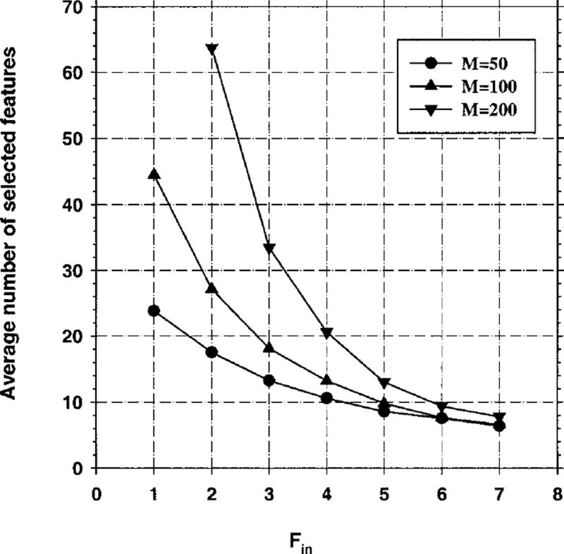
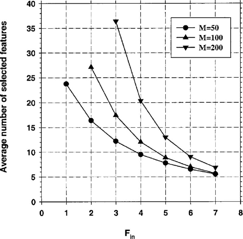
Since the optimal values of F_in and F_out for a given classification task are not known a priori, these thresholds have to be varied over a range in order to find the “best” combinations of features in a practical application. In this simulation study, we limit our selection of F_out to F_out=F_in − 1, so that we do not search through all combinations of F values. This constraint should not limit our ability to demonstrate the effect of finite sample size on feature selection and classifier performance, because we were still able to vary the number of selected features over a wide range, as will be shown in Figs. 6 and 12 below.

Fig. 6.

Case 1 (identity covariance matrix), A_z(∞) = 0.89. Feature selection from the entire sample space of 100 samples/class: The number of features selected in stepwise feature selection versus F_in(F_out = F_in − 1).

Fig. 12.

Case 1 (identity covariance matrix), A_z(∞) = 0.89. Feature selection from N_t = 80 design samples per class. Total sample size N_s = 100 samples per class. The number of features selected in stepwise feature selection versus F_in(F_out = F_in − 1).

B. Estimation of linear discriminant coefficients

As a by-product of the stepwise feature selection procedure used in our study, the coefficients of a linear discriminant classifier that classifies the design samples using the selected features as predictor variables are also computed. However, in this study, the design samples of the stepwise feature selection may be different from those used for coefficient estimation in the linear classifier. Therefore, we implemented the stepwise feature selection and discriminant coefficient estimation components of our classification scheme separately.

Let Σ₁ and Σ₂ denote the k-by-k covariance matrices of samples belonging to class 1 and class 2, and let μ₁=(μ₁(1), μ₁(2),…,μ₁(k)), μ₂=(μ₂(1), μ₂(2),…,μ₂(k)) denote their mean vectors. For an input vector X, the linear discriminant classifier output is defined as

$$h(X)={({\mu }_2-{\mu }_1)}^T{\sum }^{-1}X+\frac{1}{2}({\mu }_1^T{\sum }^{-1}{\mu }_1-{\mu }_2^T{\sum }^{-1}{\mu }_2),$$ (5)

where Σ = (Σ₁ + Σ₂)/2. Because of the assumption in this study that the two covariance matrices are equal, Σ reduces to Σ = Σ₁ = Σ₂. Therefore, we will be concerned with only the form of Σ in the following discussions. The linear discriminant classifier is the optimal classifier when the two classes have a multivariate Gaussian distribution with equal covariance matrices.

For the class separation measures considered in this paper (refer to Sec. II C), the constant term $({\mu }_1^T{\sum }^{-1}{\mu }_1-{\mu }_2^T{\sum }^{-1}{\mu }_2)/2$ in Eq. (1) is irrelevant. Therefore, the classifier design can be viewed as the estimation of k parameters of the vector b = (μ₂ − μ₁)^TΣ⁻¹ using the design samples.

When a finite number of design samples are available, the means and covariances are estimated as the sample means and the sample covariances from the design samples. The substitution of the true means and covariances in Eq. (1) by their estimates causes a bias in the performance measure of the classifier. In particular, if the designed classifier is used for the classification of design samples, then the performance is optimistically biased. On the other hand, if the classifier is used for classifying test samples that are independent from the design samples, then the performance is pessimistically biased.

C. Measures of class separation

The traditional assessment methodology in medical imaging is receiver operating characteristic (ROC) analysis, which was first developed in the context of signal detection theory.^25–27 In this study, the output score of the classifier was used as the decision variable in ROC analysis, and the area A_z under the ROC curve was used as the principal measure of class separation. Excellent reviews of ROC methods applied to medical imaging can be found in the literature.^28–30

1. Infinite sample size

When an infinite sample size is available, the class means and covariance matrices can be estimated without bias. In this case, we use the squared Mahalanobis distance Δ(∞), or the area A_z(∞) under the ROC curve as the measures of class separation, as explained below. The infinity sign in parentheses denotes that the distance is computed using the true means and covariance matrices, or, equivalently, using an infinite number of random samples from the population.

Assume that two classes with multivariate Gaussian distributions and equal covariance matrices have been classified using Eq. (1). Since Eq. (1) is a linear function of the feature vector X, the distribution of the classifier outputs for class 1 and class 2 will be Gaussian. Let m₁ and m₂ denote the means of the classifier output for the case of the normal class, and for the case of the abnormal class, respectively, and let $s_1^2$ and $s_2^2$ denote the variances. With the squared Mahalanobis distance Δ(∞) defined as

$$\mathrm{\Delta }(\infty )={({\mu }_2-{\mu }_1)}^T{\sum }^{-1}({\mu }_2-{\mu }_1),$$ (6)

it can be shown that

$$m_2-m_1=s_1^2=s_2^2=\mathrm{\Delta }(\infty ).$$ (7)

The quantity Δ(∞) is referred to as the squared Mahalanobis distance between the two classes. It is the square of the Euclidean distance between the two classes, normalized to the common covariance matrix.

In particular, if Σ is a k-by-k diagonal matrix with Σ_i,i = σ²(i), then

$$\mathrm{\Delta }(\infty )=\sum _{i=1}^k\delta (i),$$ (8)

where

$$\delta (i)={[{\mu }_2(i)-{\mu }_1(i)]}^2/{\sigma }^2(i)$$ (9)

is the squared signal-to-noise ratio of the distributions of the two classes for the ith feature.

Using Eq. (3), and the normality of the classifier outputs, it can be shown that³¹

$$A_Z(\infty )=\frac{1}{\sqrt{2\pi }}{\int }_{-\infty }^{\sqrt{\mathrm{\Delta }/2}}{e}^{-t^2/2}\mathit{\text{dt}}.$$ (10)

2. Finite sample size

When a finite sample size is available, the means and covariances of the two class distributions are estimated as the sample means and the sample covariances using the design samples. The output score of the linear discriminant classifier for a test sample is computed using Eq. (1). The accuracy of the classifier in discriminating the samples from the two classes is measured by ROC methodology. The discriminant score is used as the decision variable in the labroc program,³² which provides the ROC curve based on maximum likelihood estimation.³³

D. Simulation conditions

In our simulation study, we assumed that the two classes follow multivariate Gaussian distributions with equal covariance matrices and different means. This assumption is an idealization of the real class distributions that one may observe in a practical classification problem. It restricts the number of parameters in our simulations to a manageable range, while permitting us to approximate a range of situations that may be encountered in CAD.

We generated a set of N_s samples from each class distribution using a random number generator. The sample space was randomly partitioned into N_t training samples and N_s−N_t test samples per class. For a given sample space, we used several different values for N_t in order to study the effect of the design sample size on classification accuracy. For a given N_t, the sample space was independently partitioned 20 times into N_t training samples and N_s − N_t test samples per class, and the classification accuracy A_z obtained from these 20 partitions was averaged in order to reduce the variance of the classification accuracy estimate. The procedure described above was referred to as one experiment. For each class distribution described in Cases 1, 2, and 3 below, 50 statistically independent experiments were performed, and the results were averaged.

Two methods for feature selection were considered. In the first method, the entire sample space with N_s samples per class was used for feature selection. In other words, the entire sample space was treated as a training set at the feature selection step of classifier design. After feature selection, the training-test partitioning was used to evaluate the resubstitution and hold-out performances of the coefficient estimation step of classifier design. In the second method, both feature selection and coefficient estimation were performed using only the training set with N_t samples per class.

Case 1: Identity covariance matrix

In the first simulation condition, a hypothetical feature space was constructed such that the covariance matrices of the two classes Σ₁ = Σ₂ = Σ was the identity matrix, and the mean difference Δμ between the two classes for feature i was

$$\mathrm{\Delta }\mu (i)={\mu }_2(i)-{\mu }_1(i)={\alpha \beta }^i,i=1,\dots ,M\text{ and }\beta <1,$$ (11)

where M refers to the number of available features for feature selection. Note that k, previously defined in Sec. II B, refers to the number of features selected for classifier parameter estimation; therefore, in general, M≥k. For a given data set, the number of available features M is fixed, whereas the number of selected features k depends on the F_in and F_out parameters of the stepwise selection algorithm. Since β is chosen to be less than 1, the ability for separation of the two classes by feature no. i decreased as i increased, as evidenced by δ (i) = (αβⁱ)² [see Eq. (5)]. The squared Mahalanobis distance Δ(∞) was computed as

$$\mathrm{\Delta }(\infty )=\frac{{\alpha }^2{\beta }^2}{1-{\beta }^2}(1-{\beta }^{2M})$$

since σ(i) = 1 for all i’s.

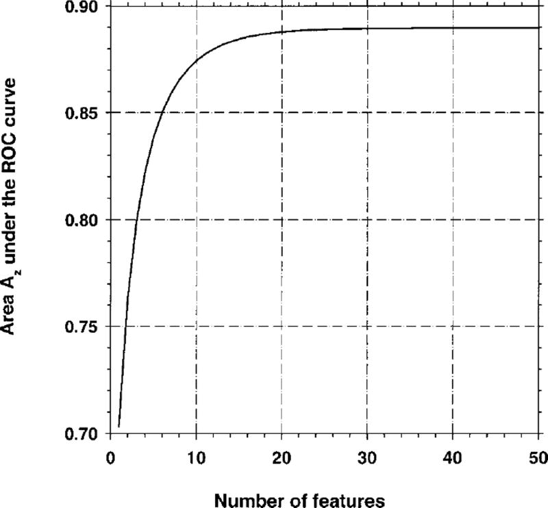
In our simulation, we chose β = 0.9, and chose α such that Δ(∞) = 3.0, or A_z(∞) = 0.89. The value of A_z(∞) versus k is plotted in Fig. 1, when features 1 through k were included in the linear discriminant. It is seen that for k>25, the contribution of an additional feature to the classification accuracy was very close to zero. With this simulation condition, we studied the classification accuracy for three different numbers of available features, namely, M = 50, M = 100, and M = 200.

Fig. 1.

The area A_z under the ROC curve versus the number of features, k, used in linear discriminant analysis for Case 1 (identity covariance matrix). In this figure, it is assumed that an infinite number of features are available for classifier training, and that features i = 1,2,…,k are used for classification.

Case 2: Comparison of correlated and diagonal covariance matrices

Case 2(a)

In this simulation condition, the number of available features was fixed at M = 100. In contrast to the simulation condition shown in Case 1 in this section, some of the features were assumed to have non-zero correlation. The covariance matrix Σ for the 100 features was assumed to have a block-diagonal structure

$$\sum =\left[\begin{array}{ccccc}A\hfill & 0\hfill & 0\hfill & \cdots \hfill & 0\hfill \\ 0\hfill & A\hfill & 0\hfill & \cdots \hfill & 0\hfill \\ 0\hfill & 0\hfill & A\hfill & \ddots \hfill & ⋮\hfill \\ ⋮\hfill & ⋮\hfill & \ddots \hfill & \ddots \hfill & 0\hfill \\ 0\hfill & 0\hfill & \cdots \hfill & 0\hfill & A\hfill \end{array}\right],$$ (12)

where the 10-by-10 matrix A was defined as

$$A=\left[\begin{array}{ccccc}1\hfill & 0.8\hfill & 0.8\hfill & \cdots \hfill & 0.8\hfill \\ 0.8\hfill & 1\hfill & 0.6\hfill & \cdots \hfill & 0.6\hfill \\ 0.8\hfill & 0.6\hfill & 1\hfill & \ddots \hfill & ⋮\hfill \\ ⋮\hfill & ⋮\hfill & \ddots \hfill & \ddots \hfill & 0.6\hfill \\ 0.8\hfill & 0.6\hfill & \cdots \hfill & 0.6\hfill & 1\hfill \\ \hfill & \hfill & \hfill & \hfill & \hfill \end{array}\right],$$ (13)

and Δμ(i) = 0.1732 for all i. Using Eq. (2), the squared Mahalanobis distance is computed as Δ(∞) = 3.0 and A_z(∞) = 0.89.

Case 2(b)

The features given in Case 2(a) can be transformed into a set of uncorrelated features using a linear transformation, which is called the orthogonalization transformation. The linear orthogonalization transformation is defined by the eigenvector matrix of Σ, so that the covariance matrix after orthogonalization is diagonal. After the transformation, the new covariance matrix is the identity matrix, and the new mean difference vector is

$$\mathrm{\Delta }\mu (i)=\{\begin{array}{cc}0.5477\hfill & \text{if }i\text{ is a multiple of }10\hfill \\ 0\hfill & \text{otherwise}\hfill \end{array}.$$ (14)

Since a linear transformation will not affect the separability of the two classes, the squared Mahalanobis distance is the same as in Case 2(a), i.e., Δ(∞) = 3.0 and A_z(∞) = 0.89.

In practice, given a finite set of samples with correlated features, the transformation matrix to diagonalize the feature space is not known, and has to be estimated from the given samples. In our simulation study, this transformation matrix was estimated from the samples used for feature selection.

Case 3: Simulation of a possible condition in CAD

In order to simulate covariance matrices and mean vectors that one may encounter in CAD, we used texture features extracted from patient mammograms in our earlier study, which aimed at classifying regions of interest (ROIs) containing masses on mammograms as malignant or benign. Ten different spatial gray level dependence (SGLD) features were extracted from each ROI at five different distances and two directions. The number of available features was therefore M = 100. The image processing methods that were applied to the ROI before feature extraction, and the definition of SGLD features can be found in the literature.^11,34 The means and covariance matrices for each class were estimated from a database of 249 mammograms. In this study, we assumed that these estimated means and covariance matrices were the true means and covariance matrices from multivariate Gaussian distribution of the population. These distributions were then used to generate random samples for the simulation study.

Case 3(a)

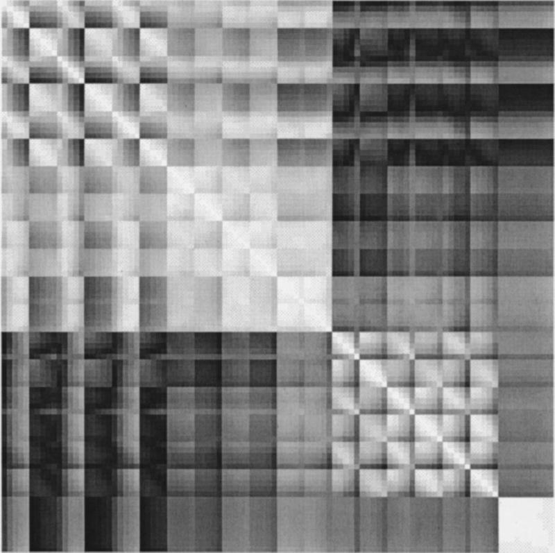
In this simulation condition, the two classes were assumed to have a multivariate Gaussian distribution with Σ = (Σ₁ + Σ₂)/2, where Σ₁ and Σ₂ were estimated from the feature samples for the malignant and benign classes. Since the feature values have different scales, their variances can vary by as much as a factor of 10⁶. Therefore, it is difficult to provide an idea about how the covariance matrix looks without listing all the entries of the 100-by-100 matrix Σ. The correlation matrix, which is normalized so that all diagonal entries are unity, is better suited for this purpose. The absolute value of the correlation matrix is shown as an image in Fig. 2. In this image, small elements of the correlation matrix are displayed as darker pixels, and the diagonal elements, which are unity, are displayed as brighter pixels. From Fig. 2, it is observed that some of the features are highly correlated or anticorrelated. The squared Mahalanobis distance was computed as Δ(∞) = 2.4, which corresponded to A_z(∞) = 0.86.

Fig. 2.

The correlation matrix for the 100-dimensional texture feature space extracted from 249 mammograms. The covariance matrix corresponding to these features was used for simulations for Case 3(a).

Case 3(b)

To determine the performance of a feature space with equivalent discrimination potential to that in Case 3(a) but with independent features, we performed an orthogonalization transformation on the SGLD features of the generated random samples used for each partitioning, as explained previously in Case 2(b).

III. RESULTS

A. Case 1: Identity covariance matrix

1. Feature selection from entire sample space

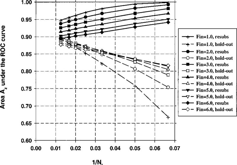
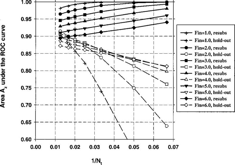
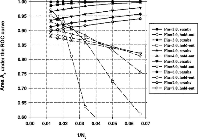
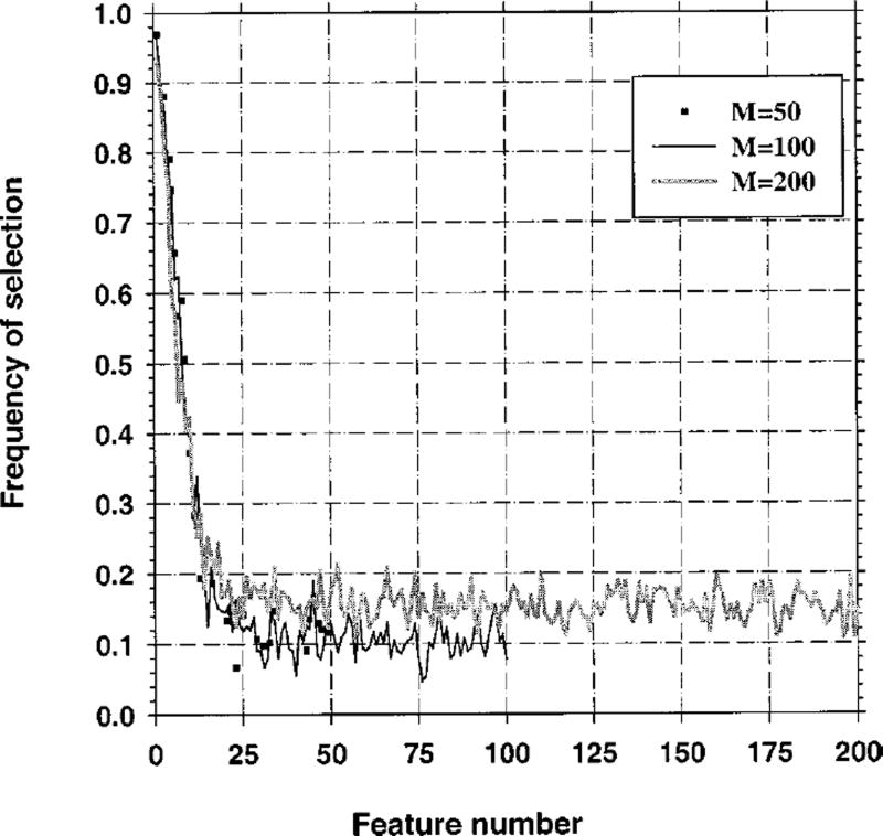
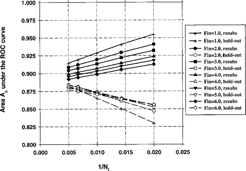
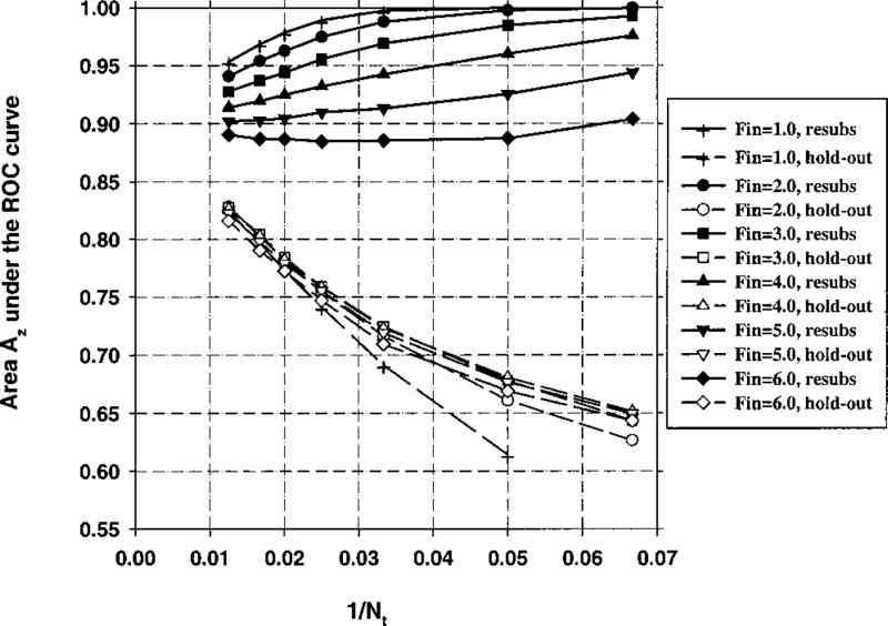
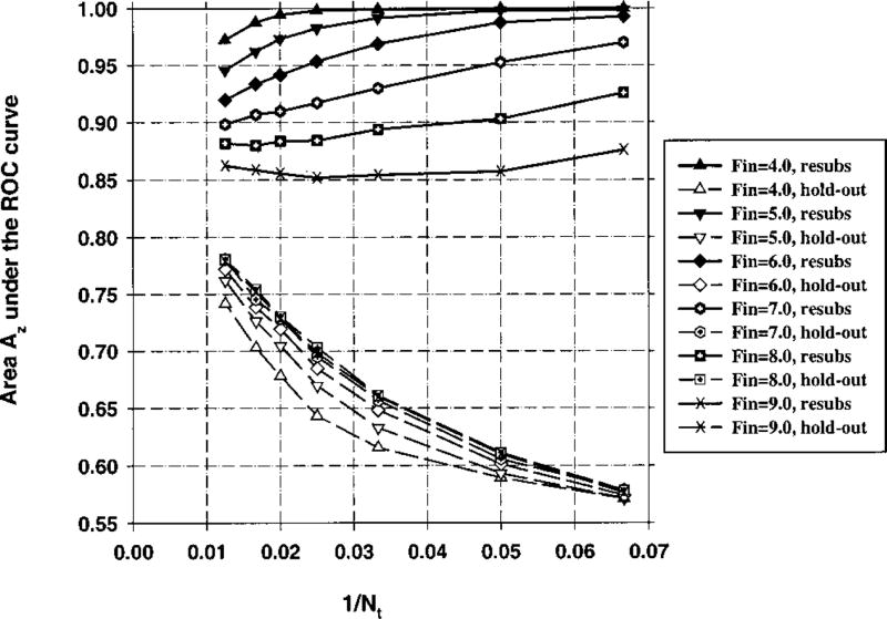
The area A_z under the ROC curve for the resubstitution and the hold-out methods is plotted as a function of 1/N_t in Fig. 3 for N_s = 100 (number of samples per class) and M = 50 (number of available features). In this figure, the F_in value in stepwise feature selection is varied between 1 and 6, and F_out=F_in−1. Figures 4 and 5 depict the relationship between A_z and 1/N_t for M = 100 and M = 200, respectively, and N_s = 100 for both cases. The average number of selected features for different values of F_in is plotted in Fig. 6. The fraction of experiments (out of a total of 50 experiments) in which feature i was selected in stepwise feature selection is plotted in Fig. 7. For the results shown in Figs. 3–7, 100 samples per class (N_s) were used in the simulation study, and the number of available features was changed from M = 50 to M = 200. In Fig. 8, we show the simulation results for a larger number of samples, N_s = 250, and M = 50.

Fig. 3.

Case 1 (identity covariance matrix), A_z(∞) = 0.89. Feature selection from the entire sample space of 100 samples/class: The area A_z under the ROC curve versus the inverse of the number of design samples N_t per class. Feature selection was performed using an input feature space of M = 50 available features.

Fig. 4.

Case 1 (identity covariance matrix), A_z(∞) = 0.89. Feature selection from the entire sample space of 100 samples/class: The area A_z under the ROC curve versus the inverse of the number of design samples N_t per class. Feature selection was performed using an input feature space of M = 100 available features.

Fig. 5.

Case 1 (identity covariance matrix), A_z(∞) = 0.89. Feature selection from the entire sample space of 100 samples/class: The area A_z under the ROC curve versus the inverse of the number of design samples N_t per class. Feature selection was performed using an input feature space of M = 200 available features.

Fig. 7.

Case 1 (identity covariance matrix), A_z(∞) = 0.89. Feature selection from the entire sample space of 100 samples/class: The frequency of feature number i, defined as the fraction of experiments in which feature i was selected. F_in = 3.0, F_out = 2.0.

Fig. 8.

Case 1 (identity covariance matrix), A_z(∞) = 0.89. Feature selection from the entire sample space of 250 samples/class: The area A_z under the ROC curve versus the inverse of the number of design samples N_t per class. Feature selection was performed using an input feature space of M = 50 available features.

2. Feature selection from training samples alone

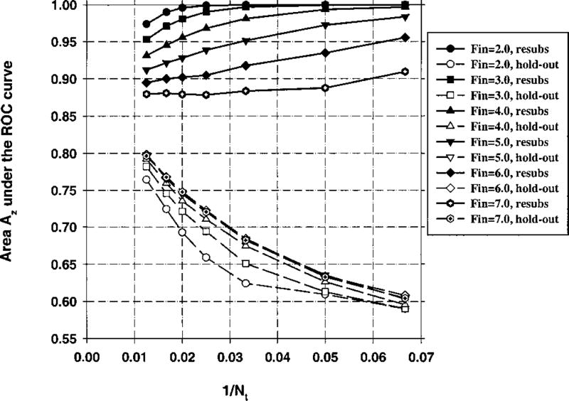
The area A_z under the ROC curve versus 1/N_t is plotted in Figs. 9–11 for M = 50, 100, and 200, respectively. In these experiments, the number of samples per class was N_s = 100. The average number of selected features changes as one moves along the abscissa of these curves. Figure 12 shows the average number of selected features for N_t = 80 per class.

Fig. 9.

Case 1 (identity covariance matrix), A_z(∞) = 0.89. Feature selection from the design samples. Total sample size N_s = 100 samples per class. The area A_z under the ROC curve versus the inverse of the number of design samples N_t per class. Feature selection was performed using an input feature space of M = 50 available features.

Fig. 11.

Case 1 (identity covariance matrix), A_z(∞) = 0.89. Feature selection from the design samples. Total sample size N_s = 100 samples per class. The area A_z under the ROC curve versus the inverse of the number of design samples N_t per class. Feature selection was performed using an input feature space of M = 200 available features.

B. Case 2: Comparison of correlated and diagonal covariance matrices

1. Feature selection from entire sample space

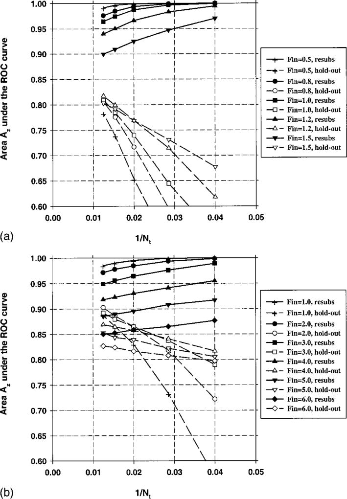
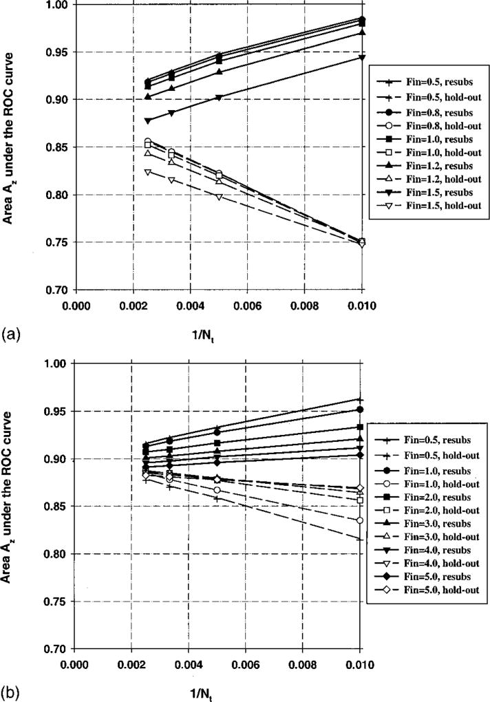
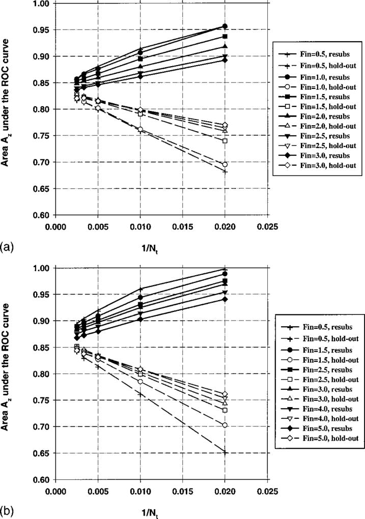
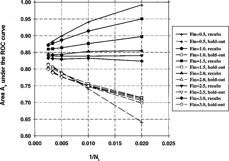
The area A_z under the ROC curve for the resubstitution and hold-out methods is plotted versus 1/N_t in Figs. 13(a) and 13(b) for Cases 2(a) and 2(b), respectively, as described in Sec. IID for N_s = 100 and M = 100. Since the individual features in Case 2(a) provide less discriminatory power than those in Case 1, the F_in value was varied between 0.5 and 1.5 in Fig. 13(a). F_out was defined as F_out=max[(F_in−1),0]. Figures 14(a) and 14(b) are the counterparts of Figs. 13(a) and 13(b), respectively, simulated with the number of samples per class N_s = 500.

Fig. 13.

(a) Case 2(a) (correlated samples, no diagonalization), A_z(∞) = 0.89. Feature selection from the entire sample space of 100 samples/class: The area A_z under the ROC curve versus the inverse of the number of design samples N_t per class. Feature selection was performed using an input feature space of M = 100 available features. (b) Case 2(b) (correlated samples, and diagonalization), A_z(∞) = 0.89. Feature selection from the entire sample space of 100 samples/class: The area A_z under the ROC curve versus the inverse of the number of design samples N_t per class. Feature selection was performed using an input feature space of M = 100 available features.

Fig. 14.

(a) Case 2(a) (correlated samples, no diagonalization), A_z(∞) = 0.89. Feature selection from the entire sample space of 500 samples/class: The area A_z under the ROC curve versus the inverse of the number of design samples N_t per class. Feature selection was performed using an input feature space of M = 100 available features. (b) Case 2(b) (correlated samples, and diagonalization), A_z(∞) = 0.89. Feature selection from the entire sample space of 500 samples/class: The area A_z under the ROC curve versus the inverse of the number of design samples N_t per class. Feature selection was performed using an input feature space of M = 100 available features.

C. Case 3: Simulation of a possible condition in CAD

1. Feature selection from entire sample space

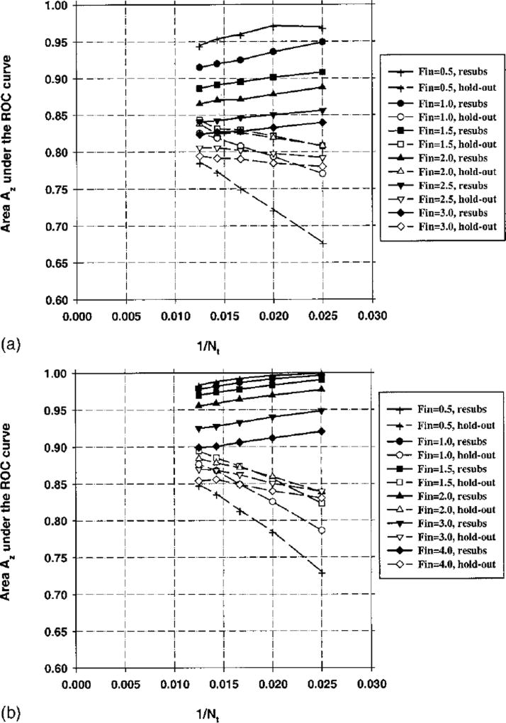
The area A_z under the ROC curve for the resubstitution and hold-out methods is plotted versus 1/N_t in Figs. 15(a) and 15(b) for Cases 3(a), and 3(b), respectively (N_s = 100 and M = 100). The F_in value was varied between 0.5 and 3.0, and F_out was defined as F_out=max[(F_in−1),0]. Figures 16(a) and 16(b) are the counterparts of Figs. 15(a) and 15(b), simulated with the number of samples per class N_s = 500.

Fig. 15.

(a) Case 3(a) (an example from CAD, no diagonalization), A_z(∞) = 0.86. Feature selection from the entire sample space of 100 samples/class: The area A_z under the ROC curve versus the inverse of the number of design samples N_t per class. Feature selection was performed using an input feature space of M = 100 available features. (b) Case 3(b) (an example from CAD, and diagonalization), A_z(∞) = 0.86. Feature selection from the entire sample space of 100 samples/class: The area A_z under the ROC curve versus the inverse of the number of design samples N_t per class. Feature selection was performed using an input feature space of M = 100 available features.

Fig. 16.

(a) Case 3(a) (an example from CAD, no diagonalization), A_z(∞) = 0.86. Feature selection from the entire sample space of 500 samples/class: The area A_z under the ROC curve versus the inverse of the number of design samples N_t per class. Feature selection was performed using an input feature space of M = 100 available features. (b) Case 3(b) (an example from CAD, and diagonalization), A_z(∞) = 0.86. Feature selection from the entire sample space of 500 samples/class: The area A_z under the ROC curve versus the inverse of the number of design samples N_t per class. Feature selection was performed using an input feature space of M = 100 available features.

2. Feature selection from training samples alone

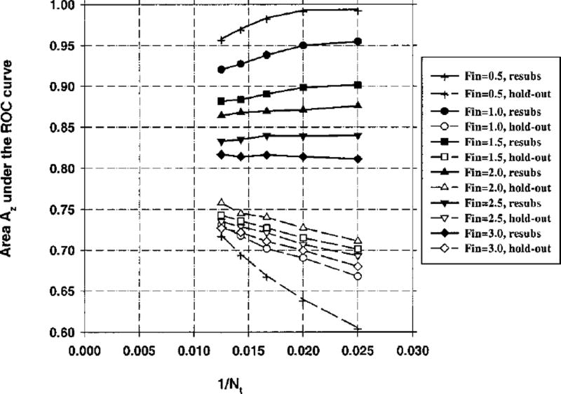
The area A_z under the ROC curve versus 1/N_t for Case 3(a) is plotted for N_s = 100 and N_s = 500 in Figs. 17 and 18, respectively.

Fig. 17.

Case 3(a) (an example from CAD, no diagonalization), A_z(∞) = 0.86. Feature selection from the design samples. Total sample size N_s = 100 samples per class. The area A_z under the ROC curve versus the inverse of the number of design samples N_t per class. Feature selection was performed using an input feature space of M = 100 available features.

Fig. 18.

Case 3(a) (an example from CAD, no diagonalization), A_z(∞) = 0.86. Feature selection from the design samples. Total sample size N_s = 500 samples per class. The area A_z under the ROC curve versus the inverse of the number of design samples N_t per class. Feature selection was performed using an input feature space of M = 100 available features.

IV. DISCUSSION

Figures 3–5 demonstrate that, in general, when the number of available samples is fixed, the bias in the mean resubstitution performance of the classifiers increases when the number of available features increases, or when the number of selected features increases. The results also reveal the potential problems with the hold-out performance when feature selection is performed using the entire sample space. The best possible hold-out performance with infinite sample size for Case 1 is A_z(∞) = 0.89. However, in Figs. 3–5, we observe that the “hold-out” estimates for large N_t values are higher than 0.89. Some of these estimates were as high as 0.97, as observed from Fig. 5. These hold-out A_z values were higher than A_z(∞) because the hold-out samples were not excluded from classifier design in the feature selection stage, but were excluded only in the second stage of classifier design, where the coefficients of the linear classifier were computed. When feature selection is performed using a small sample size, some features that are useless for the general population may appear to be useful for the classification of the small number of samples at hand. This was previously demonstrated in the literature³⁵ by comparing the probability of misclassification based on a finite sample to that based on the entire population when a certain number of features were used for classification. In our study, given a small data set, the variance in the Wilks’ lambda estimates causes some feature combinations to appear more powerful than they actually are. Recall that for Case 1, the discriminatory power of a given feature decreases with the feature number. Figure 7 demonstrates that the features numbered larger than 100, which have practically no classification capability, have more than 10% chance of being selected when F_in = 3.0 and F_out = 2.0. If training-test partitioning is performed after feature selection, and a relatively large portion of the available samples are used for training so that the estimation of linear discriminant coefficients is relatively accurate, the hold-out estimates can be optimistically biased. Figures 3–5 suggest that a larger dimensionality of the available feature space (M) may imply a larger bias. This is expected intuitively because, by using a larger number of features, one increases the chance of finding a feature that is useless but appears to be useful due to a finite sample size.

The observation made in the previous paragraph about the possible optimistic bias of the hold-out estimate when feature selection is performed using the entire sample space is not a general rule. Figures 13(a) and 15(a) show that one does not always run the risk of obtaining an optimistic bias in the hold-out estimate when the feature selection is performed using the entire sample space, even when the size of the entire sample space is small (N_s = 100) and the dimensionality of the feature space is large (M = 100). For Case 2, the best possible test performance with infinite sample size is A_z(∞) = 0.89, however, the best hold-out estimate in Fig. 13(a) is A_z = 0.82. Similarly, for Case 3, the best possible test performance with infinite sample size is A_z(∞) = 0.86, but the best hold-out estimate in Fig. 15(a) is A_z = 0.84. The features in both Cases 2(a) and 3(a) were correlated. Cases 2(b) and 3(b) were obtained from Cases 2(a) and 3(a) by applying a linear orthogonalization transformation to the features so that they become uncorrelated. Note that the linear transformation matrix is estimated from the samples used for feature selection, so it can be considered to be part of the feature selection process. Figures 13(b) and 15(b) show that after this transformation is applied, the hold-out estimates can be optimistically biased for small sample size (N_s = 100). However, in the range of small training sample size (N_t) below about 50, the orthogonalization reduces the biases and thus improves the performance estimation. This shows that performing a linear combination of features before stepwise feature selection can have a strong influence on its performance. This result is somewhat surprising, because the stepwise procedure is supposed to select a set of features whose linear combination can effectively separate the classes. One possible reason is that the orthogonalization transformation is applied to the entire feature space of M features, whereas the stepwise procedure only produces combinations of a subset of these features.

Figures 9–11, 17, and 18 demonstrate that, when feature selection is performed using the training set alone, the holdout performance estimate is pessimistically biased. The bias increases, as expected, when the number of available features is increased from M = 50 in Fig. 9 to M = 200 in Fig. 11. When a larger number of features are available, it is more likely that there will be features that appear to be more useful for the classification of training samples than they actually are for the general population. This bias reduces as the number of training samples, N_t, increases.

The biases of the hold-out performance estimates discussed above are summarized in Table I when the number of available features M = 100. When N_s = 100, Cases 1, 2(b), and 3(b) can exhibit optimistic hold-out estimates if the feature selection is performed using the entire sample space. When the number of available samples is increased to N_s = 500, we do not observe this undesired behavior, and all the hold-out performance estimates are conservative. When the feature selection is performed using the training set alone, the average hold-out performance estimate is always pessimistically biased.

Table I.

Summary of the hold-out performance bias with respect to infinite sample performance for the class distributions used in this study. Number of available samples M = 100. P: Always pessimistically biased for all F_in and F_out thresholds used in stepwise feature selection in this study; O: Could be optimistically biased for some F_in and F_out thresholds used in stepwise feature selection.

	Samples per class	Case 1	Case 2(a)	Case 2(b)	Case 3(a)	Case 3(b)
Feature selection from the entire sample space	Ns = 100	O	P	O	P	O
	Ns = 500	P	P	P	P	P
Feature selection from the design samples alone	Ns = 100	P	P	P	P	P

Figure 6 plots the number of selected features for Case 1 versus the F_in value when feature selection is performed using the entire sample space of 100 samples per class. It is observed that, for a given F_in value, the number of selected features increases when the number of available features M is increased. Figure 12 shows a similar trend between the number of selected features, the F_in value, and the number of available features when feature selection is performed using the training set alone.

When the F_in and F_out values were low, the resubstitution performance estimates were optimistically biased for all the cases studied. Low F_in and F_out values imply that many features are selected using the stepwise procedure. From previous studies, it is known that a larger number of features in classification implies larger resubstitution bias.^1,3 On the other hand, when F_in and F_out values were too high, the number of selected features could be so low that even the resubstitution estimate would be pessimistically biased, as can be observed from Fig. 14(a) (F_in = 1.5) and Fig. 15(a) (F_in = 3.0). In all of our simulations, for a given number of training samples N_t, the resubstitution estimate increased monotonically as the number of selected features were increased by decreasing F_in and F_out.

In contrast to the resubstitution estimate, the hold-out estimate for a given number of training samples did not change monotonically as F_in and F_out were decreased. This trend is apparent in Fig. 4, where the hold-out estimate at N_t = 80(1/N_t = 0.0125) is the largest for F_in = 2.0, but at N_t = 30(1/N_t = 0.033) it is next-to-smallest for the same F_in value. Another way of examining the same phenomenon is to consider different 1/N_t values on the abscissa of Fig. 4, and to observe that at different 1/N_t values, a different F_in threshold provided the best hold-out performance. In Fig. 4, the feature selection was performed using the entire sample space. A similar phenomenon can be observed in Fig. 18, where the feature selection is performed using the training samples alone. This means that for a given number of design samples, there is an optimal value for F_in and F_out (or number of selected features) that provides the highest hold-out estimate. This is the well-known peaking phenomenon described in the literature.³⁶ For a given number of training samples, increasing the number of features in the classification has two opposing effects on the hold-out performance. On the one hand, the new features may provide some new information about the two classes, which tends to increase the hold-out performance. On the other hand, the increased number of features increases the complexity of the classifier, which tends to decrease the hold-out performance. Depending on the balance between how much new information the new features provide and how much the complexity increases, the hold-out performance may increase or decrease when the number of features is increased.

For different cases studied here, the range of F_in and F_out values shown in the performance-versus-1/N_t plots was different. As mentioned in the Methods Section, F_in and F_out values for a given classification task are not known a priori, and these thresholds have to be varied over a range in order to find the best combinations of features. As mentioned in the previous paragraph, for a given number of design samples, there is an optimum value for F_in and F_out that provides the highest hold-out estimate. In this study, we aimed at finding this peak for the highest N_t in a given graph whenever possible. After this peak was found, the F_in and F_out values shown in the figures were chosen to demonstrate the performance of the classifier at each side of the peak. By examining the figures, it can be observed that the peak holdout performance was found in every case except in Fig. 5. In Fig. 5, the best hold-out performance occurs for F_in = 2.0, for which the resubstitution performance is 1.0 for all N_t values, and the hold-out performance is 0.97. Since this F_in value already shows that the hold-out performance can be too optimistic, we did not search further for the peak of the holdout performance in Fig. 5.

An interesting observation is made by examining the resubstitution performances in Figs. 9, 17, and 18, in which the feature selection is performed using the design samples alone. For F_in = 6.0 in Fig. 9, and F_in = 3.0 in Figs. 17 and 18, the resubstitution estimate increases as the number of training samples N_t increases. This may seem to contradict some previous studies in which the resubstitution estimate always decreased with increasing N_t.² However, Figs. 9, 17, and 18 are different from previous studies in that the number of selected features changes as N_t changes in these figures. The number of features selected by the stepwise procedure depends on the number of samples used for selection, which is equal to 2N_t in these figures. With an argument similar to that for the hold-out performance, there are two opposing factors that affect the resubstitution performance when N_t is increased. The first factor, which seems to be dominant, is the fact that, with large N_t, overtraining is decreased so that the resubstitution performance is reduced. The second factor, which is visible for F_in = 6.0 in Fig. 9, and F_in = 3.0 in Figs. 17 and 18, is the fact that with large N_t, the stepwise procedure selects more features, which may increase the resubstitution performance.

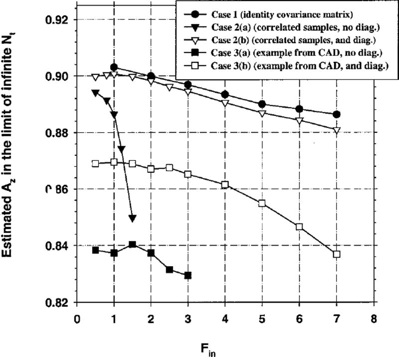
In this study, for Cases 1, 2, and 3, we investigated the classifier performance when feature selection was performed using the entire sample space, and the number of samples per class (N_s) was five times that of available features for feature selection (M). The results of these simulations are shown in Figs. 8, 14, and 16 for Cases 1, 2 and 3, respectively. Our first observation concerning these figures is that none of the hold-out estimates in these figures are higher than their respective A_z(∞) values. This suggests that it may be possible to avoid obtaining optimistic hold-out estimates by increasing the number of available samples or by decreasing the number of features used for feature selection. A second observation is that, compared to other results in this study, the relationship between the A_z values and 1/N_t is closer to a linear relation in these figures. In order to test whether the A_z(∞) value can be obtained by extrapolation as was suggested in the literature,^2,17 we performed regression analysis for the hold-out A_z estimates (versus 1/N_t) for each F_in value, and computed the y-axis intercept of the resulting regression equation. For regression analysis, we used curves obtained with N_s = 500 and M = 100 for all cases (shown in Figs. 14 and 16 for Cases 2 and 3, and not shown for Case 1). The resulting extrapolated values are shown in Fig. 19. For Case 1, we observe that the extrapolated value is within ±0.015 of the A_z(∞) value of 0.89. For Cases 2 and 3, the extrapolated values are within ±0.02 of the A_z(∞) values for small F_in ; the error increases, however, when F_in is increased. This graph suggests that when the classifier design involves feature selection, it may be possible to estimate the A_z(∞) value using the Fukunaga–Hayes method when the sample size is reasonably large. However, the error in the estimated A_z(∞) value can be large if the F_in and F_out thresholds are not chosen properly.

Fig. 19.

The estimated values of classifier accuracy in the limit of infinite training samples, obtained by fitting a linear regression to the hold-out A_z values, and finding the y-axis intercept. A_z(∞) = 0.89 for Cases 1, and 2; A_z(∞) = 0.86 for Case 3. For all cases, total sample size N_s = 500 samples per class, and number of available features M = 100.

This study examined only the bias of the mean performance estimates, which were obtained by averaging the estimates from fifty experiments as described in Sec. II D. Another important issue in classifier design and assessment is the uncertainty in the performance measure, i.e., the variance expected over replications of the experiment when a new sample of training patients and/or a new sample of test patients are drawn from the same population. The variance provides an estimate of the generalizability of the classifier performance to other design and test samples. We previously studied the components of the variance of performance estimates when the classifier is trained and tested with finite samples, but the design excludes the feature selection process.^4,5 The extension of our previous studies to include feature selection is an important further research topic.

V. CONCLUSION

In this study, we investigated the finite-sample effects on the mean performance of a linear classifier that included stepwise feature selection as a design step. We compared the resubstitution and hold-out estimates to the true classification accuracy, which is the performance of a classifier designed with the full knowledge of the population distributions. We compared the effect of partitioning the data set into training and test groups before performing feature selection with that after performing feature selection. When data partitioning was performed before feature selection, the hold-out estimate was always pessimistically biased. When partitioning was performed after feature selection, i.e., the entire sample space was used for feature selection, the hold-out estimates could be pessimistically or optimistically biased, depending on the number of features available for selection, number of available samples, and their statistical distribution. All hold-out estimates exhibited a pessimistic bias when the parameters of the simulation were obtained from correlated texture features extracted from mammograms in our previous study. The understanding of the performance of the classifier designed with different schemes will allow us to utilize a limited sample set efficiently and to avoid an overly optimistic assessment of the classifier.

Fig. 10.

Case 1 (identity covariance matrix), A_z(∞) = 0.89. Feature selection from the design samples. Total sample size N_s = 100 samples per class. The area A_z under the ROC curve versus the inverse of the number of design samples N_t per class. Feature selection was performed using an input feature space of M = 100 available features.

References

- 1.Chan H-P, Sahiner B, Wagner RF, Petrick N, Mossoba J. Effects of sample size on classifier design: Quadratic and neural network classifiers. Proc. SPIE Conf. Medical Imaging. 1997;3034:1102–1113. [Google Scholar]
- 2.Wagner RF, Chan H-P, Mossoba J, Sahiner B, Petrick N. Finite-sample effects and resampling plans: Application to linear classifiers in computer-aided diagnosis. Proc. SPIE Conf. Medical Imaging. 1997;3034:467–477. [Google Scholar]
- 3.Chan H-P, Sahiner B, Wagner RF, Petrick N. Effects of sample size on classifier design for computer-aided diagnosis. Proc. SPIE Conf. Medical Imaging. 1998;3338:845–858. [Google Scholar]
- 4.Wagner RF, Chan H-P, Mossoba J, Sahiner B, Petrick N. Components of variance in ROC analysis of CADx classifier performance. Proc. SPIE Conf. Medical Imaging. 1998;3338:859–875. [Google Scholar]
- 5.Wagner RF, Chan H-P, Sahiner B, Petrick N, Mossoba JT. Components of variance in ROC analysis of CADx classifier performance: Applications of the bootstrap. Proc. SPIE Conf. Medical Imaging. 1999;3661:523–532. [Google Scholar]
- 6.Chan H-P, Sahiner B, Wagner RF, Petrick N. Classifier design for computer-aided diagnosis: Effects of finite sample size on the mean performance of classical and neural network classifiers. Med. Phys. 1999;26:2654–2668. doi: 10.1118/1.598805. [DOI] [PubMed] [Google Scholar]
- 7.Efron B. The Jackknife, the Bootstrap, and Other Resampling Plans. Society for Industrial and Applied Mathematics; Philadelphia: 1982. [Google Scholar]
- 8.Wu C-M, Chen Y-C, Hsieh K-S. Texture feature for classification of ultrasonic liver images. IEEE Trans. Med. Imaging. 1992;11:141–152. doi: 10.1109/42.141636. [DOI] [PubMed] [Google Scholar]
- 9.Hadjiiski LM, Sahiner B, Chan H-P, Petrick N, Helvie MA. Classification of malignant and benign masses based on hybrid ART2LDA approach. IEEE Trans. Med. Imaging. 1999;18:1178–1187. doi: 10.1109/42.819327. [DOI] [PubMed] [Google Scholar]
- 10.Freeborough PA, Fox NC. MR image texture analysis applied to the diagnosis and tracking of Alzheimer’s disease. IEEE Trans. Med. Imaging. 1998;17:475–479. doi: 10.1109/42.712137. [DOI] [PubMed] [Google Scholar]
- 11.Sahiner B, Chan H-P, Petrick N, Helvie MA, Adler DD, Goodsitt MM. Computerized characterization of masses on mammograms: The rubber band straightening transform and texture analysis. Med. Phys. 1998;25:516–526. doi: 10.1118/1.598228. [DOI] [PubMed] [Google Scholar]
- 12.Garra BS, Krasner BH, Horri SC, Ascher S, Mun SK, Zeman RK. Improving the distinction between benign and malignant breast lesions: The value of sonographic texture analysis. Ultrason. Imaging. 1993;15:267–285. doi: 10.1177/016173469301500401. [DOI] [PubMed] [Google Scholar]
- 13.Gilhuijs KGA, Giger ML. Computerized analysis of breast lesions in three dimensions using dynamic magnetic-resonance imaging. Med. Phys. 1998;25:1647–1654. doi: 10.1118/1.598345. [DOI] [PubMed] [Google Scholar]
- 14.McNitt-Gray MF, Huang HK, Sayre JW. Feature selection in the pattern classification problem of digital chest radiograph segmentation. IEEE Trans. Med. Imaging. 1995;14:537–547. doi: 10.1109/42.414619. [DOI] [PubMed] [Google Scholar]
- 15.Wu Y, Giger ML, Doi K, Vyborny CJ, Schmidt RA, Metz CE. Artificial neural networks in mammography: application to decision making in the diagnosis of breast cancer. Radiology. 1993;187:81–87. doi: 10.1148/radiology.187.1.8451441. [DOI] [PubMed] [Google Scholar]
- 16.Goldberg V, Manduca A, Evert DL, Gisvold JJ, Greenleaf JF. Improvement in specificity of ultrasonography for diagnosis of breast tumors by means of artificial intelligence. Med. Phys. 1992;19:1475–1481. doi: 10.1118/1.596804. [DOI] [PubMed] [Google Scholar]
- 17.Fukunaga K, Hayes RR. Effects of sample size on classifier design. IEEE Trans. Pattern Anal. Mach. Intell. 1989;11:873–885. [Google Scholar]
- 18.Lachenbruch PA. Discriminant Analysis. Hafner; New York: 1975. [Google Scholar]
- 19.Tatsuoka MM. Multivariate Analysis, Techniques for Educational and Psychological Research. 2. Macmillan; New York: 1988. [Google Scholar]
- 20.Draper NR. Applied Regression Analysis. Wiley; New York: 1998. [Google Scholar]
- 21.Chan H-P, Wei D, Helvie MA, Sahiner B, Adler DD, Goodsitt MM, Petrick N. Computer-aided classification of mammographic masses and normal tissue: Linear discriminant analysis in texture feature space. Phys. Med. Biol. 1995;40:857–876. doi: 10.1088/0031-9155/40/5/010. [DOI] [PubMed] [Google Scholar]
- 22.Chan H-P, Sahiner B, Lam KL, Petrick N, Helvie MA, Goodsitt MM, Adler DD. Computerized analysis of mammographic microcalcifications in morphological and texture feature spaces. Med. Phys. 1998;25:2007–2019. doi: 10.1118/1.598389. [DOI] [PubMed] [Google Scholar]
- 23.Petrick N, Chan H-P, Wei D, Sahiner B, Helvie MA, Adler DD. Automated detection of breast masses on mammograms using adaptive contrast enhancement and tissue classification. Med. Phys. 1996;23:1685–1696. doi: 10.1118/1.597756. [DOI] [PubMed] [Google Scholar]
- 24.Norusis MJ. SPSS for Windows Release 6 Professional Statistics. SPSS Inc.; Chicago, IL: 1993. [Google Scholar]
- 25.Peterson WW, Birdsall TG, Fox WC. The theory of signal detectability. Trans. IRE Prof. Grp. Inform. Theory PGIT-4. 1954:171–212. [Google Scholar]
- 26.Tanner WP, Swets JA. A decision-making theory of visual detection. Psychol. Rev. 1954;61:401–409. doi: 10.1037/h0058700. [DOI] [PubMed] [Google Scholar]
- 27.Green DM, Swets JA. Signal Detection Theory and Psychophysics. Wiley; New York: 1966. [Google Scholar]
- 28.Swets JA. ROC analysis applied to the evaluation of medical imaging techniques. Invest. Radiol. 1979;14:109–121. doi: 10.1097/00004424-197903000-00002. [DOI] [PubMed] [Google Scholar]
- 29.Hanley J, McNeil B. The meaning and use of the area under a receiver operating characteristic (ROC) curve. Radiology. 1982;143:29–36. doi: 10.1148/radiology.143.1.7063747. [DOI] [PubMed] [Google Scholar]
- 30.Metz CE. ROC methodology in radiologic imaging. Invest. Radiol. 1986;21:720–733. doi: 10.1097/00004424-198609000-00009. [DOI] [PubMed] [Google Scholar]
- 31.Simpson AJ, Fitter MJ. What is the best index of detectability. Psychol. Bull. 1973:80. [Google Scholar]
- 32.Metz CE, Herman BA, Shen J-H. Maximum likelihood estimation of receiver operating characteristic (ROC) curves from continuously-distributed data. Statistics in Medicine. 1998;17:1033–1053. doi: 10.1002/(sici)1097-0258(19980515)17:9<1033::aid-sim784>3.0.co;2-z. [DOI] [PubMed] [Google Scholar]
- 33.Dorfman D, Alf E. Maximum likelihood estimation of parameters of signal detection theory and determination of confidence intervals-rating method data. J. Math. Psychol. 1969;6:487. [Google Scholar]
- 34.Haralick RM, Shanmugam K, Dinstein I. Texture features for image classification. IEEE Trans. Syst. Man Cybern. SMC-3. 1973:610–621. [Google Scholar]
- 35.Raudys SJ, Jain AK. Small sample size effects in statistical pattern recognition: Recommendations for practitioners. IEEE Trans. Pattern Anal. Mach. Intell. 1991;13:252–264. [Google Scholar]
- 36.Hughes GF. On the mean accuracy of statistical pattern recognizers. IEEE Trans. Inf. Theory. 1968;14:55–63. [Google Scholar]