Deep Auto-context Convolutional Neural Networks for Standard-Dose PET Image Estimation from Low-Dose PET/MRI

Abstract

Positron emission tomography (PET) is an essential technique in many clinical applications such as tumor detection and brain disorder diagnosis. In order to obtain high-quality PET images, a standard-dose radioactive tracer is needed, which inevitably causes the risk of radiation exposure damage. For reducing the patient’s exposure to radiation and maintaining the high quality of PET images, in this paper, we propose a deep learning architecture to estimate the high-quality standard-dose PET (SPET) image from the combination of the low-quality low-dose PET (LPET) image and the accompanying T1-weighted acquisition from magnetic resonance imaging (MRI). Specifically, we adapt the convolutional neural network (CNN) to account for the two channel inputs of LPET and T1, and directly learn the end-to-end mapping between the inputs and the SPET output. Then, we integrate multiple CNN modules following the auto-context strategy, such that the tentatively estimated SPET of an early CNN can be iteratively refined by subsequent CNNs. Validations on real human brain PET/MRI data show that our proposed method can provide competitive estimation quality of the PET images, compared to the state-of-the-art methods. Meanwhile, our method is highly efficient to test on a new subject, e.g., spending ~2 seconds for estimating an entire SPET image in contrast to ~16 minutes by the state-of-the-art method. The results above demonstrate the potential of our method in real clinical applications.

1. Introduction

Positron emission tomography (PET) is a functional imaging technique, which produces 3D in-vivo observation of the metabolic process in the body. It provides molecular information on the biology of many diseases. Accordingly, PET has been increasingly recognized as an important tool for diagnosis [1, 2], determination of prognosis [3, 4], and response monitoring in oncology [5, 6]. There are also other imaging technologies, such as computed tomography (CT) and magnetic resonance imaging (MRI). Recently the introduction of PET/CT and PET/MRI scanners enables the acquisition of both structural and functional information in a single scan session.

The high-quality PET images play a crucial role in diagnosing brain diseases and disorders [7], because they can provide detailed functional information for assessment and diagnosis. In order to obtain the high-quality PET images, a standard-dose tracer injection to tissue or organ is needed, which inevitably raises the risk of radioactive exposure. To address this problem, the well-known As Low As Reasonably Achievable (ALARA) [8] principle is adopted to minimize the radiation exposure in clinical practice. Although the principle helps to decrease the risk of radiation exposure, it also degrades the quality of PET images and potentially involves unnecessary noises and artifacts. Two examples of the low-dose PET (LPET) and their corresponding standard-dose PET (SPET) images are shown in Fig. 1. It can be observed that the quality of the LPET images is worse than that of the SPET images.

Fig. 1.

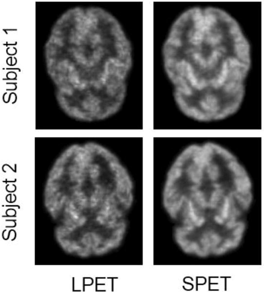
Two examples of the LPET images and their corresponding SPET images.

In order to improve the quality of the acquired PET images, numerous reconstruction and denoising methods have been developed. Mejia et al. [9] proposed a multi-resolution approach for noise reduction of PET images by employing specific filters to homogeneous and heterogeneous image regions. Pogam et al. [10] succeeded in addressing the issue of resolution loss with standard denoising by combining the complementary wavelet and curvelet transforms. Bagci et al. [11] used the singular value thresholding concept and the Stein‟s unbiased risk estimation method to optimize the soft thresholding rule for denoising. These techniques are mainly designed for SPET images only. However, our objective here is to estimate the SPET image from the corresponding LPET image, which is acquired with low-dose tracer injection. Similar works can be found for the quality enhancement of CT images. For example, Alban et al. [12] proposed an adaptive iterative dose reduction (AIDR) method to achieve the high-quality images, while reducing the radiation dose in CT acquisition.

Multi-modality data has been proven to provide complementary and effective information for increasing the quality of each single modality [13, 14]. It is shown in the literature that the anatomical or the structural information (e.g., from CT or MRI [15, 16]) contributes to better SPET image quality. In our work, we utilize both the LPET images and the corresponding structural T1 images for the estimation of the high-quality SPET images. We will detail the way to combine T1 images and LPET images using convolutional neural network (CNN) to estimate SPET images in Section 3.1.

In this paper, we first use a basic four-layer CNN to build a relatively simple model, which derives the SPET image from the LPET image and the T1 image. As an end-to-end architecture, the deep network maps the LPET and the T1 inputs to the SPET output directly without using handcrafted features. Then, we treat the tentatively estimated SPET image as the source of the context information [17]. In addition to the context information, both original LPET and T1 images are also used as inputs to a new four-layer CNN. In this way, we gradually concatenate multiple CNNs into a much deeper network. The entire network, which consists of multiple four-layer CNNs, can be optimized altogether with back-propagation. The experimental results reveal that the proposed method can effectively utilize the structural information in T1 image for the estimation of the high-quality SPET image. Meanwhile, the auto-context [18] strategy allows us to gradually improve the quality of the SPET estimation, given multiple four-layer basic CNNs. In general, our method achieves competitive performance regarding the quality of the estimated SPET images while its time cost is significantly reduced compared to the state-of-the-art methods.

The rest of this paper is organized as follows. We will review the related work in Section 2, and then describe the details of our proposed method in Section 3. Section 4 quantitatively analyzes key components of the proposed method and conducts comparisons with the state-of-the-art methods. The conclusions are drawn in Section 5.

2. Related Work

Research efforts have been made in the literature to directly estimate the SPET images from the LPET images. The estimation often requires the input of the tracer-free MRI scan and relies on the sparse learning technique. For example, in [14], the mapping-based sparse representation (m-SR) was adopted for SPET image reconstruction. To speed up the process, the patch-selection-based dictionary construction method was used to build a relatively small but representative dictionary, which can heavily reduce the processing time. Subsequently, a semi-supervised tripled dictionary learning method was used for SPET image reconstruction [19]. This method can improve the prediction results by utilizing multiple modalities (i.e., T1 image, fractional diffusivity and mean diffusivity from diffusion weighted data). It also allows a certain modality to be missing, thus including huge clinical data for training. Recently, An et al. [20] proposed the data-driven multilevel canonical correlation analysis (MCCA) scheme to map the SPET and the LPET image data into a common space, where the patch-based sparse representation was then utilized to generate the coupled LPET and SPET dictionaries. These sparse-learning-based methods consist of several steps generally, including patch extraction, encoding, and reconstruction. Most of these methods are time-consuming particularly when testing new cases, which have to solve a large number of optimization problems and thus might not be applicable in real clinical practice.

CNN dates back to decades [21], and deep CNNs have shown an explosive popularity partially due to its success in image classification tasks [22, 23]. This technique has been successfully applied to many computer vision fields, such as face detection [24–26], semantic segmentation [27, 28], and object tracking [29–31]. There are also some successful applications in medical image fields, such as cell detection [32, 33] and prostate segmentation [34, 35]. There are several factors that lead to its success: (i) the efficient implementation on modern powerful GPUs to train large networks with huge number of parameters [23], (ii) the proposal of useful tricks like Rectified Linear Unit (ReLU) [36] and dropout [37] that avoid the problems of gradient vanish and overfitting, and (iii) an abundance of labeled data (like ImageNet [38]) for training deep architectures. Recently, the proposed mechanism called batch normalization [39] also helps to speed up convergence in training very deep neural networks, leading to better performance. Specifically, Li et al. [40] proposed a deep-learning-based imaging data completion method to predict PET image from structural MRI image. Our method differs from this method in two ways. First, we apply deep neural network to estimate SPET by using multiple modalities, i.e., LPET and T1 images. Second, compared to [40], which has only three convolution layers, our network is much deeper and effectively leverage the auto-context information for the purpose of SPET estimation.

Recently, Dong et al. [41] presented a method namely Super-Resolution Convolutional Neural Network (SRCNN) for single image super-resolution, which directly learns an end-to-end mapping between low-resolution and high-resolution images. This model, which takes the low-resolution image as input and outputs the high-resolution one, partly inspired our work for SPET image estimation from the LPET image. However, different from Dong’s work, we propose to incorporate the structural T1 image in the input layer of the CNN architecture, and refine the estimation of the SPET image iteratively in an auto-context way based on the inputs of multiple modalities, which makes our model much deeper compared to Dong’s model.

3. Method

We present the details of our deep CNNs for SPET estimation in this section. We first introduce the basic multi-modal CNN, which maps the inputs of LPET and T1 to the output of SPET within four convolution layers only. Then, we concatenate multiple basic CNN modules into a deeper network following the auto-context fashion, such that the tentative SPET estimation can be iteratively refined with the help of the context information and the original LPET/T1 input images.

3.1 The Basic Multimodality CNN Architecture

In this work, we propose to use the CNN model for estimating the SPET image from LPET and T1 images. Our work is motivated by the fact that, in addition to the low-quality functional data, structural T1 images can help the estimation of the high-quality functional images. Although CNNs have been used for similar tasks in the literature, it is still challenging to fuse multiple medical image modalities. To this end, we treat multimodality images as different feature maps, and input them to CNN after concatenation. In this way, we present a straightforward solution for combining multi-modality image data. Since T1 image contains complementary information other than the functional PET data, our CNN architecture is capable of better estimating SPET from LPET and T1 images.

Considering the limited number of training images, we switch to solve the problem slice by slice here. That is, we extract all axial slices and treat them as separate images independently in training. For a new test subject, we estimate all slices and then stack them into the 3D volume along the inferior-superior direction. Our experiments confirm that the final results are observably satisfactory along the inferior-superior direction, as shown in Fig. 9.

Fig. 9.

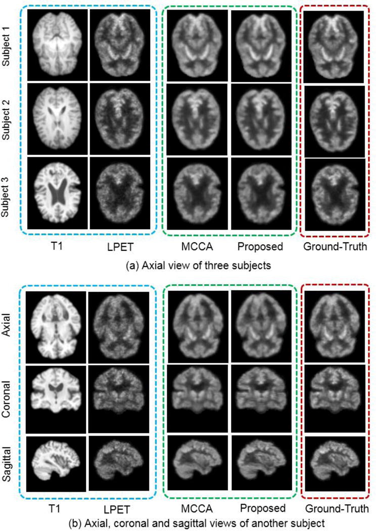
Visual comparisons of our method and the MCCA method. Each row of (a) shows a subject from the axial view. (b) shows another subject from the axial, coronal and sagittal views, respectively. ‘T1′ represents the input T1 image, and ‘LPET’ represents the input LPET image. ‘MCCA’ represents the SPET image estimated by the MCCA method. The last column represents the ground-truth SPET images.

The multimodality CNN, whose architecture is shown in Fig. 2, aims to learn the end-to-end mapping between the input LPET and T1 images and the output SPET image. Note that there are two input feature maps of this CNN in the input layer, corresponding to T1 image and LPET image, respectively. The network consists of four convolution layers, without using any pooling. The main reason is that pooling is commonly used in recognition and classification for reducing the dimension of feature maps and also making the network invariant to small translation of the input. Therefore, pooling might not be suitable for pixel-wise image quality enhancement in this work. On the other hand, the convolution layers provide similar functions regarding sparse coding, including patch extraction and representation, non-linear mapping, and reconstruction [42].

Fig. 2.

The architecture of the basic four-layer CNN used to estimate SPET from LPET and T1 images. The inputs include two feature maps corresponding to LPET and T1 image patches, respectively. The output is the corresponding SPET image patch. There are four convolution layers in this basic CNN model.

In our basic multimodality CNN model, we concatenate the two patches of LPET and T1 in the input layer, followed by four convolution layers. The first convolution layer contains n₁ filters of the support m × f₁ × f₁, where m is the number of the feature maps (with m = 2 here), and f₁ × f₁ denotes the spatial size of the filter. In general, the first layer can be expressed as

$$max(0,W_1\ast [Y,Z]+B_1),$$ (1)

where * represents the convolutional operator, Y and Z denote the LPET and T1 image patches respectively, and [, ] means the concatenation operation that combines two patches. W₁ and B₁ denote the filters and the biases, respectively. Intuitively, W₁ applies n₁ convolution filters on the input image patches, each of which has a kernel size of m×f₁×f₁. The output thus consists of n₁ feature maps.

The second, third, and fourth convolution layers can be configured in the similar way. For example, we set the second convolution layer to contain n₂ filters of the size n₁ × f₂ × f₂. So the parameters of the second layer can be represented as W₂ and B₂. After the second convolution layer, we will get n₂ feature maps as the output. Eventually, in the fourth convolution layer, there is only one filter (n₄ = 1). The single output of the fourth layer corresponds to the expected output of the SPET image patch, which shares the same center location with the input LPET and T1 image patches. All other parameters of individual layers are shown in Fig. 2. In particular, we set m = 2, n₁ = n₂=n₃ = 64, and f₁ = f₂ = f₃ = 3. We do not use any padding in each convolution layer, so the sizes of the feature maps decrease when the layer becomes deeper. For example, as shown in Fig. 2, the original size of the input LPET in training is 27 × 27, and the size of the output is 19 × 19.

Let us denote the output image estimated by the basic four-layer CNN as F_basic(Y_i, Z_i; θ_basic). Here, F indicates the end-to-end mapping, and θ_basic = {W₁,W₂,W₃,W₄,B₁,B₂,B₃,B₄} records the estimated network parameters. We term X_i as the ground-truth SPET for the i-th training subject image patch. The input LPET and T1 image patches are denoted as Y_i and Z_i, respectively. θ_basic can thus be solved by minimizing the error between the reconstructed output F_basic(Y_i,Z_i;θ_basic) and the corresponding ground-truth X_i of the same size with that of the output for training. We use the Mean Squared Error (MSE) as the loss function:

$$L_{\mathit{\text{basic}}}({\theta }_{\mathit{\text{basic}}})=\frac{1}{M}{\displaystyle \sum _{i=1}^M\Vert F(Y_i},Z_i;{\theta }_{\mathit{\text{basic}}})-X_i{\Vert }^2,$$ (2)

where M is the number of the training image patches. We use stochastic gradient descent with the standard back-propagation [43] to minimize the loss function. Using the L₂ loss function favors a high Peak Signal to Noise Ratio (PSNR). Note that PSNR is a widely used metric for quantitatively evaluating image restoration quality, as it is related to the perceptual quality. Our goal is to make the estimated SPET and the ground- truth SPET as similar as possible.

Note that the input/output sizes shown in Fig. 2 apply to the training process only. In testing, we treat the trained CNN model as fully convolutional network (FCN) [41] which can take the entire LPET and T1 images as inputs. This operation avoids to apply CNN for each patch independently and can save large computational cost. Since there is no padding in each convolution layer, we apply zero padding to the input test image to make sure that the sizes of the input image and the final output image are the same. For example, if the size of the input test image is 100 × 100 and it intends to pass four convolution layers of many 3×3 filters, we pad the input image and augment its size to 108 × 108 prior to the first convolution layer. In this way, the final output image will reduce to the size of 100 × 100.

Meanwhile, batch normalization was recently introduced by Ioffe et al. [39] to ease the training of deep neural networks. It reflects the fact that neural networks tend to learn more efficiently when their inputs are normalized to zero mean with unit variance. This strategy can be extended to the internal layer of CNNs. To this end, we apply batch normalization for every convolution layer in our implementation. For each convolution layer in Fig. 2, the output from the precedent layer can thus be processed through batch normalization and then feed as the input to the subsequent convolution layer.

3.2 Deep Auto-Context CNNs for SPET Estimation

We propose to concatenate multiple CNNs to formulate a much deeper structure, to improve the quality of the estimated SPET image gradually. The concatenated CNNs, which are shown in Fig. 3, lead to a deep auto-context-like learning architecture [17, 18]. First, we use the basic four-layer CNN (shown in Fig. 2) to estimate the SPET image based on both LPET and T1 images. Then, the tentatively estimated SPET, along with the original LPET and T1 images, are all input to the subsequent new four -layer CNN. That is, there are three input channels for the second and latter CNNs, i.e., the tentatively estimated SPET, LPET, and T1 images.

Fig. 3.

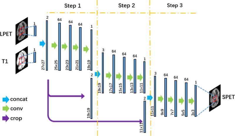
Illustration of the deep auto-context CNN architecture. ‘Concat’ represents concatenation operation that concatenates individual feature maps. ‘Conv’ represents the convolutional operation. ‘Crop’ represents the crop operation that keeps the sizes of different feature maps consistent. In Step 1, the inputs of the basic four-layer CNN are LPET and T1 images. In Step 2 and Step 3, the tentatively estimated SPET image from the last step is also included as an additional input.

In our implementation, we concatenate three four-layer CNNs to formulate the deep structure. The output of the 1^st CNN (namely after “Step 1”) is combined with the original LPET and T1 images, which are cropped from the center to get the same size with the output of CNN 1. The 2^nd (Step 2) and the 3^rd (Step 3) CNNs share the same architecture with Step 1, though the numbers of the input feature maps vary slightly as in Fig. 3. The sizes of the outputs of the 2^nd and the 3^rd CNNs are 11×11 and 3×3 in training, respectively.

With three four-layer CNNs concatenated in our implementation, there are totally 12 convolution layers, which make our architecture deep enough to estimate SPET from LPET and T1. Note that our deep architecture is significantly different from the conventional 12-layer convolutional neural network. Specifically, the LPET and T1 image inputs are forcefully directed to Step 2 and Step 3 in our method. Concerning the high similarity between LPET and SPET, the estimation of SPET can easily be dominated by LPET while ignoring T1 image. Meanwhile, the learning may end within a few convolution layers (e.g., only four layers in Step 1) as the mapping from LPET to SPET is not complex. With concatenated CNNs, T1 images are directly used as the inputs of each step and thus can play a more important role in the estimation of SPET even though its appearance is very different from SPET (compared with LPET especially). The influence of the structural information from T1 now can arrive at the very deep layers in our architecture through the concatenated CNNs. For fair comparison, in Section 4.4, we will conduct experiments with the conventional 12-layer CNN, where our method clearly shows better SPET estimation capability than simply increasing the number of layers in CNN.

The concatenation of CNNs also leads to auto-context-like learning [18]. Specifically, the tentative estimation of each four-layer CNN (e.g., Step 1) can be further refined with the subsequent CNNs (e.g., Step 2). Moreover, the parameters of the concatenated CNNs can be optimized jointly with back-propagation. This differs from the conventional auto-context learning framework where the concatenated classifiers/regressors are often trained independently. In the final, we formulate the entire architecture of the concatenatd CNNs into an end-to-end mapping, which estimates SPET from the combination of LPET and T1 images directly.

It is worth noting that direct training of the convolutional network with such a large depth may easily fall into local minima. Inspired by previous studies on training neural networks with deep supervision [44, 45], the weighted auxiliary loss is also adopted in the network to further strengthen the training process. In particular, the auxiliary loss is computed from the end of each step. We derive from (2) the loss after Step i and denote it as L_i. The total loss L_total for the entire deep auto-context CNN architecture is:

$$L_{\mathit{\text{total}}}({\theta }_{\mathit{\text{total}}})=\beta (L_1+L_2)+L_3+\phi ({\theta }_{\mathit{\text{total}}})$$ (3)

where φ(θ_total) is the L₂-norm regularization term upon the estimated network parameters. In our experiments, β is adopted to balance the auxiliary losses among individual steps. Note that the term X_i in Eq. (2) varies for different steps when computing the auxiliary loss. We compute the loss for each step as the mean squared error between the estimated SPET and the ground-truth SPET. To this end, we need to crop the ground-truth SPET, such that it has the same size as the estimated SPET patch in each step. For example, the ground-truth SPET is cropped to 19×19 in Step 1, then 11×11 in Step 2, and 3×3 in Step 3.

4 Experimental Results

We first introduce the dataset used in the experiments and discuss the parameter settings (Sections 4.1–4.2). After that, we investigate the impact of using the structural information (i.e., T1 images) for the estimation of the functional SPET data (Section 4.3). Next, we explore how our proposed deep auto-context CNNs gradually refine the SPET estimation by concatenating multiple CNNs (Section 4.4). Finally, we compare the proposed method with state-of-the-art method to demonstrate its effectiveness (Section 4.5).

4.1 Dataset

Our dataset contains 16 subjects, each of which has LPET, SPET, and T1 images. All data were acquired on a Siemens Biograph mRI PET-MR system. Their demographic information is summarized in Table 1. This study is approved by the University of North Carolina at Chapel Hill Institutional Review Board.

Table 1.

Demographic information of the subjects in the experiments.

Subject ID	Age	Gender	Weight (kg)
1	26	Female	50.3
2	30	Male	137.9
3	33	Female	103.0
4	25	Male	85.7
5	18	Male	59.9
6	19	Female	72.6
7	36	Female	102.1
8	28	Male	83.9
9	65	Female	68.0
10	86	Male	68.9
11	86	Female	74.8
12	66	Female	58.9
13	61	Male	83.9
14	81	Male	106.5
15	70	Female	61.2
16	72	Female	77.1

Before the PET scanning, each subject is administered an average of 203 MBq (from 191 MBq to 229 MBq) of ¹⁸F-2-deoxyglucose (¹⁸FDG). During PET scanning, an SPET image is obtained in a 12-minute period within one hour of tracer injection, based on standard imaging protocols. The LPET scans are acquired in a three-minute short period, with standard-dose tracer injection, to simulate the acquisition at a reduced dose of radioactive trace. The simulation is equivalent to a quarter of the standard dose. The SPET and LPET images are acquired separately, so the noises in SPET and LPET are not correlated. All PET scans are reconstructed using standard methods from the vendor. Attenuation correction, scatter and scanner uniformity are included using the vendor‟s standard procedure. Each PET image has a voxel size of 2.09× 2.09 × 2.09mm³. Meanwhile, the T1-weighted MPRAGE image is acquired with 1 × 1 × 1mm³ resolution. For each subject, the T1 image is linearly aligned onto the corresponding PET image via affine transformation [46], followed by skull stripping [47] and intensity normalization. All images are further aligned to the space of a selected subject using FLIRT [48]. At last, we crop each image to the size of 120 × 100 × 100 voxels to remove the redundant background.

4.2 Experimental Configuration

The leave-one-out cross-validation strategy is employed for evaluation. That is, each time one subject is used for testing and the other images are for training. In this paper, CAFFE [49] is used to implement the CNN architecture. In the training phase, we use the same strategy with [42] that randomly selects 30,000 patches from each training image. There are totally 4.5 × 10⁵ training patches in every leave-one-out case. The size of each patch is defined as 27 ×27. In Step 1, the filter sizes of the four convolution layers are set to 3 × 3, and the size of the output patch after Step 1 is thus 19 × 19. The numbers of the filters of the initial three convolution layers are the same, n₁ = n₂ = n₃ = 64, while there is only one filter, n₄ = 1, in the last layer of Step 1. Step 2 and Step 3 share similar parameters with Step 1, though their feature map sizes vary as in Fig. 3. The learning rates are 1 × 10⁻⁴ for Step 1 and Step 2, and 1 × 10⁻⁵ for Step 3. A smaller learning rate in the last four-layer CNN (i.e., Step 3) is helpful to the convergence of the network in training [50]. We adopt “SGD” as the solver for the simultaneous optimization of all steps in back-propagation. Although we use a fixed patch size in training, the deep networks can be applied to images of arbitrary sizes during testing.

To evaluate the performance of the proposed method quantitatively, we use the normalized mean squared error (NMSE) in (4) and the peak signal-to-noise ratio (PSNR) in (5):

$$\mathit{\text{NMSE}}=\frac{\Vert X-\widehat{X}|{|}_2^2}{\Vert X{\Vert }^2},$$ (4)

$$\mathit{\text{PSNR}}=10\text{ln}\left(\frac{N{D}^2}{\Vert X-\widehat{X}{\Vert }_2^2}\right),$$ (5)

where X is the ground-truth SPET image, $\widehat{X}$ is the estimated SPET image, D is the intensity range of image X, and N represents the total number of voxels in the image. Lower NMSE and higher PSNR indicate better quality of the estimated SPET.

4.3 Contribution of T1 in Estimating SPET, using Basic 4-Layer CNN

To demonstrate the effectiveness of integrating multimodality data for the estimation of SPET, we compare the performances achieved by using LPET input only and by using the combination of LPET and T1 images. When dealing with the single LPET input, we employ the same setting as in Fig. 2, but the input layer only considers the LPET image. The performances achieved by using different input settings are shown in Fig. 4. As we use the leave-one-out strategy, each subject is chosen for testing in turn. ‘LPET’ indicates the PSNR/NMSE scores by comparing the input LPET image with the ground-truth SPET image directly. ‘Estimation by LPET’ represents the estimation SPET results when using LPET as the input for our basic four-layer CNN only. ‘Estimation by LPET+T1′ represents the estimation SPET results when using the combined inputs of LPET and T1 as in Fig. 2.

Fig. 4.

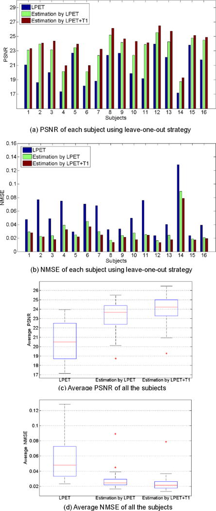
The performances of using different input image settings, measured by PSNR and NMSE. (a) and (b) give the PSNR and NMSE scores of each subject in the leave-one-out validation. (c) and (d) give the average PSNR and NMSE scores of all the subjects. ‘LPET’ indicates the PSNR/NMSE between the original LPET and the ground-truth SPET. ‘Estimation by LPET’ represents the scores of the results estimated using only LPET as the input. ‘Estimation by LPET+T1′ represents the scores of the results estimated using both LPET and T1 images.

We can observe that the results of ‘Estimation by LPET’ are worse than ‘Estimation by LPET+T1′. In particular, the average PSNR scores of ‘Estimation by LPET’ and ‘Estimation by LPET+T1′ are 23.11 and 23.85, respectively. And the average NMSE scores of ‘Estimation by LPET’ and ‘Estimation by LPET+T1′ are 0.0299 and 0.0254, respectively. The PSNR scores and the NMSE scores are significantly different between ‘Estimation by LPET’ and ‘Estimation by LPET+T1′ (p-value<0.01 in paired t-test). The results above imply that the structural information from T1 yields important cues for estimating the high-quality functional SPET, even though structural T1 differs from PET significantly regarding their appearances. We also provide two examples (corresponding to two rows) in Fig. 5 for visual observation, where our method yields more satisfactory estimation results regarding the ground-truth.

Fig. 5.

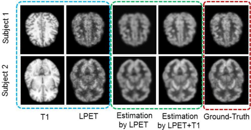
Visual examples of using multimodality inputs for SPET estimation. The two rows represent two different subjects. Original inputs of the LPET and the T1 images are in the blue dashed box. The estimated SPET images using different input settings are in the green dashed box. The ground-truth SPET images are in the red dashed box. ‘T1′ represents the input T1 image. ‘LPET’ is for the input LPET image. ‘Estimation by LPET’ represents the estimated SPET image by using only LPET as the input. ‘Estimation by LPET+T1′ represents the estimated SPET by using both LPET and T1 images as the inputs. ‘Ground-Truth’ is for the SPET image acquired in our dataset.

4.4 Concatenation of Basic CNNs

Different from simply increasing the number of the layers in conventional CNN, we follow the auto-context strategy and concatenate three 4-layer basic CNNs in this work. Both LPET and T1 image patches, as well as the tentatively estimated SPET (if available), are used as the inputs to each of the three CNNs. In order to evaluate the effectiveness of concatenating multiple CNNs for auto-context-like estimation of SPET, we show the performances (measured by PSNR/NMSE) after individual steps of CNNs in Fig. 6. The average PSNR scores after Steps 1, 2, and 3 are 23.85, 24.55 and 24.76, respectively. The average NMSE scores after Steps 1, 2, and 3 are 0.0254, 0.0215 and 0.0205, respectively. The t-tests also yield p-values that are lower than 0.01 when comparing the resulted PSNRs and NMSEs between Step 2 and Step 1, and between Step 3 and Step 2. These results reveal that the estimation quality improves greatly after refining the output of Step 1 in Step 2. The improvement of the overall PSNR/NMSE score becomes relatively limited when Step 3 is applied. To this end, we argue that the concatenation of multiple CNNs is effective to improve the quality of the estimated SPET. However, too many steps would increase the complexity of the entire network significantly, which could come with higher difficulty and more time cost for training. We have concatenated more CNNs but this fails to yield better performance. In general, we choose to concatenate three four-layer CNNs, considering both the performance and the computational efficiency.

Fig. 6.

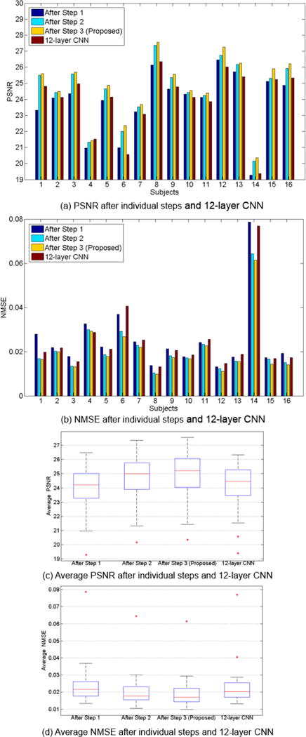
The performances of concatenating multiple basic CNNs, in terms of PSNR and NMSE. (a) and (b) give the PSNR and NMSE scores of each subject by using the leave-one-out validation. (c) and (d) give the average PSNR and NMSE scores of all the subjects. Note that our method concatenates three basic CNNs, which is also indicated by ‘After Step 3′ in this figure. The results of the conventional 12-layer CNN are also shown in the figure.

In order to further reveal the power of our proposed method, here we compare our deep auto-context architecture (12 layers in total) with the 12-layer conventional CNN model. The results are also shown in Fig. 6. We can see that our model outperforms the 12-layer CNN. The average PSNR scores of our proposed method and the 12-layer CNN are 24.76 and 23.98, respectively. The average NMSE scores of our proposed method and the 12-layer CNN are 0.0206 and 0.0247, respectively. The differences between our method and the 12-layer CNN are statistically significant. These results show that, by concatenating multiple CNNs and forcefully directing information flows, the auto-context-like network is more effective than simply increasing the number of layers in the conventional CNN.

We concatenate multiple CNNs and build a deep structure, the training of which may become challenging. Therefore, we adopt the batch normalization strategy in modeling the network. In Fig. 7, we plot the changes of the training losses with respect to the number of iterations during training. The comparisons are conducted between the proposed method and the conventional 12-layer CNN, with and without batch normalization. Clearly, the strategy of batch normalization greatly contributes to the convergence of training. For example, without batch normalization, the conventional 12-layer CNN can hardly be trained. Meanwhile, we note that, with directed data flow in our concatenated CNNs, the training process can converge faster than the conventional CNN (i.e., by comparing the red and the green curves). The observation confirms that our method can effectively model the estimation of SPET from LPET and T1.

Fig. 7.

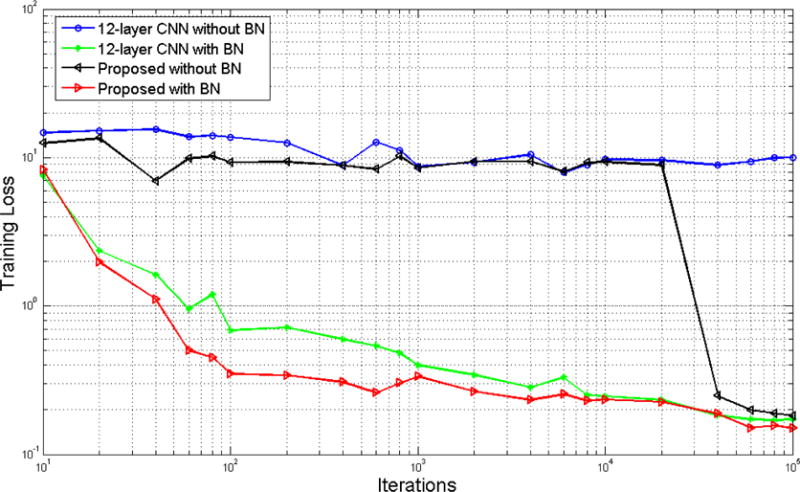
Training loss with respect to the number of iterations for the 12-layer CNN and our proposed deep CNN architecture, with and without batch normalization.

4.5 Comparison with Sparse-Learning-Based MCCA Method

We also compare our method with state-of-the-art MCCA method [20], which has achieved the best performance in the literature. The MCCA method, which belongs to the category of patch-based sparse learning, adopts the data-driven scheme and can iteratively refine the estimation results of the SPET images. All the PSNR/NMSE results of our method and MCCA are shown in Fig. 8. Our method performs comparatively, which yields the average PSNR of 24.76 and NMSE of 0.0206, compared to 24.67 and 0.021 by MCCA. Visual results are also provided in Fig. 9(a), where we can observe competitive results between the two methods.

Fig. 8.

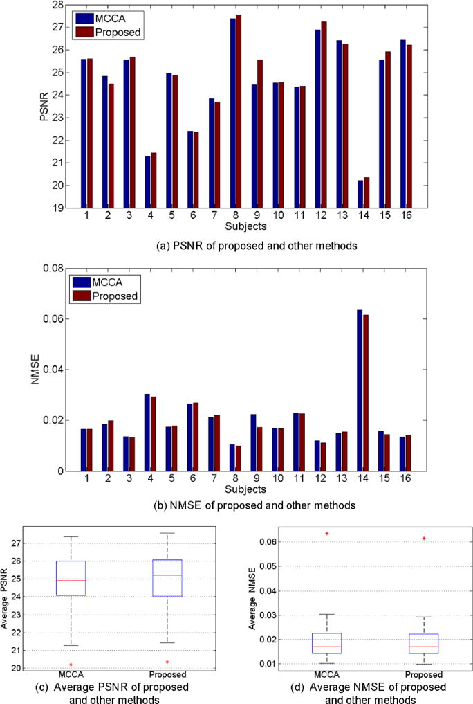
Comparisons of our proposed deep auto-context CNNs with the MCCA method. (a) and (b) show the evaluation results of PNSR and NMSE scores for all 16 subjects in the leave-one-out testing. (c) and (d) give the average results of PSNR and NMSE of all the subjects.

Importantly, our method behaves significantly better in terms of its processing time especially in testing. Table 2 compares the time costs of our method and MCCA for both training and testing. Although our method spends more time on training, the testing procedure is much faster. Concretely, it only takes 2.03 seconds to test a subject by our method, while 1,008 seconds by MCCA. The main reason is that MCCA optimizes sparse coding problems in testing, whereas our method is a completely feed-forward convolution operation without any pre-/post-processing. All the experiments are carried out on an ordinary computer with Intel Core i7 4.00GHz processor, 16 GB RAM, and an NVIDIA Geforce GTX Titan X GPU.

Table 2.

Training time and testing time of two different methods.

Method	Training Time	Testing Time
MCCA	2.9h	1008s
Proposed	4.2h	2.03s

Though our method carries out the computation from the axial plane slice by slice, the estimated results are still satisfactory in 3D view. In particular, after we complete the estimation upon all the slices, we stack them back to get the 3D image volume. A subject is shown in Fig. 9(b), where the axial, sagittal and coronal views are all available. We conclude that our estimation still appears to be isotropic, even though the CNN-based learning happens on the axial plane.

5. Conclusion

In this paper, we propose a novel deep auto-context CNN architecture for SPET image estimation using multimodality data, including both LPET and T1 images. Different from previous sparse-learning-based techniques that contain time-consuming steps such as patch representation, nonlinear mapping and reconstruction, our proposed method uses a deep neural network to map the inputs to the output directly, without any pre/post-processing beyond the optimization in the training stage. When testing a subject, our method performs a single feed-forward to get the estimation result. In this way, our method can conduct the estimation of SPET very fast. Experimental results on a real human brain image dataset demonstrate that, compared to state-of-the-art method, our method has achieved competitive estimation quality, but it is up to 500 × faster.

We have also shown that our auto-context strategy is capable of building a very deep CNN architecture to further promote the estimate quality. Meanwhile, the entire network is still trained in an end-to-end way with back-propagation. Our model can be applied to other similar applications such as mapping one modality to the other. In the future, we will investigate the acceleration of the training process to make this method more efficient.

Biographies

Lei Xiang is currently pursuing his Ph.D degree at the school of biomedical engineering, Shanghai Jiao Tong University, Shanghai, China. His research interests include medical image processing, deep learning and pattern recognition.

Yu Qiao is a Full Professor with Shenzhen Institutes of Advanced Technology Chinese Academy of Sciences, Shenzhen, China. His research interests include Computer Vision, Deep Learning, Pattern Recognition, Speech Processing, Robotics etc.

Dong Nie is currently pursuing his Ph.D degree at Department of Computer Science, University of North Carolina at Chapel Hill, America. His current research focus on Medical Image Analysis with Machine Learning.

Le An is currently an Associate Professor at School of Automation, Huazhong University of Science and Technology. His research is primarily focused on pattern recognition, computer vision, machine learning, and image processing, with applications in surveillance, biometrics, affective computing, and medical image analysis.

Qian Wang is an Associate Professor of Biomedical Engineering. He received his Ph.D. degree in Computer Science from the University of North Carolina at Chapel Hill in 2013. He has published about 40 peer-reviewed papers in the past five years, which have been cited for more than 260 times. His research focuses on medical image analysis, computer vision, machine learning, and artificial intelligence. His interest extends to large-scale populations of multi-modal, multiorgan, and multidimensional image data.

Dinggang Shen is a Professor of Radiology, Biomedical Research Imaging Center (BRIC), Computer Science, and Biomedical Engineering in University of North Carolina at Chapel Hill. Dr. Shen has published 700 articles in journals and proceedings of international conferences. Dr. Shen’s research interests include: Medical image analysis; computer vision; and pattern recognition.

References

- 1.Avril NE, Weber WA. Monitoring response to treatment in patients utilizing PET. Radiologic clinics of North America. 2005;43(1):189–204. doi: 10.1016/j.rcl.2004.09.006. [DOI] [PubMed] [Google Scholar]
- 2.Juweid ME, Stroobants S, Hoekstra OS, et al. Use of positron emission tomography for response assessment of lymphoma: consensus of the Imaging Subcommittee of International Harmonization Project in Lymphoma. Journal of Clinical Oncology. 2007;25(5):571–578. doi: 10.1200/JCO.2006.08.2305. [DOI] [PubMed] [Google Scholar]
- 3.Vansteenkiste J, Stroobants S. The role of positron emission tomography with 18F-fluoro-2-deoxy-D-glucose in respiratory oncology. European Respiratory Journal. 2001;17(4):802–820. doi: 10.1183/09031936.01.17408020. [DOI] [PubMed] [Google Scholar]
- 4.de Geus-Oei LF, van der Heijden HF, Corstens FH, et al. Predictive and prognostic value of FDG-PET in nonsmall-cell lung cancer. Cancer. 2007;110(8):1654–1664. doi: 10.1002/cncr.22979. [DOI] [PubMed] [Google Scholar]
- 5.Boellaard R. Standards for PET image acquisition and quantitative data analysis. Journal of nuclear medicine. 2009;50(Suppl 1):11S–20S. doi: 10.2967/jnumed.108.057182. [DOI] [PubMed] [Google Scholar]
- 6.Weber WA. Use of PET for monitoring cancer therapy and for predicting outcome. Journal of Nuclear Medicine. 2005;46(6):983–995. [PubMed] [Google Scholar]
- 7.Buchbender C, Heusner TA, Lauenstein TC, et al. Oncologic PET/MRI, part 1: tumors of the brain, head and neck, chest, abdomen, and pelvis. Journal of Nuclear Medicine. 2012;53(6):928–938. doi: 10.2967/jnumed.112.105338. [DOI] [PubMed] [Google Scholar]
- 8.Slovis TL. The ALARA Concept in Pediatric CT: Myth or Reality? Radiology. 2002;223(1):5–6. doi: 10.1148/radiol.2231012100. [DOI] [PubMed] [Google Scholar]
- 9.Mejia JM, Ochoa Dominguez HDJ, Vergara Villegas OO, et al. Noise reduction in small-animal PET images using a multiresolution transform. Medical Imaging, IEEE Transactions on. 2014;33(10):2010–2019. doi: 10.1109/TMI.2014.2329702. [DOI] [PubMed] [Google Scholar]
- 10.Le Pogam A, Hanzouli H, Hatt M, et al. Denoising of PET images by combining wavelets and curvelets for improved preservation of resolution and quantitation. Medical image analysis. 2013;17(8):877–891. doi: 10.1016/j.media.2013.05.005. [DOI] [PubMed] [Google Scholar]
- 11.Bagci U, Mollura DJ. Medical Image Computing and Computer-Assisted Intervention–MICCAI 2013. Springer; 2013. Denoising PET images using singular value thresholding and stein’s unbiased risk estimate; pp. 115–122. [DOI] [PMC free article] [PubMed] [Google Scholar]
- 12.Gervaise A, Osemont B, Lecocq S, et al. CT image quality improvement using adaptive iterative dose reduction with wide-volume acquisition on 320-detector CT. European radiology. 2012;22(2):295–301. doi: 10.1007/s00330-011-2271-7. [DOI] [PubMed] [Google Scholar]
- 13.Zhang W, Li R, Deng H, et al. Deep convolutional neural networks for multimodality isointense infant brain image segmentation. NeuroImage. 2015;108:214–224. doi: 10.1016/j.neuroimage.2014.12.061. [DOI] [PMC free article] [PubMed] [Google Scholar]
- 14.Wang Y, Zhang P, An L, et al. Predicting standard-dose PET image from low-dose PET and multimodal MR images using mapping-based sparse representation. Physics in medicine and biology. 2016;61(2):791. doi: 10.1088/0031-9155/61/2/791. [DOI] [PubMed] [Google Scholar]
- 15.Turkheimer FE, Boussion N, Anderson AN, et al. PET image denoising using a synergistic multiresolution analysis of structural (MRI/CT) and functional datasets. Journal of Nuclear Medicine. 2008;49(4):657–666. doi: 10.2967/jnumed.107.041871. [DOI] [PubMed] [Google Scholar]
- 16.Nguyen VG, Lee SJ. Incorporating anatomical side information into PET reconstruction using nonlocal regularization. Image Processing, IEEE Transactions on. 2013;22(10):3961–3973. doi: 10.1109/TIP.2013.2265881. [DOI] [PubMed] [Google Scholar]
- 17.Huynh T, Gao Y, Kang J, et al. Estimating ct image from mri data using structured random forest and auto-context model. IEEE transactions on medical imaging. 2016;35(1):174–183. doi: 10.1109/TMI.2015.2461533. [DOI] [PMC free article] [PubMed] [Google Scholar]
- 18.Tu Z, Bai X. Auto-context and its application to high-level vision tasks and 3d brain image segmentation. Pattern Analysis and Machine Intelligence, IEEE Transactions on. 2010;32(10):1744–1757. doi: 10.1109/TPAMI.2009.186. [DOI] [PubMed] [Google Scholar]
- 19.Wang Y, Ma G, An L, et al. Semi-Supervised Tripled Dictionary Learning for Standard-dose PET Image Prediction using Low-dose PET and Multimodal MRI. 2016 doi: 10.1109/TBME.2016.2564440. [DOI] [PMC free article] [PubMed] [Google Scholar]
- 20.An L, Zhang P, Adeli E, et al. Multi-Level Canonical Correlation Analysis for Standard-Dose PET Image Estimation. IEEE Transactions on Image Processing. 2016;25(7):3303–3315. doi: 10.1109/TIP.2016.2567072. [DOI] [PMC free article] [PubMed] [Google Scholar]
- 21.LeCun Y, Boser B, Denker JS, et al. Backpropagation applied to handwritten zip code recognition. Neural computation. 1989;1(4):541–551. [Google Scholar]
- 22.Simonyan K, Zisserman A. Very deep convolutional networks for large-scale image recognition. arXiv preprint arXiv:1409.1556. 2014 [Google Scholar]
- 23.Krizhevsky A, Sutskever I, Hinton GE. Imagenet classification with deep convolutional neural networks. :1097–1105. [Google Scholar]
- 24.Sun Y, Wang X, Tang X. Deep convolutional network cascade for facial point detection. :3476–3483. [Google Scholar]
- 25.Taigman Y, Yang M, Ranzato MA, et al. Deepface: Closing the gap to human-level performance in face verification. :1701–1708. [Google Scholar]
- 26.Sun Y, Wang X, Tang X. Deep learning face representation from predicting 10,000 classes. :1891–1898. [Google Scholar]
- 27.Long J, Shelhamer E, Darrell T. Fully convolutional networks for semantic segmentation. :3431–3440. doi: 10.1109/TPAMI.2016.2572683. [DOI] [PubMed] [Google Scholar]
- 28.Chen LC, Papandreou G, Kokkinos I, et al. Semantic image segmentation with deep convolutional nets and fully connected crfs. arXiv preprint arXiv:1412.7062. 2014 doi: 10.1109/TPAMI.2017.2699184. [DOI] [PubMed] [Google Scholar]
- 29.Hong S, You T, Kwak S, et al. Online tracking by learning discriminative saliency map with convolutional neural network. arXiv preprint arXiv:1502.06796. 2015 [Google Scholar]
- 30.Li H, Li Y, Porikli F. DeepTrack: Learning Discriminative Feature Representations by Convolutional Neural Networks for Visual Tracking. :3. [Google Scholar]
- 31.Ma C, Huang JB, Yang X, et al. Hierarchical Convolutional Features for Visual Tracking. :3074–3082. doi: 10.1109/TPAMI.2018.2865311. [DOI] [PubMed] [Google Scholar]
- 32.Cruz-Roa AA, Ovalle JEA, Madabhushi A, et al. A deep learning architecture for image representation, visual interpretability and automated basal-cell carcinoma cancer detection. :403–410. doi: 10.1007/978-3-642-40763-5_50. [DOI] [PubMed] [Google Scholar]
- 33.Xu J, Xiang L, Liu Q, et al. Stacked sparse autoencoder (SSAE) for nuclei detection on breast cancer histopathology images. IEEE transactions on medical imaging. 2016;35(1):119–130. doi: 10.1109/TMI.2015.2458702. [DOI] [PMC free article] [PubMed] [Google Scholar]
- 34.Zhu Q, Du B, Turkbey B, et al. Deeply-Supervised CNN for Prostate Segmentation. arXiv preprint arXiv:1703.07523. 2017 [Google Scholar]
- 35.Liao S, Gao Y, Oto A, et al. Representation learning: a unified deep learning framework for automatic prostate MR segmentation. :254–261. doi: 10.1007/978-3-642-40763-5_32. [DOI] [PMC free article] [PubMed] [Google Scholar]
- 36.Nair V, Hinton GE. Rectified linear units improve restricted boltzmann machines. :807–814. [Google Scholar]
- 37.Srivastava N, Hinton G, Krizhevsky A, et al. Dropout: A simple way to prevent neural networks from overfitting. The Journal of Machine Learning Research. 2014;15(1):1929–1958. [Google Scholar]
- 38.Deng J, Dong W, Socher R, et al. Imagenet: A large-scale hierarchical image database. :248–255. [Google Scholar]
- 39.Ioffe S, Szegedy C. Batch normalization: Accelerating deep network training by reducing internal covariate shift. arXiv preprint arXiv:1502.03167. 2015 [Google Scholar]
- 40.Li R, Zhang W, Suk HI, et al. Medical Image Computing and Computer-Assisted Intervention–MICCAI. Springer; 2014. Deep learning based imaging data completion for improved brain disease diagnosis; pp. 305–312. 2014. [DOI] [PMC free article] [PubMed] [Google Scholar]
- 41.Dong C, Loy CC, He K, et al. Image super-resolution using deep convolutional networks. IEEE transactions on pattern analysis and machine intelligence. 2016;38(2):295–307. doi: 10.1109/TPAMI.2015.2439281. [DOI] [PubMed] [Google Scholar]
- 42.Dong C, Loy CC, He K, et al. Image super-resolution using deep convolutional networks. 2015 doi: 10.1109/TPAMI.2015.2439281. [DOI] [PubMed] [Google Scholar]
- 43.LeCun Y, Bottou L, Bengio Y, et al. Gradient-based learning applied to document recognition. Proceedings of the IEEE. 1998;86(11):2278–2324. [Google Scholar]
- 44.Lee CY, Xie S, Gallagher P, et al. Deeply-supervised nets. arXiv preprint arXiv:1409.5185. 2014 [Google Scholar]
- 45.Chen H, Qi XJ, Cheng JZ, et al. Deep contextual networks for neuronal structure segmentation [Google Scholar]
- 46.Smith SM, Jenkinson M, Woolrich MW, et al. Advances in functional and structural MR image analysis and implementation as FSL. Neuroimage. 2004;23:S208–S219. doi: 10.1016/j.neuroimage.2004.07.051. [DOI] [PubMed] [Google Scholar]
- 47.Shi F, Wang L, Dai Y, et al. LABEL: pediatric brain extraction using learning-based meta-algorithm. Neuroimage. 2012;62(3):1975–1986. doi: 10.1016/j.neuroimage.2012.05.042. [DOI] [PMC free article] [PubMed] [Google Scholar]
- 48.Fischer B, Modersitzki J. Biomedical Image Registration. Springer; 2003. FLIRT: a flexible image registration toolbox; pp. 261–270. [Google Scholar]
- 49.Jia Y, Shelhamer E, Donahue J, et al. Caffe: Convolutional architecture for fast feature embedding. :675–678. [Google Scholar]
- 50.Jain V, Seung S. Natural image denoising with convolutional networks. :769–776. [Google Scholar]