. 2017 Dec 5;6:e22901. doi: 10.7554/eLife.22901

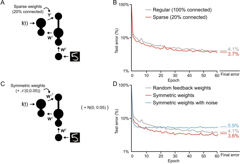
Figure 8. Conditions on feedback synapses for effective learning.

(A) Diagram of a one hidden layer network trained in B, with 80% of feedback weights set to zero. The remaining feedback weights Y were multiplied by five in order to maintain a similar overall magnitude of feedback signals. (B) Plot of test error across 60 epochs for our standard one hidden layer network (gray) and a network with sparse feedback weights (red). Sparse feedback weights resulted in improved learning performance compared to fully connected feedback weights. Right: Spreads (min – max) of the results of repeated weight tests (n=20) after 60 epochs for each of the networks. Percentages indicate mean final test errors for each network (two-tailed t-test, regular vs. sparse: t38=16.43, p=7.4×10¹⁹). (C) Diagram of a one hidden layer network trained in D, with feedback weights that are symmetric to feedforward weights W1, and symmetric but with added noise. Noise added to feedback weights is drawn from a normal distribution with variance σ=0.05. (D) Plot of test error across 60 epochs of our standard one hidden layer network (gray), a network with symmetric weights (red), and a network with symmetric weights with added noise (blue). Symmetric weights result in improved learning performance compared to random feedback weights, but adding noise to symmetric weights results in impaired learning. Right: Spreads (min – max) of the results of repeated weight tests (n=20) after 60 epochs for each of the networks. Percentages indicate means (two-tailed t-test, random vs. symmetric: t38=18.46, p=4.3×10²⁰; random vs. symmetric with noise: t38=-71.54, p=1.2×1041; symmetric vs. symmetric with noise: t38=-80.35, p=1.5×1043, Bonferroni correction for multiple comparisons).

Figure 8—source data 1. Fig_8B_errors.csv.
This data file contains the test error (measured on 10,000 MNIST images not used for training) across 60 epochs of training, for our standard one hidden layer network (Regular) and a network with sparse feedback weights. Fig_8B_final_errors.csv. This data file contains the results of repeated weight tests (n=20) after 60 epochs for each of the two networks described above. Fig_8D_errors.csv. This data file contains the test error (measured on 10,000 MNIST images not used for training) across 60 epochs of training, for our standard one hidden layer network (Regular), a network with symmetric weights, and a network with symmetric weights with added noise. Fig_8D_final_errors.csv. This data file contains the results of repeated weight tests (n=20) after 60 epochs for each of the three networks described above. Fig_8S1_errors.csv. This data file contains the test error (measured on 10,000 MNIST images not used for training) across 20 epochs of training, for a one hidden layer network with regular feedback weights, sparse feedback weights that were amplified, and sparse feedback weights that were not amplified. Fig_8S1_final_errors.csv. This data file contains the results of repeated weight tests (n=20) after 20 epochs for each of the three networks described above.
DOI: 10.7554/eLife.22901.017

Figure 8.

Figure 8—figure supplement 1. Importance of weight magnitudes for learning with sparse weights.
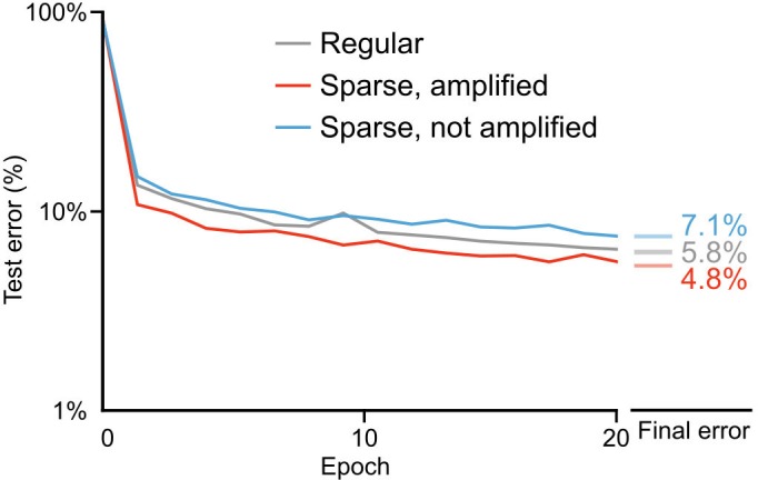
Figure 8—figure supplement 1.

Plot of test error across 20 epochs of training on MNIST of a one hidden layer network, with regular feedback weights (gray), sparse feedback weights that were amplified (red), and sparse feedback weights that were not amplified (blue). The network with amplified sparse feedback weights is the same as in Figure 8A and B, where feedback weights were multiplied by a factor of 5. While sparse feedback weights that were amplified led to improved training performance, sparse weights without amplification impaired the network’s learning ability. Right: Spreads (min – max) of the results of repeated weight tests (n=20) after 20 epochs for each of the networks. Percentages indicate means (two-tailed t-test, regular vs. sparse, amplified: t38=44.96, p=4.4×1034; regular vs. sparse, not amplified: t38=-51.30, p=3.2×1036; sparse, amplified vs. sparse, not amplified: t38=-100.73, p=2.8×1047, Bonferroni correction for multiple comparisons).