Hybrid deep learning on single wide-field optical coherence tomography scans accurately classifies glaucoma suspects

Abstract

Purpose

Existing summary statistics based upon optical coherence tomography (OCT) scans and/or visual fields (VF) are suboptimal for distinguishing between healthy and glaucomatous eyes in the clinic. This study evaluates the extent to which a hybrid deep learning method (HDLM), combined with a single wide-field OCT protocol, can distinguish eyes previously classified as either healthy suspects or mild glaucoma.

Patients and Methods

102 eyes from 102 patients, with or suspected open-angle glaucoma, had previously been classified by two glaucoma experts as either glaucomatous (57 eyes) or healthy/suspects (45 eyes). The HDLM had access only to information from a single, wide-field (9×12mm) swept-source OCT scan per patient. Convolutional neural networks were used to extract rich features from maps derived from these scans. Random forest classifier was used to train a model based on these features to predict the existence of glaucomatous damage. The algorithm was compared against traditional OCT and VF metrics.

Results

The accuracy of the HDLM ranged from 63.7% to 93.1% depending upon the input map. The RNFL probability map had the best accuracy (93.1%), with 4 false positives, and 3 false negatives. In comparison, the accuracy of the OCT and 24-2 and 10-2 VF metrics ranged from 66.7% to 87.3%. The OCT quadrants analysis had the best accuracy (87.3%) of the metrics, with 4 FP and 9 FN.

Conclusion

The HDLM protocol outperforms standard OCT and VF clinical metrics in distinguishing healthy suspect eyes from eyes with early glaucoma. It should be possible to further improve this algorithm and with improvement it might be useful for screening

Introduction

The detection of glaucoma, especially in the early stages of the disease, can present a challenge for clinicians who care for glaucoma patients. We recently argued that a single wide-field optical coherence tomography (OCT) scan has the information needed to distinguish healthy suspect eyes from eyes with early glaucoma.¹ In particular, two glaucoma specialists placed 102 eyes into two groups (glaucoma or probably glaucoma versus healthy or probably healthy) based upon information from the patients’ charts, 24-2 and 10-2 visual fields (VFs), and OCT scans. Using only a single-page report that summarized the results from a single wide-field OCT scan, the senior author (DCH) correctly identified 100 of these eyes for an accuracy of 98%. This result was surprising because many of these eyes were particularly challenging. Specifically, they all had 24-2 VFs with mean deviations (MD) better than -6dB and an abnormal and/or anomalous disc referred to a tertiary care glaucoma specialist.

However, there are at least two reasons for tempering the enthusiasm for this finding. First, it remains to be seen if others can do as well as the OCT specialist in that study, who had many years of experience with glaucomatous damage seen on OCT scans. Further, even if we assume others can be trained to do as well, the amount of training needed remains to be determined.

In this study, we explore the extent to which these two limitations can be overcome with a machine learning method. In particular, we evaluate the extent to which a computer vision based hybrid deep learning method (HDLM), using the single wide-field OCT protocol, can distinguish healthy from abnormal eyes in the same group of 102 eyes previously classified as either healthy suspects or mild glaucoma.

Methods

Patients

102 eyes from 102 patients with a diagnosis of glaucoma or glaucoma suspect, gonioscopically open angles, a 24-2 VF MD better than −6 dB, and a spherical refractive error between ±6° were included. In addition to the 24-2 VF, all patients were also tested with the 10-2 test pattern (Humphrey Field Analyzer; Carl Zeiss Meditec, Inc, Dublin, CA) within <6 months of the 24-2 test. Written, informed consent was obtained from all participants. Procedures followed the tenets of the Declaration of Helsinki, and the protocol was approved by the institutional review boards of Columbia University and the New York Eye and Ear Infirmary of Mount Sinai.

The 102 eyes were part of a previous study,¹ which started with 130 eyes. In that study, two glaucoma specialists judged each eye as healthy (H); probably healthy (PH); forced-choice healthy (FC-H); glaucomatous (G); probably G (PG); forced-choice G (FC-G) based upon 24-2 and 10-2 VFs, fundus photos, patient chart information, and a single-page OCT report,² which included an OCT specialist’s interpretation as indicated in ref 1. The forced-choice categories were used if the specialists were not sure, but had to guess. For a reference standard in this study, the 57 eyes judged G or PG by both glaucoma specialists were considered “glaucomatous”, and the 45 eyes judged H or PH by both were considered “healthy”. Note: 28 of the original 130 eyes in ref. 1 were not included in that study or this one. Of these, the two glaucoma specialists did not agree on 23 eyes, while the other 5 had optic neuropathies.¹

Optical Coherence Tomography

All patients were scanned using a swept-source OCT (DRI OCT-1 Atlantis, Topcon, Inc, Tokyo, Japan) and a wide-field cube scan protocol (12 × 9 mm, 256 horizontal B-scans with 512 A scans each), which included the macular and disc regions. The thicknesses of the retinal nerve fiber layer (RNFL) and retinal ganglion cell plus inner plexiform layer (RGC+) were determined by using the OCT instrument’s software (v9.30beta). Figure 1 shows the region of the retina covered (A), along with a representative b-scan (B) with the RGC+ and RNFL borders indicated. Based upon the software’s segmentation of these borders thickness maps were created as standard 3-color channel images for both RGC+ (C) and RNFL (D).

Figure 1.

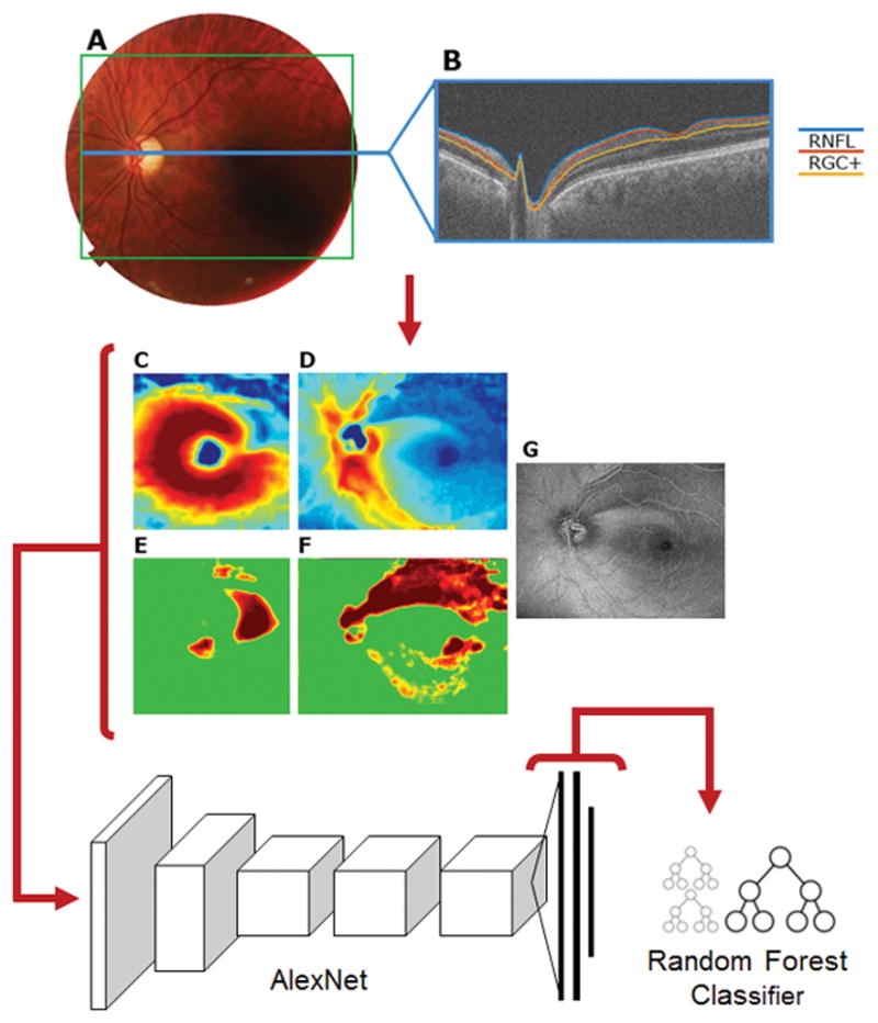
(A) A fundus photo of a scanned eye with a green box outlining the area scanned by OCT and a blue line corresponding to one B-scan (B). An example of an RGC+ thickness map (C) and an RNFL thickness map (D), as well as their corresponding probability maps (E and F). (G) a 50 μm en face projection image. These images are fed into AlexNet. 4096 features are extracted in the output and used as input to train a random forest classifier.

Based upon these thickness data and machine normals, we also produced probability maps rendered in 3-color channel images. In the case of the RNFL probability map (Fig. 1F), it included the entire scan region, while in the case of the RGC+ probability map (Fig. 1E), it was restricted to a 6x6mm region centered on the fovea. Further, en face projection images (also in 3-color channel) were generated for each patient by averaging pixels vertically in a 50 μm slab beneath the inner limiting membrane (Fig. 1G) as described in a previous study. ³

Convolutional Neural Networks

Unlike standard deep neural networks which update the weights of nodes (or “neurons”) through learning, convolutional neural networks (CNN) learn kernels, or filters, to convolve across inputs in order to extract features from 3-D tensors, specifically images (width × height × three color channels) and pass them to the next layer. Images fed-forward through multiple convolutional layers and are reduced to abstract features. Thus, nodes in the first convolutional layer are tuned to basic features of an image, such as edge gradients in various directions or color blobs of different hue combinations. The second convolutional layer takes the weights of these basic features and further convolves them into more complex representations. Depending on the design of the network, other layers in the network exist between the convolutional layers: A rectified linear units (ReLU) layer, which applies a fixed activation function and a pooling layer, which down-samples the spatial dimensions of data passing through the network to reduce number of parameters. Finally, towards the end of the model, there are fully-connected layers, which together, resemble traditional neural networks and perform the bulk of the classification computing on information coming from the convolutional layers. The organization and placement of these different layers can vary among different CNN models.

Model Design

In this study we argue for the use of a pre-trained CNN model for feature extraction and a random forest model for classification. The weights of the nodes (what we refer to as features) in the fully connected layers of the neural network are used as input for the random forest.

In particular, feature extraction was performed with the Caffe⁴ deep learning framework on a high performance compute cluster running CentOS. Processing was done on two GPUs (Titan X, NVIDIA Inc., Santa Clara, CA) connected in parallel under a subnode (Xeon E7, Intel Inc., Santa Clara, CA). The pre-trained model used was AlexNet⁵ due to its well-studied performance and simplicity of structure. Further, AlexNet was the winning model of the ILSVRC2012 classification task, a community benchmark for computer vision algorithms.⁶

For each subject, 6 images in lossless png format were used as input for the CNN: (1) RGC+ thickness map (Fig. 1C); (2) RNFL thickness map (Fig. 1D), (3) RGC+ probability map (Fig. 1E); (4) RFNL probability map (Fig. 1F), (5) en face projection (Fig. 1G). A sixth image, a combination of (2, 3, and 4) was also evaluated. This “combined” image was constructed by replacing the red-channel of the image with RNFL probability values, the green-channel with RGC+ probability values, and the blue-channel with normalized RNFL thickness values. Because AlexNet was trained on natural images, all color channels are assumed to be considered equally by the network. The ordering of maps in the color channels may minimally affect performance. A vertically flipped copy of each image type was also fed into the CNN in order to increase the training efficacy for the learning step. Note that this step is based around the notion of vertical invariancy and not the assumption that the data is symmetrical about the x-axis - such data augmentations for image classification tasks have been shown to significantly improve prediction accuracy previously.⁷

The final three layers of AlexNet (fc6, fc7, and fc8) are one-dimensional fully connected layers. Layers fc6 and fc7 have 4096 features each and fc8, which normally serves as an output classifier, has 1000 features, one for each of the 1000 classes in the ImageNet database⁸ that AlexNet was trained on. In our case, instead of using the probability-based class predictions in the final output layer, we used the associated weights to evaluate if they contain information about glaucomatous damage inferred from the OCT-based images. Finally, the three arrays of features for each of the 6 types of images were used for training and testing.

Random Forest Classifier

To classify patients into “healthy” and “glaucomatous” we trained a random forest (RF) classifier, based on the feature vector from the CNN. The model was evaluated for each of the 6 image types by conducting leave-one-out cross-validation. Random forests^9,10 are ensemble classifiers based on decision trees that are grown by bootstrapping the training dataset and randomly selecting feature subsets at each split node. Each tree makes a prediction for an input sample based on its construction during training and the decision with the most votes (trees) is the predicted classification label. In our case, the labels were “healthy” and “glaucomatous.” Our final model consisted of 200 trees, which were trained in parallel on a compute cluster. Because there can be variance in the results of random forest, this method was repeated 50 times.

Evaluation of Performance

The statistical analysis was conducted in R¹¹ (version 3.1.1). Modifications were made in both the CNN and RF code base. For the CNN, a comparison of the three fully connected layers and a combination of all three was done on each image type to assess the layer with the best performing features. In each case, layer fc6 yielded the best area under the curve of receiver operating characteristic curve (AROC) based on the probability of trees which voted “Glaucomatous” for each subject (see Table 1 for the average AROC across 50 trials). From here on, we will only discuss results based upon this layer.

Table 1.

Average AROC values and 95% confidence intervals (CI) across 50 trials for each fully connected layer for each image type.

Comparing classification performance of fully connected layers
	fc6		fc7		fc8		fc6+fc7+fc8
	Mean	95% CI	Mean	95% CI	Mean	95% CI	Mean	95% CI
RNFL Thickness	.973	.972,.974	.962	.961,.964	.956	.954,.957	.973	.972,.974
RGC+ Thickness	.938	.937,.940	.936	.934,.937	.932	.931,.933	.935	.934,.936
RNFL Probability	.961	.960,.962	.957	.956,.958	.958	.957,.959	.979	.976,.980
RGC+ Probability	.920	.920,.921	.920	.920,.920	.913	.911,.914	.950	.949,.951
en face Projection	.742	.737,.747	.697	.692,.701	.688	.683,.694	.758	.754,.761
Combined	.945	.944,.947	.902	.900,.903	.885	.884,.886	.919	.917,.920

Because of the stochastic properties of RFs, the structure of the trees is different with each training run. Thus, the RF model was trained and tested 50 times, and the false-positive (FP) and false-negative (FN) of each iteration were averaged to estimate the generalization performance.

Choosing an optimal number of trees in a forest lowers computation time and avoids over and under-fitting on the model. Figure 2 shows the convergence of the out-of-bag error (i.e., a generalization of error created within the training set) as the forest grows in one iteration. The error rate converge around 100 trees. Finally, the number of correct and incorrect predictions were evaluated for a FP / FN analysis.

Figure 2.

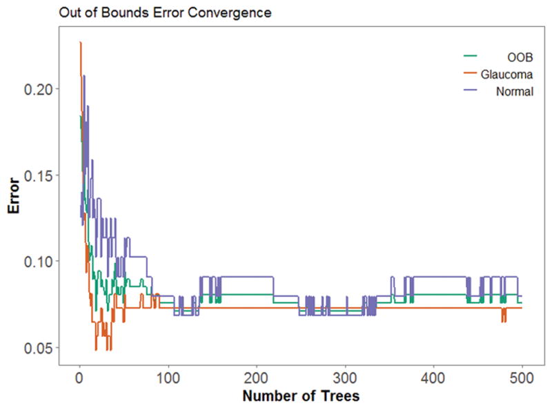
As the number of trees increases, error decreases and converges. Out-of-bounds error (red) represents the average misclassification of glaucomatous (blue) and normal (green) images.

OCT and VF Metrics

To benchmark the performance of the HDLM, conventional clinical metrics based upon OCT scans of the disc and 24-2 and 10-2 VFs were obtained.

OCT

Based upon the wide-field scan, the instrument’s software (9.30beta (Atlantis) and v1.16beta (IMAGEnet6), Topcon Inc, Tokyo, Japan) obtained the RNFL thickness along a 3.4 mm diameter circle. From these circumpapillary (cp) RNFL thickness data, the software calculated the 3 most commonly used OCT metrics: total cpRNFL thickness (T); thickness within each of the 4 quadrants around the disc (Q); and thickness within each of the 12 clock hours around the disc (CH). For Q, an eye with one or more quadrants falling below the 5% confidence limit (CI) was considered abnormal. For CH, an eye was considered abnormal if one of more clock hours fell below the 1% CI or two or more contiguous clock hours fell below the 5% CI. For T, an eye was considered abnormal if the total cpRNFL thickness fell below 96μm, chosen for best accuracy.

24-2 VF

The following metrics were used: mean deviation (MD) with P ≤5%; pattern standard deviation (PSD) with P≤5%; a glaucoma hemifield test (GHT) outside normal limits; and a cluster criteria (CC) of 3 neighboring points at 5, 5, and 1% or 5, 2, and 2% probability or worse within a hemifield on total deviation (TD) or pattern deviation (PD) plots, with only one point allowed on the edge of the 24-2 VF test pattern. In addition, the criteria used in the OHTS, an abnormal GHT or PSD, was also considered.

10-2 VF

The following metrics were used: mean deviation (MD) with P ≤5%; PSD with P ≤5%; and a cluster criteria (CC) of 3 neighboring points at 5, 5, and 1% or 5, 2, and 2% probability or worse within a hemifield on TD or PD plots.

The accuracy of the best performing HDLM was compared to each conventional clinical metric using a one-sample test with reported confidence intervals.

Results

Each trial of the RF model produced slightly different result because decision trees grow based upon random bootstrapping of training data. An assessment of the effects on accuracy by the stochastic properties of RF is shown in Figure 3. The small symbols are the results from individual runs for 50 trials of each of the six image types. The boundaries of the box show the 25% and 75% quartiles, and the whiskers show the maximum and minimum values. There was low variability in classification error. RNFL probability yielded the highest average accuracy and the least variability, 92.4 ± 0.57%, the en face projections yielded the lowest average accuracy and the greatest variability, 65.7 ± 1.53%. Figure 4 shows the ROC of one randomly chosen trial.

Figure 3.

Error distribution across trials is shown for each image. The 50 trials for each image are shown as the small data points near the boxplots. The width of the box is the 25% to 75% quartile range. The whiskers represent minimum and maximum values.

Figure 4.

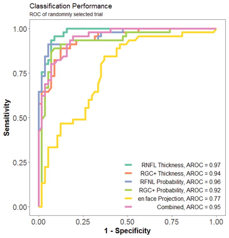
A receiver operating curve (ROC) for one randomly selected trial.

Table 2 shows the results of the FP/FN analysis as modal values across trials. The RNFL probability had the best modal accuracy, 93.1% and average accuracy, 92.6%; it missed 7 eyes with 3 FN and 4 FP.

Table 2.

False positive/false negative rates, average area under receiver operator characteristic (AROC), modal accuracy, and average accuracy for each type of image.

Average Accuracy and FP/FN Rate of Model
Paradigm	False Negatives N=57	False Positives N=45	Average AROC N=102	Modal Accuracy N=102	Average Accuracy N=102
RNFL Thickness	4	7	.973	89.2%	89.7±1.02%
RGC+ Thickness	7	8	.938	85.3%	85.5±1.01%
RNFL Probability	3	4	.961	93.1%	92.6±0.57%
RGC+ Probability	5	7	.920	88.2%	88.6±0.76%
en face Projection	12	25	.742	63.7%	63.6±1.53%
Combined	8	6	.945	86.3%	86.2±1.06%

A comparison to conventional OCT and VF metrics

The RNFL probability did better than any of the typically used metrics derived from OCT disc scans (Table 3), 24-2 (Table 4) or 10-2 (Table 5) VFs. For the OCT metrics, the quadrants (Q) had the best accuracy, 87.3%. However, it missed 13 eyes (9 FN and 4 FP), nearly twice as many as the HDLM with RNFL probability images. The VF metrics performed more poorly than the OCT (Tables 4 and 5). The best metric (PSD or GHT) for the 24-2 VFs had an accuracy of 80.4% with a total of 20 misses. The MD, PSD or cluster criteria of the 10-2 VFs had a similar accuracy, 80.4%. A significant increase in performance was seen versus all metrics when using RNFL Probabbilty HDLM (p < .001).

Table 3.

False positive/false negative rates and accuracy of typical clinical OCT metrics. Further, a measure of improvement when using best HDLM method (RNFL Probability) with associated confidence intervals.

Performance of Clinical OCT Metrics
OCT Metrics	False Negatives N=57	False Positives N=45	Accuracy N=102	Difference from Best HDLM	95% CI
Q	9	4	87.3	3.68	3.52, 3.85
CH	12	2	86.3	4.68	4.52, 4.85
T (<96.0 um)	10	5	85.3	5.68	5.52, 5.85
Any 1 of 3	8	8	84.3	6.68	6.52, 6.85

(Q = thickness within each of the 4 quadrants around the disc, CH = thickness within each of the 12 clock hours around the disc, T = total cpRNFL thickness).

Table 4.

False positive/false negative rates and accuracy of typical clinical 24-2 visual field (VF) metrics. Further, a measure of improvement when using best HDLM method (RNFL Probability) with associated confidence intervals.

Performance of Clinical 24-2 VF Metrics
24-2 VF Metrics	False Negatives N=57	False Positives N=45	Accuracy N=102	Difference from Best HDLM	95% CI
MD	23	7	70.5%	24.28	24.12, 24.45
PSD	14	6	80.3%	11.58	11.42, 11.75
GHT	19	2	79.4%	12.58	12.42, 12.75
CC	9	17	74.5%	16.48	16.32, 16.65
PSD or GHT	13	7	80.4%	10.58	10.42, 10.75
Any 1 of 4	6	20	74.5%	16.48	16.32, 16.65

(MD = mean deviation, PSD = pattern standard deviation, GHT = glaucoma hemifield test, CC = 5-5-1 cluster criteria).

Table 5.

False positive/false negative rates and accuracy of typical clinical 12-2 visual field (VF) metrics. Further, a measure of improvement when using best HDLM method (RNFL Probability) with associated confidence intervals.

Performance of Clinical 10-2 VF Metrics
10-2 VF Metrics	False Negatives N=57	False Positives N=45	Accuracy N=102	Difference from Best HDLM	95% CI
MD	27	7	66.7%	24.28	24.12, 24.45
PSD	21	3	76.5%	14.48	14.32, 14.65
CC	9	12	79.4%	11.58	11.42, 11.75
1 of 3	8	12	80.4%	10.58	10.42, 10.75

(MD = mean deviation, PSD = pattern standard deviation, GHT = glaucoma hemifield test, CC = 5-5-1 cluster criteria).

An analysis of FP and FN

To better understand why the HDLM with the RNFL probability map missed 8 eyes, the single page reports available to the OCT specialist were analyzed. Of the 4 healthy eyes misclassified as abnormal by the HDLM, all had what appeared to be arcuate defects on the RNFL probability plot. Figure 5A shows the report available to the OCT specialist for one of these eyes. The specialist rated this eye as “healthy” and was not misled by the apparent arcuate defect (black arrow) on the RNFL probability map (panel 3), which is shown in VF view. That is, the region indicated by the black arrow in panel 3 is in the superior disc in panel 2. The specialist attributed this abnormal region in the RNFL probability map to the placement of the major superior blood vessels (white arrow in Figure 5A, panel 1). The vertical red line on the peripapillary RNFL thickness plot (panel 2) represents the average location of the major blood vessels from a group of healthy individuals.¹² In this case, the superior temporal blood vessels are situated more temporal than the average location (red arrow and red vertical line in panel 2). Because the thickest portion of the superior arcuate bundle tends to follow the major superior temporal blood vessels, the peak of the RNFL thickness plot is shifted. Thus, the RNFL thickness appears abnormally thin, and falls in the abnormal region (black arrow) on the RNFL probability plot (panel 3). The OCT specialist recognized this and classified this eye as “healthy”. Similar RNFL defects are seen in the 3 other misclassified normal patients (Figure 5B–D).

Figure 5.

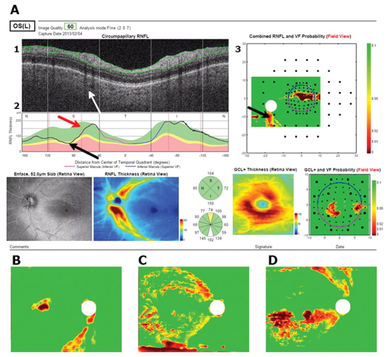
(A) A report for a false positive available to the OCT specialist. Black arrows point towards the location of the defect, red arrow points to average blood vessel location, white arrow points to location of blood vessels in example. (B – D) show RNFL probability maps of 3 other imilar examples.

Of the 3 abnormal eyes misclassified as normal by the HDLM, 2 had clear macular damage as seen on RGC+ thickness and probability plots. Figure 6A shows the RNFL probability map for one of these eyes. The HDLM with the RNFL probability map classified this eye as healthy, even though there were signs of abnormal RNFL thickness on the RNFL probability plot (black arrows). However, the report specialist could clearly see that there was damage to the macula on the RGC+ plots (black arrows in Figure 6B). The third eye showed an arcuate defect in the superior VF/inferior retina on the RNFL probability and thickness plots. Although the changes on this map were subtle, the specialist was able to confirm them by examining the en-face and RNFL thickness images, where the red arrow shows the arcuate defect (Figure 6C).

Figure 6.

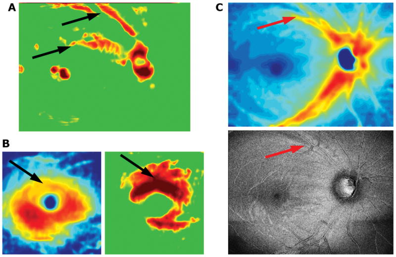
Portions of a report for an example of a false negative. Subtle defects can be seen on the RNFL (A,B) and RGC+ (C,D) thickness (B,C) and probability (A,D) maps, as well as the en face projection image (E). The red and black arrows point to abnormal regions.

Discussion

We tested the hypothesis that a HDLM, using the single wide-field OCT protocol, can distinguish healthy from abnormal eyes in a group of 102 eyes previously classified by specialists. When using the RNFL probability map, the HDLM had an average accuracy of 93.3%; it misclassified 7 eyes. In comparison, the best OCT metric missed 13 eyes and the best 24-2 and 10-2 VF metrics missed 20 eyes.

While the HDLM did well, it missed 5 more eyes than did the OCT specialist in our previous study. In that study, the specialist had available only a one-page report based upon only the same single wide-field ssOCT scan. An analysis of the 7 misclassified eyes suggests ways to improve the HDLM. In particular, it might be possible to avoid FP due to blood vessel locations if our group of healthy controls was larger and the information about blood vessels included in the HDLM. When training a network, specific neurons can learn to tune to blood vessel positions as a parameter, creating a feature which includes the information during learning. This is one of the benefits of using a model trained for the task at hand, rather than the pre-trained model used here.

Similarly, avoiding FN due to local damage restricted to the macula, which is very easy to spot on the RGC+ maps, but easy to miss on the RNFL plots (Fig. 5A), is feasible by creating a custom CNN structure to take in multiple inputs in parallel. Combining RGC+ and RNFL probability images did not yield superior results to the RNFL probability alone when using the pre-trained model. However, when assessing RGC+ on the combined fc6+fc7+fc8 feature vectors, performance based on AROC was comparable to RNFL probability on fc6. This means the CNN is sensitive to the empirical information in RGC+ images. Given a novel method to combine RNFL and RGC+ information, it is feasible to increase classification performance.

Note that the CNN learns to differentiate regions of RNFL thinning (depicted in red in probability maps) from other regions of red due to individual variation, segmentation errors, or noise. Because noise is scattered throughout all images, and damage in arcuate regions only exists in glaucomatous eyes, the RF learns to differentiate between features from the CNN that represent those two cases. This is a benefit from traditional image processing methods which require a priori mathematical representation of damage in probabilities, clusters, shapes, or intensities, before being able to detect it. Often, when using these techniques, it can be hard to differentiate noise from significant data.

The approach here is substantially different from other studies that have used machine learning or supervised learning with OCT data. Several studies have employed progression of patterns¹³ and unsupervised Gaussian mixture-models^14,15 on VF data. OCT has not been utilized to its full extent when training model machine learning based on OCT information. For example, a study which used Bayesian machine learning classifiers trained with combined structural (OCT) and functional (VF) data performed with an AROC of 0.869. OCT alone, however, performed worse with an AROC of 0.817.¹⁶ It is important to note that in the methodology, the high resolution and data rich OCT was subsampled into 32 discrete measurements of thickness, which may hinder the performance of structure-only classifiers. Reductions in data complexity, at least as extreme as this, for easier analysis are common in the literature.^17–19 To fully take advantage of the power of OCT, it is important to analyze as much information from the data as possible.

For most machine learning models it is crucial to have a class balanced dataset to prevent skewed results due to a dominating class in the training set. For example, a study that classified between glaucomatous and healthy eyes using random forest performed with an AROC of 0.79.²⁰ This result was slightly underwhelming when taking into account that over 60% of the data was glaucomatous. This means that a classifier performing by chance would produce an AROC of ~0.60. In this work we have overcome the problem by balancing the training and test set to produce an unbiased estimate of the generalization performance of the model.

Limitations

The most important limitation of our approach is the use of a pre-trained model. The model used here, AlexNet, was trained on the ImageNet database, which is a set of natural images including various animals, plants, and common objects. Textures, colors, and patterns seen in the OCT images are very different from these natural images and the neurons that have learned to tune to the features of natural images may not respond well when presented with OCT images. This might lower the power of the features in the learning and prediction step during RF training. It warrants investigation whether back-propagating OCT data in a pre-trained CNN outperforms the proposed setup with separate feature extraction and classifier training steps.

Second, our training set was relatively small. In the future, it is particularly important to construct larger datasets for training CNNs from scratch. This will allow for creating an independent testing set while retaining a significant amount of data for training.

Third, some may ask why we used AlexNet, as opposed to other more recent models such as a pretrained ResNet. This decision was based on model architecture. AlexNet has 3 linear layers. The innermost, fc6, contains information directly from the convolutional layers and the outermost, fc8, is optimized to perform the classification task of ImageNet. It was our expectation that fc6 would perform better in generalized image classification tasks because of its close relation to the direct outputs from convolution layers which carry image features. ResNet on the other hand, has only one linear layer which is where ImageNet-specific classification happens. Indeed, it would be an interesting investigation to see how other models perform and we will explore these concepts in future studies.

Fourth, some may also argue that outperforming simple OCT and VF metrics with more advanced data analysis techniques is not a difficult goal. Although these metrics may set a low bar, they are the ones largely used in practice to diagnose and monitor glaucoma. The challenge is creating a metric that is simple or simpler than the metrics currently being used in the clinic without expense data resolution. We argue that this HDLM model is easy to develop and directly implement into future OCT machines. Such an algorithm may have the ability to detect glaucoma or provide the clinician with likelihood ratios that can be used to modify the initial suspicion for disease (pre-test probability) into a new probability of disease (post-test probability) with greater accuracy.

Finally, some will see our use of expert diagnosis as a potential limitation and would prefer to see objective criteria, including evidence of progression, for identifying eyes with glaucomatous damage.

In conclusion, HDLM and a single wide-field OCT protocol outperformed standard OCT and VF clinical metrics in distinguishing healthy eyes from eyes with early glaucoma. It might be possible to further improve the performance of the HDLM by increasing the size of the training set and creating a custom HDLM enriched with OCT data, as well as supplying the model with information about the location of blood vessels and RGC+ defects.

References

- 1.Hood DC, De Cuir N, Blumberg DM, et al. A single wide-field OCT protocol can provide compelling information for the diagnosis of early glaucoma. Transl Vis Sci Technol. doi: 10.1167/tvst.5.6.4. in press. [DOI] [PMC free article] [PubMed] [Google Scholar]
- 2.Hood DC, Raza AS, De Moraes CG, et al. Evaluation of a One-Page Report to Aid in Detecting Glaucomatous Damage. Transl Vis Sci Technol. 2014;3(6):8. doi: 10.1167/tvst.3.6.8. [DOI] [PMC free article] [PubMed] [Google Scholar]
- 3.Hood DC, Fortune B, Mavrommatis MA, et al. Details of Glaucomatous Damage Are Better Seen on OCT En Face Images Than on OCT Retinal Nerve Fiber Layer Thickness Maps. Invest Ophthalmol Vis Sci. 2015;56(11):6208–6216. doi: 10.1167/iovs.15-17259. [DOI] [PMC free article] [PubMed] [Google Scholar]
- 4.Jia Y, Shelhamer E, Donahue J, et al. Caffe: Convolutional Architecture for Fast Feature Embedding. 2014 ArXiv Prepr ArXiv14085093. [Google Scholar]
- 5.Krizhevsky A, Sutskever I, Hinton GE. Imagenet classification with deep convolutional neural networks. Adv Neural Inf Process Syst. 2011 [Google Scholar]
- 6.Russakovsky O, Deng J, Su H, et al. ImageNet Large Scale Visual Recognition Challenge. Int J Comput Vis. 2015;115(3):211–252. doi: 10.1007/s11263-015-0816-y. [DOI] [Google Scholar]
- 7.Paulin M, Revaud J, Harchaoui Z, Perronnin F, Schmid C. Transformation Pursuit for Image Classification. IEEE. 2014:3646–3653. doi: 10.1109/CVPR.2014.466. [DOI] [Google Scholar]
- 8.Deng Jia, Dong Wei, Socher R, Li Li-Jia, Li Kai, Fei-Fei Li. ImageNet: A large-scale hierarchical image database. IEEE. 2009:248–255. doi: 10.1109/CVPR.2009.5206848. [DOI] [Google Scholar]
- 9.Breiman L. Random forests. Mach Learn. 2001;45(1):5–32. [Google Scholar]
- 10.Amit Y, Geman D. Shape quantization and recognition with randomized trees. Neural Comput. 1997;9:1545–1588. [Google Scholar]
- 11.Team R, others. R: A language and environment for statistical computing. R Found Stat Comput; Vienna Austria: 2010. Jan 19, [Google Scholar]
- 12.Hood DC, Raza AS. On improving the use of OCT imaging for detecting glaucomatous damage. Br J Ophthalmol. 2014;98(Suppl 2):ii1–9. doi: 10.1136/bjophthalmol-2014-305156. [DOI] [PMC free article] [PubMed] [Google Scholar]
- 13.Goldbaum MH, Lee I, Jang G, et al. Progression of patterns (POP): a machine classifier algorithm to identify glaucoma progression in visual fields. Invest Ophthalmol Vis Sci. 2012;53(10):6557–6567. doi: 10.1167/iovs.11-8363. [DOI] [PMC free article] [PubMed] [Google Scholar]
- 14.Yousefi S, Balasubramanian M, Goldbaum MH, et al. Unsupervised Gaussian Mixture-Model With Expectation Maximization for Detecting Glaucomatous Progression in Standard Automated Perimetry Visual Fields. Transl Vis Sci Technol. 2016;5(3):2. doi: 10.1167/tvst.5.3.2. [DOI] [PMC free article] [PubMed] [Google Scholar]
- 15.Belghith A, Bowd C, Medeiros FA, Balasubramanian M, Weinreb RN, Zangwill LM. Learning from healthy and stable eyes: A new approach for detection of glaucomatous progression. Artif Intell Med. 2015;64(2):105–115. doi: 10.1016/j.artmed.2015.04.002. [DOI] [PMC free article] [PubMed] [Google Scholar]
- 16.Bowd C, Hao J, Tavares IM, et al. Bayesian machine learning classifiers for combining structural and functional measurements to classify healthy and glaucomatous eyes. Invest Ophthalmol Vis Sci. 2008;49(3):945–953. doi: 10.1167/iovs.07-1083. [DOI] [PubMed] [Google Scholar]
- 17.Bizios D, Heijl A, Hougaard JL, Bengtsson B. Machine learning classifiers for glaucoma diagnosis based on classification of retinal nerve fibre layer thickness parameters measured by Stratus OCT. Acta Ophthalmol (Copenh) 2010;88(1):44–52. doi: 10.1111/j.1755-3768.2009.01784.x. [DOI] [PubMed] [Google Scholar]
- 18.Silva FR, Vidotti VG, Cremasco F, Dias M, Gomi ES, Costa VP. Sensitivity and specificity of machine learning classifiers for glaucoma diagnosis using Spectral Domain OCT and standard automated perimetry. Arq Bras Oftalmol. 2013;76(3):170–174. doi: 10.1590/s0004-27492013000300008. [DOI] [PubMed] [Google Scholar]
- 19.Barella KA, Costa VP, Gonçalves Vidotti V, Silva FR, Dias M, Gomi ES. Glaucoma Diagnostic Accuracy of Machine Learning Classifiers Using Retinal Nerve Fiber Layer and Optic Nerve Data from SD-OCT. J Ophthalmol. 2013;2013:789129. doi: 10.1155/2013/789129. [DOI] [PMC free article] [PubMed] [Google Scholar]
- 20.Asaoka R, Iwase A, Hirasawa K, Murata H, Araie M. Identifying “preperimetric” glaucoma in standard automated perimetry visual fields. Invest Ophthalmol Vis Sci. 2014;55(12):7814–7820. doi: 10.1167/iovs.14-15120. [DOI] [PubMed] [Google Scholar]