

Abstract
Computed tomography (CT) image recovery from low-mAs acquisitions without adequate treatment is always severely degraded due to a number of physical factors. In this paper, we formulate the low-dose CT sinogram preprocessing as a standard maximum a posteriori (MAP) estimation, which takes full consideration of the statistical properties of the two intrinsic noise sources in low-dose CT, i.e., the X-ray photon statistics and the electronic noise background. In addition, instead of using a general image prior as found in traditional sinogram recovery models, we design a new prior formulation to more rationally encode the piecewise-linear configurations underlying a sinogram than previously used ones, like the total variation prior term. As compared with the previous methods, especially the MAP-based ones, both the likelihood/loss and prior/regularization terms in the proposed model are ameliorated in a more accurate manner and better comply with the statistical essence of the generation mechanism of a practical sinogram. We further construct an efficient alternating direction method of multipliers (ADMM) algorithm to solve the proposed MAP solution. Experiments on simulated and real low-dose CT data demonstrate the superiority of the proposed method according to both visual inspection and comprehensive quantitative performance evaluation.
Index Terms: Computed tomography, noise modeling, maximum a posteriori (MAP), statistical model, regularization
I. Introduction
A computed tomography (CT) scan makes use of computer-processed combinations of many X-ray images taken from different angles to produce cross-sectional images of a scanned object. This technique has been widely exploited in clinical practices and medical procedures because it allows for a non-invasive means of observing inside a patient. However, recent discoveries regarding the potential harmful effects of X-ray radiation including genetic and cancerous diseases have raised growing concerns to patients and medical physics community. Therefore, lowering X-ray dose in CT scans is highly desirable to reduce the risk from radiation. A common strategy to alleviate this issue is to achieve low-dose CT imaging by reducing the milliampere-second (mAs) setting (by lowering X-ray tube current and/or shortening the exposure time) in the CT scanning protocol [25]. However, due to a number of physical factors corrupting the acquired projection data [14], [43], the quality of CT images reconstructed from such low-mAs acquisitions without is always severely degraded without adequate treatments.
There are two major sources intrinsically causing the CT data noise, i.e., the X-ray photon statistics and the electronic noise background (Fig. 1), each has been specifically investigated in the previous literature [14], [15]. The photon statistics describes the quanta fluctuation of X-ray interactions, which is an inevitable noise even with a perfect measuring instrument. It follows the compound Poisson distribution with polychromatic X-ray generation [41]. On the other hand, the electronic noise background can be reasonably assumed to follow a Gaussian distribution [17], [43], where the mean and variance reflect the dark current and readout noise of electronics, respectively.
Fig. 1.
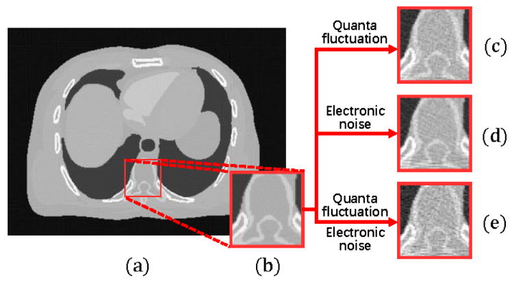
(a) An example of noise-free CT image. (b) The amplified illustration of the red box in (a). (c) The FBP reconstruction result with only simulated quanta fluctuation added to projection data. (d) The FBP reconstruction result with only simulated electronic noise added to projection data. (e) The FBP reconstruction result with both simulated quanta fluctuation and simulated electronic noise added to projection data.
To reconstruct high quality images from low-dose CT projection data, it is desirable to deal with both the aforementioned noise sources simultaneously. On one hand, the photon statistics can be well approximated as a Poisson distribution, whose variance ν equals to the mean μ, and thus it holds that . This implies that the ratio of standard deviation and mean of the distribution will approach infinity when the mean approaches zero (note that the degree of corruption should be measured by the ratio of standard deviation and mean instead of the ratio of variance and mean), and thus the noise will be very obvious when the mAs value in CT imaging is low. On the other hand, the electronic noise background has also been considered as an important factor affecting the image quality in low-dose CT imaging [26], [43]. This issue is especially critical in ultra low-dose situations when the quanta of the X-rays are close to the extent of the electronic noise. This makes the CT image very noisy and the highly mixed electronic noise becomes difficult to remove.
To address these two issues, many CT sinogram recovery (CTSR) methods have been proposed to estimate the ideal ones from the acquired noisy sinograms and then reconstruct the final high-quality CT image from the estimated ideal sinogram. They can be categorized into two main classes: the post-log and pre-log [12] methods. The post-log CTSR methods yield the desired CT image usually from the post-log restored sinogram data by statistical iterative algorithms [10], [22], [38], [39]. In particular, by assuming the mixed noise in the measured sinogram data as a Gaussian, a penalized weighted least-square (PWLS) function is typically used in most post-log CTSR methods [10], [38], [39]. Although PWLS possesses the advantage of easy computation attributed to its weighted least-square form, it fails to accurately use the Poisson-distribution-characteristic underlying the pre-logpre-lot projection data. Specifically, the logarithm operation on projection data can result in amplification of the noise, especially for low-dose CT imaging [14], and consequently cause positive recovery bias for E[−log(X)] ≥ −log(E[X]). Thus, approximation the noise simply as a Gaussian for the post-log sinogram data can hardly capture the actual statistical properties of data concealed by logarithm transform. In addition, estimation of the weights in the PWLS method is generally a challenging task due to the correction of non-positive values and the non-linearity of the logarithm [20]. Statistical correlation between the estimated weights and the noisy data can further cause negative bias in the reconstructed image.
On the other hand, the pre-log CTSR methods use the Beer-Lambert law to construct the forward model and directly recover pre-log projection data from the Poisson-distribution-assumption of the measurements [19]. Many pre-log algorithms are designed based on the Poisson noise model, such as the Penalized-likelihood (PL) method [9], [19], [31]. With appropriate statistical models, the pre-log CTSR regime can accommodate the non-positive values in the measurements. To further model electronic noise, the shifted Poisson [19], [31] and the Gaussian [19] models in the pre-log domain have also been adopted. However, these methods still consider the electronic noise background in a heuristically approximate way and do not fully inject the intrinsic statistical “Poisson+Gaussian” properties. It is generally considered a challenge to accurately model both properties in a theoretically sound manner. In this study, we develop a generative model (a general framework) describing an intrinsic CTSR mechanism that incorporates both statistical properties of photon statistics and electronic noise background.
In many of the previous works, some useful prior structure knowledge of the pre-log/post-log projection data are employed in the sinogram recovery models, which have been verified to play a critical role for successful low-dose CT sinogram recovery [6], [9], [11], [18], [22], [38]. Such prior knowledge is often encoded as a regularization term in the objective function. By utilizing such a prior information, the methods have always shown to be superior in better noise-induced artifacts suppression as compared to the traditional filtered-back- projection-based method without any treatments. One commonly utilized regularization is directly based on quadratic penalty model wherein the model is generally applied to simple difference of a sinogram sample with its horizontal (radial) and vertical (angular) neighbors [6], [9], [11], [18], [38]. However, this model does not consider applying asymmetric penalties to recovering the pre-log/post-log projection based on the intrinsic characteristics underlying the objective measurement, i.e., the different dimensions represent different physical or geometric quantities. Another commonly utilized regularization is based on non-quadratic penalty model, i.e., edge-preserving Huber penalty [6], [22]. Although this model can obtain noticeable improvements in resolution-variance tradeoffs compared to the conventional quadratic penalty model, the selection of the Huber parameter in the model is highly object size-dependent. In this study, we intend to design an advanced prior model which can more faithfully represent the underlying structures of post-log sinogram data as compared with the conventionally used ones.
In this paper we attempt to take full use of both the statistical properties of pre-log projection data and more accurate prior knowledge of post-log sinogram data to construct the statistical model for CTSR. In particular, this work contains the following three-fold contributions.
Instead of the heuristic or approximate manner of traditional CTSR techniques, a comprehensive CTSR model is proposed by properly encoding both the statistical properties of photons and the electronic noise background knowledge into one unique model. This model constitutes a general framework for describing intrinsic CTSR mechanism and can be easily extended to general cases of CTSR tasks. All parameters in the model, including the to-be-recovered sinogram and noise parameters, can be finely estimated by virtue of standard maximum a posteriori (MAP) framework.
A new prior model on sinogram data is proposed. As compared with the conventional priors utilized on sinogram data, the proposed prior delivers a more faithful representation for the underlying piecewise-linear structures of sinogram data, i.e., the sinogram manifold can be well approximated by combination of a series of flat surfaces in local areas.
An effective algorithm is designed for solving the model by using an extended alternating direction method of multipliers (ADMM) [2]. Each step in the algorithm can be efficiently implemented. Experimental on simulated and real low-dose CT data demonstrate the superiority of the proposed method according to both visual inspection and comprehensive quantitative performance evaluation.
II. Notions And Preliminaries
Denote Y ∈ ℝN as the vectorization of the matrix Y ∈ ℝm×n (where N = mn), and Yij be the element at the ith row and jth column of Y. Denote Z = [Zh, Zv] as the difference matrix of Y, where the elements of Zh and Zv are denoted by
respectively. Then we can introduce the difference operators Dh and Dv as
| (1) |
Since the difference operator is linear, we can denote the first order difference matrix D1 = ℝ2N×N and second order difference matrix D1 = ℝ4N×N, respectively, as follows:
| (2) |
Note that
| (3) |
where p > 0 is the shape parameter. || · ||TV is one of the most typical anisotropic version total variation (TV) norms, which is often used as the regularization term to deliver the smoothness prior in many image processing [4], [16], [32], [40] and CT denoising [8], [19], [24], [29] methods.
III. Model Formulation
In this section we will present the posterior distribution for a sinogram by simultaneously considering the statistical generative model of projection data and the prior knowledge of sinogram data, and then employ MAP to estimate all the parameters in the model.
A. Generative Model of Projection Data
We denote the sinogram data produced by the CT scan as a one-dimensional (1-D) vector Ỹ, with elements Ỹi = i, i = 1,…, N, where N is the total number of measurements in the scan. This number can be calculated as the product of the number of detector elements m and the number of projection views acquired n. By the Beer-Lambert Law, under clean circum- stances, the projection data can be obtained by
where I0i denotes the incident X-ray intensity along the projection path i.
In practice, the projection data P are generally mixed with noise. We then need to reformulate the generative model on P as the following mathematical expression in a more precise manner:
| (4) |
where Q ∈ ℕN denotes the quanta of rays received by detectors, and ε ∈ ℝN denote the electronic noise. Note that both terms deliver uncertainty, conducting possible sources of noise, to the projection P. The first follows X-ray photon statistics and the second leads to electronic noise background.
The electronic noise ε is caused by many latent factors and generally with not very large extent. Just as with conventional methods, we can rationally assume that it follows a Gaussian distribution:
| (5) |
where σ2 denotes the variance of noise, which can be obtained by standard procedures in modern CT systems.
The quanta of received rays Q can be considered as a perturbed result of the ideal quanta of rays caused by the inevitable quanta fluctuation of ray, which can be well depicted by a Poisson distribution [41] [19] as follows:
| (6) |
where O denotes the ideal quanta of rays, which is also the mean number of rays quanta.
Denote Y as the ideal sinogram which is the final target in our sinogram estimation model. According to the Beer- Lambert Law, it satisfies:
| (7) |
Combine (6) and (7), we can obtain the following conditional distribution:
| (8) |
From (5) we can obtain that
| (9) |
Thus, by combining (8) and (9), we can obtain the generative- model as the following conditional distribution:
| (10) |
Note that the statistical property of the photons and the electronic noise background have been considered by (8) and (9), respectively. The data generative model (10) thus describes the intrinsic mechanism underlying the ideal sinogram Y in a more accurate way than conventional models.
B. Prior of Sinogram
The ideal sinogram of a scan Y is generally a relatively smooth configuration, and many previous works easily model this smoothness as TV norm regularization (3) [6], [8], [19]. In this section, we will specifically consider the characteristics of sinogram data and construct a more appropriate prior form to facilitate a better CTSR performance.
From Fig. 2(a), we can see a distinguished feature of sinogram: it can be formed as a manifold (with respect to axis along detector elements and projection view) approximately constituted by a combination of flat surface in its local region. This means that it is better to describe the sinogram as a piecewise linear configuration rather than a piecewise constant one (as what the TV-norm represents). Thus, we can obtain that the second order derivative of sinogram will be very sparse (much more sparse than its first order derivative, as clearly demonstrated from Fig. 2(b)(c)), since the second order derivative of a linear flat is zero. This means that the TV regularization, representing the sparsity of the first order derivative, might not be the most proper one for describing such prior knowledge of the sinogram. For convenience, we call this distinguishing property of sinogram as the piecewise-linear prior.
Fig. 2.

(a) The manifold of an example sinogram data with axis along detector elements and projection views. The upper right is the illustration of the example sinogram. The upper left is the amplified area at a 2.5 times larger scale for easy observation of details; (b) and (c) are the absolute of the first and second order vertical derivatives calculated on the example sinogram, respectively, where the deeper the color is, the larger the value is. It can be observed from (a) that it is better to describe the sinogram as piecewise linear rather than piecewise constant (as what TV encourages). From (b) and (c), one can see that the second order derivative of a sinogram is evidently more sparse the first order one.
It is natural to use Hessian penalty [3], [35] to induce the sparsity of the second order derivative. In this work, we employ a new prior, related to Hessian penalty but easier to be calculated, to embed this prior into our model. We first introduce the following general distribution formulation, which can encode the transformed-sparsity of data:
| (11) |
where is the exponential power distribution (or Hyper-Laplace distribution) defined in [28], with b denoting the scale parameter, f:ℝN → ℝM is a linear operator dependent on specific requirements in different data, and cf is a constant with respect to the operator f. Eq. (11) can be used as a general formulation to model data when it is sparse after a proper transformation [16], [44].
It is easy to see that (11) can well describe the sparsity of the second order derivative of Y if we denote f(·) as following:
| (12) |
where D2 is the second order difference matrix as defined in Sec. II. In this case, we can see that this term can well encode the sparsity of the second order derivative of Y. For convenience of notation, we denote as TV2 in the following, which delivers its intrinsic meaning of the sparsity on data after two orders of TV transformation implemented on it.
By imposing the non-informative prior distribution p(b) (which is a constant function) of the parameter b, we can obtain the following prior distribution imposed on data:
| (13) |
Furthermore, the sparsity of D2Y, i.e., the piecewise-linear prior, can be finely delivered by (13). With this prior distribution, we can perform MAP estimation to estimate all parameters involved in the model.
C. Maximum A Posterior Estimation
By combining (10) and (13), we can obtain the entire posterior distribution on data as follows:
| (14) |
where p(P) is a constant for the observation P, and f(Y) is defined as (12). We can now estimate Y under the above MAP framework. Given the posterior distribution (14), our aim is to maximize its logarithm, i.e., solving the following optimization problem:
| (15) |
By employing Z = D2Y, (15) can be equivalently reformulated as:
| (16) |
which can be readily solved by applying the well-known ADMM strategy.
D. A Remark
In fact, if we assume the linear operator in (11) as follows:
where D1 is the first order difference matrix denoted in Sec. II, we can then obtain the prior expressed as:
| (17) |
Then, when we perform the MAP estimation, we can obtain the following regularization in our objective function:
This is exactly a special case of the nonconvex TV norm regularization as defined in (3), which has been used in many of the previous works. This shows that the proposed framework can be degenerated to the conventional case and also can be easily extended to a wider range of prior cases.
As one of the most popular statistical models, the MAP estimation is widely adopted in many of the current methods [8], [19], [27], with a specified likelihood function as well as priors imposed on the sinogram or the CT image. As compared with the previous MAP methods, the proposed method makes improvements in both the likelihood/loss function and the prior/regularization settings. On one hand, through fully encoding the statistical properties of the X-ray photons and the electronic noise background, the two sources intrinsically causing the noise in low-dose CT, the likelihood function of the problem can be more properly conducted in our method. On the other hand, as aforementioned, we use the piecewise linear regularization to more precisely represent the prior configuration underlying sinogram. In the following, we denote the proposed method as IMAP – TV2 (improved maximum a posteriori with sparsity on sinogram after two orders of TV transformation) for convenience.
IV. ADMM Algorithm
In this section, we solve (16) by using the ADMM scheme. The augmented Lagrangian function of (16) is
| (18) |
where Λ ∈ ℝM is the Lagrange multiplier and μ is a positive scalar.
With the other parameters fixed, the parameter Q can be updated by solving , which is equivalent to the following sub-problem:
| (19) |
This problem can be solved separately for each Qi as:
| (20) |
The solution can be obtained by Algorithm 1.
Algorithm 1.
Algorithm for Updating Q
| Input: Y, P, I0 and σ |
| 1: Initialize Q as the value of Q we obtained in the last step of complete algorithm, |
| 2: for i = 1:N do |
| 3: while h(Qi) > h(Qi + 1) do |
| 4: Update Qi = Qi + 1 |
| 5: end while |
| 6: while h(Qi) < h(Qi + 1) do |
| 7: Update Qi = Qi − 1 |
| 8: end while |
| 9: end for |
| Output: Q+ = Q |
With the other parameters fixed, the parameter Y can be updated by solving , which is equivalent to the following sub-problem:
| (21) |
This is a convex optimization problem and multiple off-the- shelf techniques can be easily used to find its global optimum. In our method, we use the framework of the accelerated first order method proposed in [1] to solve (21). By taking the quadratic approximation of the second term at a given point Ŷ(l), we can obtain the following approximate form of the objective function of (21):
| (22) |
where ⊙ denotes element-by-element multiplication, and the parameter τ can be taken as the largest element of I0. The key step in the framework is to solve , which is proved to have a closed-form solution [16]:
| (23) |
where ℱ(X) is defined as a 2D Fourier transform on X (X is the matrix form of X, i.e., X = vec(X) ), and || · ||1 is defined as the summation of the absolute values of all elements in a matrix. The entire algorithm for solving (21) is given in Algorithm 2.
Algorithm 2.
Algorithm for Updating Y
| Input: I, Z, Λ, μ and | |
| 1: | Initialize Ŷ(l) − Y(0) Ŷ(l) and t(1) = 1 complete algorithm, |
| 2: | for i = 1:L do |
| 3: | Update with (23) |
| 4: | Update |
| 5: | Update |
| 6: | end for |
| Output: Y+ = Y(l) | |
With the other parameters fixed, Z can be updated by solving , which is equivalent to the following sub-problem:
| (24) |
whose local optimum solution can be obtained in closed-form as: [37]:
| (25) |
Here Sλ(·) denotes a thresholding operator [44] defined as:
| (26) |
with .
With the other parameters fixed, b can be updated by solving , which is equivalent to the following sub-problem:
| (27) |
Let the derivative of the above function equal to 0, and then we can get the update equation for parameter b as follows:
| (28) |
The entire algorithm for solving (16) can be summarized in Algorithm 3. After obtaining the sinogram Y, the FBP method is introduced to reconstruct the CT image. In the algorithm, we set ρ a value close to 1 (e.g., ρ = 1.1), in order to prevent μ from increasing too fast, which may cause the issue that the iteration stops too quickly and is unable to achieve a good solution [21]. For the initial value of the penalty parameter μ, we easily set it as 100 throughout all our experiments. For most previous methods along this line of research, it is critical to select a proper trade-off parameter for compromising the likelihood/loss term and the prior/regularization terms. The proposed method has finely encoded this parameter (b in our algorithm) as a variable to be optimized in the MAP framework, and thus makes its selection from being manually specified to being automatically rectified from data. About its initialization, we just easily set it in the interval [1,2], and our method can then consistently perform well throughout all the experiments.
Algorithm 3.
IMAP-TV2 Algorithm for Solving (16)
| Input: P =I0 ⊙ e−Ytilde;, I0i | |
| 1: | Initialize μ, b, ρ, Λ = 0 and Y = max{ln(I0) − ln(P), 0} |
| 2: | while not convergence do |
| 3: | Update Q by Algorithm 1. |
| 4: | Update Y by Algorithm 2. |
| 5: | Update Z by (25) |
| 6: | Update b by (28) |
| 7: | Update Λ by Λ+ = Λ + μ(D2Y − Z) |
| 8: | Let μ = ρμ |
| 9: | end while |
| Output: the denoised scan Y | |
It should be noted that the proposed algorithm is a multi-block non-convex optimization algorithm. Unlike the basic form of ADMM [2] defined on convex problem with two- block variables, Algorithm 3 cannot be strictly proved to converge [5]. However, as empirically verified and discussed by many literatures, the effectiveness of the ADMM strategy has been widely substantiated in various machine learning and computer vision problems [30], [36]. We thus prefer to use the ADMM strategy in this work, which is easy to implement and consistently performs well in all our experiments to solve the problem.
V. Experimental Results
In this section, we test the performance of the proposed method, as compared with the previous CTSR methods on several simulated and real CT data.
A. Comparison Methods
To validate and evaluate the performance of the proposed method, the sinogram-domain PL [19], a typical and widely utilized pre-log method, PWLS [38], the state-of-the-art post- log method, and POCS-TV [34], a representative iterative image reconstruction method, are adopted. In addition, two more methods were utilized to evaluate the effectiveness of the data generative model (10) and the piece-wise linear prior (13), respectively. The first one is called IMAP-TV (maximum a posteriori with TV-norm regularization), with the proposed data generative model (10) while the classic TV-norm regularization term. This method facilitates us to evaluate the function of the piecewise-linear prior (10) in our method. The second one is called PWLS-TV 2, with the proposed piecewise-linear prior (13) and, instead of the proposed data generative model (10), has the following distribution:
| (29) |
This has the equivalent effect as the cost function of PWLS. Here Σ is a diagonal matrix as defined in [13]. This comparison method is used to evaluate the capability of the data generative model (10) involved in our method. The recovery by directly using FBP on the corrupted projection data is also compared. The method is easily denoted as FBP.
Extensive experiments with different parameter settings were tested for all competing methods, and the final result is specified for each method on the parameter with the largest the peak signal-to-noise ratio (PSNR) value to guarantee a fair comparison.
B. Digital Phantom Study
A modified digital XCAT phantom (shown in Fig. 3(a)) is used in this study [33]. The XCAT phantom consists of left ventricle, aorta, healthy myocardium, ischemic myocardium, and right ventricle were represented by the TACs. A simulation method [7], [19], was used to acquire the low-dose myocardial perfusion CT sinogram (MPCT) data. When we have the noise-free line integral Y, the noisy measurement Piat each bin i was generated according to the statistical model of pre-logarithm projection data (i.e., Eq. (4)), where the electronic background noise variance σ2 is set to be 11. The noise level related to the projection data with about 20 mAs at 80 kVp was simulated. In the simulation study, the simulated CT imaging parameters are the same as a clinical Siemens SOMATOM Sensation16 CT scanner: (i) the distance from the X-ray source to the detector arrays is 1040 mm and the distance from the X-ray source to rotation center is 570 mm; (ii) each rotation includes 1160 projection views that are evenly spanned on a 360° circular orbit; (iii) each view has 672 detector bins, and (iv) the space of each detector bin is 1.407 mm.
Fig. 3.
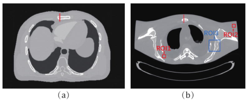
(a) illustration of the 1st frame of the noise-free digital myocardial perfusion phantom; (b) The noise-free image anthropomorphic torso phantom.
Fig. 4 shows the digital XCAT images reconstructed by all competing methods. From the results, it can be observed that the PL, PWLS-based, and MAP-based methods perform better than the FBP in terms of noise and artifacts suppression effects. It can be seen that the FBP results are evidently corrupted by severe noise-induced artifacts. For clear observation, the zoomed-in-views of two demarcated areas by different methods are also displayed. We can see that the results of PL, PWLS, POCS-TV, and PWLS- TV2 have non-uniform intensity distributions in the homogeneous area and some details are smoothed out, and the IMAP- TV and IMAP-TV2 can both well suppress noise-induced artifacts. Moreover, IMAP-TV2 achieves a better result in preserving spatial resolution than IMAP-TV. Furthermore, the vertical profiles at the pixel positions x = 245 and y from 155 to 180 shown in Fig. 5 demonstrate that the IMAP-TV2 achieves more noticeable gains than the other competing methods in preserving the edge details as compared with the ground truth.
Fig. 4.

(a) The noise-free digital XCAT image; (b)–(h) The images reconstructed by the FBP PL, PWLS, POCS-TV, PWLS-TV2, IMAP-TV and IMAP-TV2 methods at 20 mAs, respectively. The demarcated area in each image is amplified at a 3 time larger scale for easy observation.
Fig. 5.
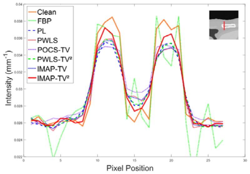
The vertical profiles of the noise-free image and recovery results of the 7 competing methods of digital XCAT images at 20 mAs. The vertical profiles is located at the pixel positions x = 245 and y from 155 to 180. as shown in Fig. 3(a).
To quantitatively substantiate the advantage of the proposed method, Table I lists three measurement of the low-dose CT recovery, including PSNR, feature similarity (FSIM) [46], and normalized-mean-square error (NMSE), obtained by all competing methods. PSNR and NMSE are two conventional quantitative picture quality indices, and FSIM emphasizes the perceptual consistency with the reference image. The larger PSNR and FSIM are, the closer the target image is to the reference one. Contrarily, the smaller the NMSE is, the better the reconstructed result is. From these results, the advantage of the proposed method can be evidently observed. Specifically, our method can outperform other competing methods in terms of all these evaluation measures.
TABLE I.
PSNR, FSIM, and RMSE measurements of the digital XCAT images reconstructed by all. competing methods
| FBP | PL | PWLS | POCS-TV | PWLS-PL | IMAP-TV | IMAP-TV2 | |
|---|---|---|---|---|---|---|---|
| PSNR | 19.91 | 32.95 | 33.66 | 34.86 | 34.25 | 34.63 | 35.34 |
| FSIM | 0.687 | 0.932 | 0.931 | 0.953 | 0.940 | 0.947 | 0.958 |
| NMSE | 0.326 | 0.068 | 0.064 | 0.056 | 0.059 | 0.056 | 0.052 |
|
| |||||||
| Time (s) | 24.4 | 26.7 | 26.9 | 698.2 | 36.9 | 27.8 | 30.4 |
By comparing the results of IMAP-TV2 and PWLS-TV2, it can be seen that the data generative model (10) and its exactly solver can help enhance a notable improve the noise reduction performance. By comparing the results of IMAP-TV 2 and IMAP-TV, it can be seen that the developed piecewise- linear prior (13) can also help improve the noise reduction performance both in finer-grained textures and coarser-grained structures recovery. This substantiates the rationality of both of the two terms designed in the proposed MAP model for the problem.
C. Physical Phantom Study
The phantom was scanned by a clinical CT scanner (Siemens SOMATOM Sensation 16 CT) at five exposure levels, i.e., 17, 40, 60, and 100 mAs, with the tube voltage set at 120 kVp, and the phantom was scanned in a cine mode at a fixed bed position. The associated imaging parameters of the CT scanner are the same as the one in the digital phantom study. Fig. 3(b) shows the CT image reconstructed by the FBP method with ramp filter from the averaged sinogram data of 150 repeatedly measured samples acquired at 100 mAs and 120 kVp, which is used as the ground truth for comparison.
From Fig. 6, it is easy to observe the fine noise-suppression-capability of the proposed method. Fig. 7 depicts the associative vertical profiles across the 160th to 190th rows at the 240th column from the results at 17 mAs. It can be observed that the profiles of the results from IMAP-TV2 are closer to that of the ground truth image than those from other methods. This further reflects that our method has a better noise reduction capability while protecting both the finer-grained textures and coarser-grained structures. Fig. 8 illustrates the normal vector flow (NVF) images [23] of the recovery results at the position of image shown as ROI 3 in Fig. 3. The NVF expresses the gradient vectors of the original image at each location as arrows, while noise is often shown as disordered arrows. As we can observe from Fig. 8, the NVF of IMAP-TV2 is the closest to the noise-free image among all of the completed sinogram recovery methods, i.e., the arrows in homogeneous area are closer to zero and the arrows at the edge of areas are less messy. Fig. 9 shows the residual of reconstructed results1 obtained by all methods. We can observe that the proposed IMAP-TV2 method can better suppress noise-induced artifacts than other methods with fewer edge detail loss.
Fig. 6.

(a) The noise-free image of the anthropomorphic torso phantom study; (b)–(h) The images reconstructed by FBP. PL, PWLS, POCS-TV, PWLS-TV2, IMAP-TV and IMAP-TV2 at 17 mAs, respectively. The demarcated area in each image is amplified at a 3 time larger scale for easy observation of details.
Fig. 7.
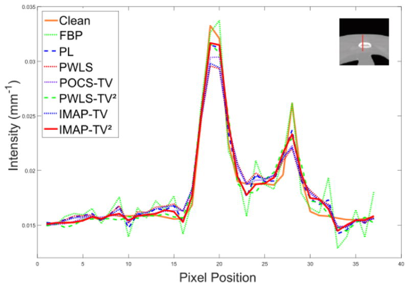
The vertical profiles of the noise-free image and recovery result of the 7 methods of digital anthropomorphic torso phantom at 17 mAs. The vertical profiles is located at the pixel positions x = 240 and y from 160 to 195. as shown in Fig. 3(b).
Fig. 8.
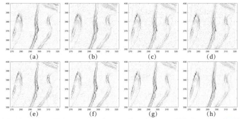
The NVF images at the position shown as ROI 3 in Fig. 3(b), (a) noise-free image, (b)–(h) the results reconstructed by FBP, PL, PWLS, POCS-TV, PWLS-TV2, IMAP-TV and IMAP-TV2.
Fig. 9.
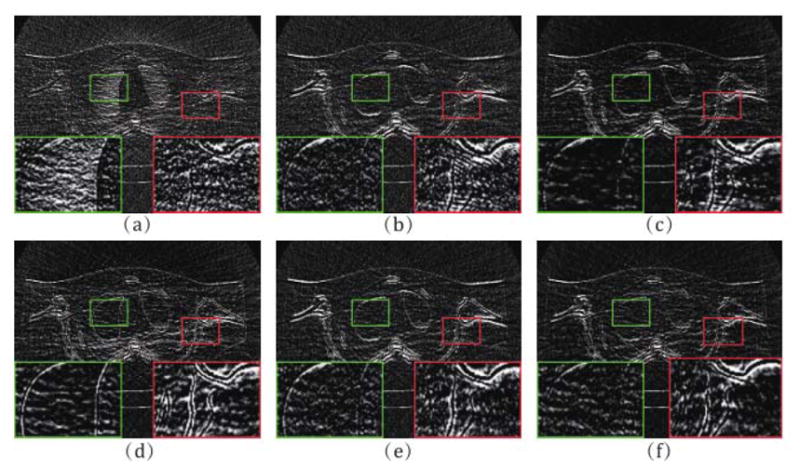
(a)–(f) Residuals of the result reconstructed by PL, PWLS, POCS-TV, PWLS-TV2, IMAP-TV, IMAP-TV2 at 17 mAs, respectively.
To quantitatively evaluate the noise reduction performance of the presented IMAP – TV2 method, the PSNR, FSIM and NMSE on the recovery results by all competing methods were measured at 17 mAs, 40 mAs and 60 mAs, respectively, and the results are listed in Table II. It can be observed that the presented IMAP – TV2 method achieves the highest PSNR and FSIM, lowest NMSE values among all completing sinogram recovery methods in all cases. Moreover, the numerical results of IMAP − TV2 are comparable to the iterative image reconstruction method POCS-TV at 40 mAs and 60 mAs, and are better than POCS-TV at 17 mAs. Considering that the POCS-TV method requires significantly more computational cost than other sinogram recovery methods, it should be rational to say that the proposed method is more efficient. Fig. 10 shows the means and standard deviations in two homogeneous areas (ROI1 and ROI2 in Fig. 3) reconstructed by PL, PWLS, POCS-TV, PWLS-TV2, IMAP-TV and IMAP-TV2 methods, respectively. It can be seen that the proposed method can achieve a smaller standard deviation with a mean value closer to the noise-free data, as compared with the competing methods. The experimental results demonstrate that the proposed IMAP-TV2 method can achieve about 80% noise reduction in conventional CT imaging research and further demonstrates the effectiveness of the proposed methods in both noise/artifacts suppression and CT recovery.
TABLE II.
PSNR FSIM and NMSE measurements obtained by the all competing methods at different doses on anthropomorphic torso phantom data
| dose | FBP | PL | PWLS | POCS-TV | PWLS-TV2 | IMAP-TV | IMAP-TV2 | |
|---|---|---|---|---|---|---|---|---|
| PSNR | 17 mAs | 27.83 | 36.12 | 36.20 | 37.89 | 37.34 | 37.45 | 38.42 |
| 40 mAs | 31.96 | 38.02 | 38.04 | 40.62 | 39.82 | 39.06 | 40.67 | |
| 60 mAs | 33.95 | 39.08 | 39.21 | 41.80 | 40.87 | 40.14 | 41.74 | |
|
| ||||||||
| FSIM | 17 mAs | 0.884 | 0.958 | 0.963 | 0.968 | 0.968 | 0.969 | 0.975 |
| 40 mAs | 0.935 | 0.973 | 0.976 | 0.984 | 0.980 | 0.979 | 0.984 | |
| 60 mAs | 0.953 | 0.979 | 0.981 | 0.988 | 0.983 | 0.984 | 0.988 | |
|
| ||||||||
| NMSE | 17 mAs | 0.189 | 0.0723 | 0.072 | 0.059 | 0.063 | 0.066 | 0.056 |
| 40 mAs | 0.117 | 0.058 | 0.059 | 0.043 | 0.047 | 0.054 | 0.043 | |
| 60 mAs | 0.093 | 0.052 | 0.051 | 0.038 | 0.042 | 0.047 | 0.038 | |
|
| ||||||||
| Mean Time (s) | 24.5 | 25.9 | 25.5 | 671.1 | 35.4 | 26.8 | 29.3 | |
Fig. 10.
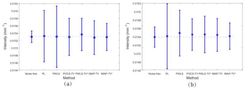
Comparison of ROI reconstructed by the 6 competing methods.
D. Preclinical Porcine Data Study
Approved by the Animal Care Committee at the Tianjin Medical University General Hospital (Tianjin, China), a healthy Chinese minipig (weight 22.5 kg, female) was used in this study. In the experiment, a cuffed endotracheal tube with inner diameter of 4.5 mm was placed in the trachea for anesthesia inspiration and respiration after an intramuscular injection of ketamine (20mg/kg), xylazine hydrochloride (1.5mg/kg), and atropine (0.02mg/kg) was performed in premedication. With the support of the animal anespirator (Matrx VMS Plus VMC, Anesthesia Machines, Midmark, New York), the pig was mechanically ventilated and anaesthetized with sevoflurane (2.5%–3.5% in oxygen) during the angioplasty and myocardial perfusion CT scanning. Similar to the previous study [45], the acute myocardial infarction in the pig was constructed with an angioplasty balloon, and corresponding measured projection data are acquired from a 64-slice multi-detector GE Discovery CT750 HD scanner in cine mode with following protocol: 120 kVp and 100 mAs per rotation with a total scan duration of about 30s. From the acquired high-dose myocardial perfusion CT data, we can simulate the low-dose CT data at 20 mAs similar to the previous section.
Fig. 11 shows the high-dose and low-dose preclinical porcine data reconstructed by different algorithms at the 8th frame. We can observe that the proposed IMAP-TV2 method can obtain evidently closer image feature representation with the high-dose one than other competing methods, especially in the myocardium region as indicated by the red rectangle. To further demonstrate the performance of the proposed IMAP- TV2 method, the hemodynamic perfusion parameters, i.e., myocardial blood flow (MBF), are introduced wherein the MBF can be used to reflect the qualitative assessment of blood supply and calculated by the block-Circulant Singular Value Decomposition (bSVD) algorithm [42]. The corresponding results are illustrated in Fig. 12. From the results, it can be observed that the proposed IMAP-TV2 method can produce gains over other competing methods in accurate MBF estimation by visual inspection, especially in the ischemic myocardium region indicated by yellow arrows. In addition, the selective demarcated areas as indicated by the green rectangles also demonstrate the effectiveness of the proposed method in improving the hemodynamic perfusion parameters estimation accuracy.
Fig. 11.

(a) The high-dose image of the 11th frame of preclinical porcine data; (b)–(h) The images reconstructed by the FBP, PL, PWLS, POCS-TV, PWLS-TV2, IMAP-TV and IMAP-TV2 methods at 20 mAs, respectively. The demarcated area in each image is amplified at a 3 time larger scale for easy observation.
Fig. 12.

(a) The MBF maps from high-dose images; (b)–(h) The MBF maps from simulated low-dose images reconstructed by FBP, PL, PWLS, POCS-TV, PWLS-TV2. IMAP-TV and IMAP-TV2 methods, respectively. The demarcated area in each image is amplified at a 3 time larger scale for easy observation.
VI. Conclusion
In order to make full use of the statistical properties of projection data, this paper has proposed a MAP based CTSR framework, which can encode the two major sources to CT data noise, i.e., the X-ray photon statistics and the electronic noise background, in a statistically sound manner and perform data denoising based on the noise generation mechanism of sinogram data. Furthermore, we construct a new piecewise linear prior to better encode the structure of the sinogram. Differing from the traditionally utilized regularization terms, the proposed piecewise linear prior takes the special structure of sinogram into consideration, i.e., the correlated manifold can be approximately constituted by a combination of several flat surfaces. All of the involved parameters in the model can be automatically estimated in our method, including the trade-off parameter for compromising between the loss term and the regularization term in the model. An effective ADMM method is constructed to solve the proposed model, whose superiority is demonstrated by a series of experimental results on low-dose CT data recovery.
The proposed work also suggests other interesting points meriting future study since the MAP framework can be generally adopted to other CT recovery problems, including that on 3D multi-slice CT data. 3D multi-slice data contain more sufficient knowledge which possibly facilitates a more comprehensive model with better sinogram recovery capability, especially for the prior term, which should supplementally encode the information of correlations among slices besides the 2D piecewise linear knowledge. By still adopting the likelihood term as proposed in this study while using such enhanced prior term, the proposed model can be easily extended to be used for multi-slice data. Since we have substantiated the properness of both of the proposed likelihood and prior formulations in the 2D cases, we believe it should also be helpful in the 3D cases. Besides, it is meaningful to investigate how to accurately encode the compound Poisson statistics instead of its approximation in the proposed MAP model. We will explore these issues in our future research.
Acknowledgments
This work was supported by the National Natural Science Foundation of China project under Grant Nos. 61373114, 61661166011, 11690011, 61603292, 81371544 61571214, the National Grand Fundamental Research 973 Program of China under Grant No. 2013CB329404 and Macau Science and Technology Development Funds under Grant No. 003/2016/AFJ. DZ and ZB were partially supported by the China Postdoctoral Science Foundation funded project under Grant Nos. 2016M602489, 2016M602488, and the Guangdong Natural Science Foundation under Grant No. 2015A030313271. ZL was partially supported by the National Institutes of Health under Grant No. R01 CA206171.
We would like to gratefully thank Dr. Marc Pomeroy for his help on polishing the entire paper. We also would like to sincerely thank the anonymous reviewers for their constructive and valuable comments, which have helped us largely improve the quality of the paper.
Footnotes
Clculateda by E = |X0 − Xrecovery|
Contributor Information
Qi Xie, School of Mathematics and Statistics and Ministry of Education Key Lab of Intelligent Networks and Network Security, Xi’an Jiaotong University, Shaanxi, 710049, China.
Dong Zeng, School of Biomedical Engineering, Southern Medical University, Guangzhou 510515, China; and Guangzhou Key Laboratory of Medical Radiation Imaging and Detection Technology, Southern Medical University, Guangzhou 510515, China.
Qian Zhao, School of Mathematics and Statistics and Ministry of Education Key Lab of Intelligent Networks and Network Security, Xi’an Jiaotong University, Shaanxi, 710049, China.
Deyu Men, School of Mathematics and Statistics and Ministry of Education Key Lab of Intelligent Networks and Network Security, Xi’an Jiaotong University, Shaanxi, 710049, China.
Zongben Xu, School of Mathematics and Statistics and Ministry of Education Key Lab of Intelligent Networks and Network Security, Xi’an Jiaotong University, Shaanxi, 710049, China.
Zhengrong Liang, Departments of Radiology and Biomedical Engineering, Stony Brook University, Stony Brook, New York 11794, USA.
Jianhua Ma, School of Biomedical Engineering, Southern Medical University, Guangzhou 510515, China; and Guangzhou Key Laboratory of Medical Radiation Imaging and Detection Technology, Southern Medical University, Guangzhou 510515, China.
References
- 1.Beck A, Teboulle M. A fast iterative shrinkage-thresholding algorithm for linear inverse problems. Siam Journal on Imaging Sciences. 2009;2(1):183–202. [Google Scholar]
- 2.Boyd S, Parikh N, Chu E, Peleato B, Eckstein J. Distributed optimization and statistical learning via the alternating direction method of multipliers. Foundations & Trends in Machine Learning. 2011;3(1):1–122. [Google Scholar]
- 3.Boyd VLS. Convex optimization. Cambridge university press; 2004. [Google Scholar]
- 4.Chambolle A, Lions PL. Image recovery via total variation minimization and related problems. Numerische Mathematik. 1997;76(2):167–188. [Google Scholar]
- 5.Chen C, He B, Ye Y, Yuan X. The direct extension of admm for multi-block convex minimization problems is not necessarily convergent. Mathematical Programming. 2016;155(1):57–79. [Google Scholar]
- 6.Cui X, Gui Z, Zhang Q, Liu Y, Ma R. The statistical sonogram smoothing via adaptive-weighted total variation regularization for low-dose x-ray ct. Optik - International Journal for Light and Electron Optics. 2014;125(18):5352–5356. [Google Scholar]
- 7.Dong Z, Huang J, Bian Z, Niu S. A simple low-dose x-ray ct simulation from high-dose scan. IEEE Transactions on Nuclear Science. 2015;62(5):2226. doi: 10.1109/TNS.2015.2467219. [DOI] [PMC free article] [PubMed] [Google Scholar]
- 8.Fessler JA. Statistical image reconstruction methods for transmission tomography. Handbook of Medical Imaging, Volume 2. Medical Image Processing and Analysis. 2000 [Google Scholar]
- 9.Forthmann P, Köhler T, Begemann PG, Defrise M. Penalized maximum-likelihood sinogram restoration for dual focal spot computed tomography. Physics in Medicine & Biology. 2007;52(15):4513–4523. doi: 10.1088/0031-9155/52/15/010. [DOI] [PubMed] [Google Scholar]
- 10.Forthmann P, Koehler T, Defrise M, La RP. Comparing implementations of penalized weighted least-squares sinogram restoration. Medical Physics. 2010;37(11):5929–38. doi: 10.1118/1.3490476. [DOI] [PMC free article] [PubMed] [Google Scholar]
- 11.Forthmann P, Rivire PJL. Comparison of three sonogram restoration methods. Proceedings of SPIE - The International Society for Optical Engineering; 2006. [Google Scholar]
- 12.Fu L, Lee TC, Kim SM, Alessio A, Kinahan P, Chang Z, Sauer K, Kalra M, De MB. Comparison between pre-log and post-log statistical models in ultra-low-dose ct reconstruction. IEEE Transactionson Medical Imaging. 2016 doi: 10.1109/TMI.2016.2627004. PP(99):1–1. [DOI] [PMC free article] [PubMed] [Google Scholar]
- 13.Gao Y, Bian Z, Huang J, Zhang Y, Niu S, Feng Q, Chen W, Liang Z, Ma J. Low-dose x-ray computed tomography image reconstruction with a combined low-mas and sparse-view protocol. Optics Express. 2014;22(12):15190–210. doi: 10.1364/OE.22.015190. [DOI] [PMC free article] [PubMed] [Google Scholar]
- 14.Hsieh J. Adaptive streak artifact reduction in computed tomography resulting from excessive x-ray photon noise. Medical Physics. 1998;25(11):2139–2147. doi: 10.1118/1.598410. [DOI] [PubMed] [Google Scholar]
- 15.Hsieh J. Computed tomography: principles, design, artifacts, and recentadvances. SPIE; Bellingham, WA: 2009. [Google Scholar]
- 16.Krishnan D, Fergus R. Fast image deconvolution using hyper-laplacian priors. in nips. Advances in Neural Information ProcessingSystems 22: Conference on Neural Information Processing Systems 2009; Proceedings of A Meeting; 7–10 December 2009; Vancouver, British Columbia, Canada. 2009. pp. 1033–1041. [Google Scholar]
- 17.La Rivière P. Reduction of noise-induced streak artifacts in x-ray ct through penalized-likelihood sinogram smoothing. Conf Rec IEEE NSS-MIC. 2003 doi: 10.1109/tmi.2004.838324. [DOI] [PubMed] [Google Scholar]
- 18.La Riviere PJ. Penalized-likelihood sinogram smoothing for low-dose ct. Medical physics. 2005;32(6):1676–1683. doi: 10.1118/1.1915015. [DOI] [PubMed] [Google Scholar]
- 19.La Rivière PJ, Bian J, Vargas PA. Penalized-likelihood sonogram restoration for computed tomography. IEEE Transactions on Medical Imaging. 2006;25(8):1022–1036. doi: 10.1109/tmi.2006.875429. [DOI] [PubMed] [Google Scholar]
- 20.Lee TC, Zhang R, Alessio AM, Fu L, Man BD, Kinahan PE. Statistical distributions of ultra-low dose ct sinograms in the data processing stream. International Meeting on Image Formation in X-Ray Ct. 2016 [Google Scholar]
- 21.Lin Z, Chen M, Ma Y. The augmented lagrange multiplier method for exact recovery of corrupted low-rank matrices. 2010 arXiv preprint arXiv:1009.5055. [Google Scholar]
- 22.Little KJ, Rivire PJL. Sinogram restoration in computed tomography with a non-quadratic, edge-preserving penalty. 2012:2534–2536. doi: 10.1118/1.4907968. [DOI] [PMC free article] [PubMed] [Google Scholar]
- 23.Liu Y, Liang Z, Ma J, Lu H, Wang K, Zhang H, Moore W. Total variation-stokes strategy for sparse-view x-ray ct image reconstruction. IEEE Transactions on Medical Imaging. 2014;33(3):749–763. doi: 10.1109/TMI.2013.2295738. [DOI] [PMC free article] [PubMed] [Google Scholar]
- 24.Liu Y, Ma J, Fan Y, Liang Z. Adaptive-weighted total variation minimization for sparse data toward low-dose x-ray computed tomography image reconstruction. Physics in Medicine & Biology. 2012;57(23):7923–56. doi: 10.1088/0031-9155/57/23/7923. [DOI] [PMC free article] [PubMed] [Google Scholar]
- 25.Lu H, Hsiao T, Li X, Liang Z. Noise properties of low-dose ct projections and noise treatment by scale transformations. Nuclear Science Symposium Conference Record, 2001 IEEE; IEEE; 2001. pp. 1662–1666. [Google Scholar]
- 26.Ma J, Liang Z, Fan Y, Liu Y, Huang J, Chen W, Lu H. Variance analysis of x-ray ct sinograms in the presence of electronic noise background. Medical Physics. 2012;39(7):4051–4065. doi: 10.1118/1.4722751. [DOI] [PMC free article] [PubMed] [Google Scholar]
- 27.Ma J, Zhang H, Gao Y, Huang J, Liang Z, Feng Q, Chen W. Iterative image reconstruction for cerebral perfusion ct using a pre-contrast scan induced edge-preserving prior. Physics in medicine and biology. 2012;57(22):7519. doi: 10.1088/0031-9155/57/22/7519. [DOI] [PMC free article] [PubMed] [Google Scholar]
- 28.Mineo AM, Ruggieri M. A software tool for the exponential power distribution: The normalp package. Journal of Statistical Software. 2005;12(i04):1–24. [Google Scholar]
- 29.Penfold SN, Schulte RW, Censor Y, Rosenfeld AB. Total variation superiorization schemes in proton computed tomography imagereconstruction. Medical Physics. 2010;37(11):5887–5895. doi: 10.1118/1.3504603. [DOI] [PMC free article] [PubMed] [Google Scholar]
- 30.Peng Y, Ganesh A, Wright J, Xu W, Ma Y. Rasl: Robust alignment by sparse and low-rank decomposition for linearly correlated images. CVPR. 2010:763–770. doi: 10.1109/TPAMI.2011.282. [DOI] [PubMed] [Google Scholar]
- 31.Rivie’re PJL. Penalized-likelihood sinogram smoothing for low-dose ct. Medical Physics. 2005;32(6):1676–1683. doi: 10.1118/1.1915015. [DOI] [PubMed] [Google Scholar]
- 32.Rudin LI, Osher S, Fatemi E. Nonlinear total variation based noise removal algorithms. Physica D Nonlinear Phenomena. 1992;60(1C4):259–268. [Google Scholar]
- 33.Segars WP, Sturgeon G, Mendonca S, Grimes J, Tsui BMW. 4d xcat phantom for multimodality imaging research. Medical Physics. 2010;37(9):4902. doi: 10.1118/1.3480985. [DOI] [PMC free article] [PubMed] [Google Scholar]
- 34.Sidky EY, Pan X. Image reconstruction in circular cone-beam computed tomography by constrained, total-variation minimization. Physics in Medicine & Biology. 2008;53(17):4777–4807. doi: 10.1088/0031-9155/53/17/021. [DOI] [PMC free article] [PubMed] [Google Scholar]
- 35.Sun T, Sun N, Wang J, Tan S. Iterative cbct reconstruction using hessian penalty. Physics in Medicine & Biology. 2015;60(5):1965–87. doi: 10.1088/0031-9155/60/5/1965. [DOI] [PubMed] [Google Scholar]
- 36.Tao M, Yuan X. Society for Industrial and Applied Mathematics. 2011. Recovering Low-Rank and Sparse Components of Matrices from Incomplete and Noisy Observations. [Google Scholar]
- 37.Tibshirani R. Regression shrinkage and selection via the lasso: A retrospective. Journal of the Royal Statistical Society. 2011;73(3):273–282. [Google Scholar]
- 38.Wang J, Li T, Lu H, Liang Z. Penalized weighted least-squares approach to sinogram noise reduction and image reconstruction for low-dose x-ray computed tomography. IEEE Transactions on Medical Imaging. 2006;25(10):1272–1283. doi: 10.1109/42.896783. [DOI] [PMC free article] [PubMed] [Google Scholar]
- 39.Wang J, Liang Z, Lu H. Multiscale penalized weighted least-squares sinogram restoration for low-dose x-ray computed tomography. IEEE Transactions on Bio-medical Engineering. 2008;55(3):1022–31. doi: 10.1109/TBME.2007.909531. [DOI] [PubMed] [Google Scholar]
- 40.Wang Y, Yang J, Yin W, Zhang Y. A new alternating minimization algorithm for total variation image reconstruction. Siam Journal on Imaging Sciences. 2008;1(3):248–272. [Google Scholar]
- 41.Whiting BR, Massoumzadeh P, Earl OA, OSullivan JA, Snyder DL, Williamson JF. Properties of preprocessed sonogram data in x-ray computed tomography. Medical physics. 2006;33(9):3290–3303. doi: 10.1118/1.2230762. [DOI] [PubMed] [Google Scholar]
- 42.Wu O, OL, Weisskoff RM, Benner T, Rosen BR, Sorensen AG. Tracer arrival timing-insensitive technique for estimating flow in mr perfusion-weighted imaging using singular value decomposition with a block-circulant deconvolution matrix. Magnetic Resonance in Medicine. 2003;50(1):164C174. doi: 10.1002/mrm.10522. [DOI] [PubMed] [Google Scholar]
- 43.Xu J, Tsui BM. Electronic noise modeling in statistical iterative reconstruction. IEEE Transactions on Image Processing. 2009;18(6):1228–1238. doi: 10.1109/TIP.2009.2017139. [DOI] [PMC free article] [PubMed] [Google Scholar]
- 44.Xu Z, Chang X, Xu F, Zhang H. 1 1/2 regularization: A thresholding representation theory and a fast solver. IEEE Transactions on Neural Networks & Learning Systems. 2012;23(7):1013. doi: 10.1109/TNNLS.2012.2197412. [DOI] [PubMed] [Google Scholar]
- 45.Zeng D, Gong C, Bian Z, Huang J, Zhang X, Zhang H, Lu L, Niu S, Zhang Z, Liang Z. Robust dynamic myocardial perfusion ct deconvolution for accurate residue function estimation via adaptive-weighted tensor total variation regularization: a preclinical study. Physics in Medicine & Biology. 2016;61(22):8135–8156. doi: 10.1088/0031-9155/61/22/8135. [DOI] [PMC free article] [PubMed] [Google Scholar]
- 46.Zhang L, Zhang L, Mou X, Zhang D. Fsim: a feature similarity index for image quality assessment. IEEE Trans Image Processing. 2011;20(8):2378–2386. doi: 10.1109/TIP.2011.2109730. [DOI] [PubMed] [Google Scholar]