Next Generation Quality: Assessing the Physician in Clinical History Completeness and Diagnostic Interpretations Using Funnel Plots and Normalized Deviations Plots in 3,854 Prostate Biopsies

Abstract

Background:

Observational data and funnel plots are routinely used outside of pathology to understand trends and improve performance.

Objective:

Extract diagnostic rate (DR) information from free text surgical pathology reports with synoptic elements and assess whether inter-rater variation and clinical history completeness information useful for continuous quality improvement (CQI) can be obtained.

Methods:

All in-house prostate biopsies in a 6-year period at two large teaching hospitals were extracted and then diagnostically categorized using string matching, fuzzy string matching, and hierarchical pruning. DRs were then stratified by the submitting physicians and pathologists. Funnel plots were created to assess for diagnostic bias.

Results:

3,854 prostate biopsies were found and all could be diagnostically classified. Two audits involving the review of 700 reports and a comparison of the synoptic elements with the free text interpretations suggest a categorization error rate of <1%. Twenty-seven pathologists each read >40 cases and together assessed 3,690 biopsies. There was considerable inter-rater variability and a trend toward more World Health Organization/International Society of Urologic Pathology Grade 1 cancers in older pathologists. Normalized deviations plots, constructed using the median DR, and standard error can elucidate associated over- and under-calls for an individual pathologist in relation to their practice group. Clinical history completeness by submitting medical doctor varied significantly (100% to 22%).

Conclusion:

Free text data analyses have some limitations; however, they could be used for data-driven CQI in anatomical pathology, and could lead to the next generation in quality of care.

INTRODUCTION

Traditional inter-rater variation studies in pathology utilize a set of cases that are reviewed by a number of pathologists. These types of studies allow one to directly compare the interpretations of the participating pathologists, and assess inter-rater variation with a kappa value. If the study set is assessed by an expert or a panel of experts the interpretative bias of individual pathologists can be determined (in relation to a gold standard). These types of studies are important and may be particularly informative for the participants but likely have limited utility in a practice setting and may be biased by the study set selected.

Clinical data, in sufficient quantities, can provide another perspective on interpretive bias. In (non-pathology) clinical practice, where diagnostic decisions cannot be revisited, comparisons are made between providers on the basis of the population served. One well-established metric is provider caesarian section rate. It is tracked and compared among health-care institutions.[1] In surgery, it is typical to examine postoperative complications and infections, on a per provider basis. This allows the identification of outliers or unusual data points more quickly and may help identify suboptimal care. The underlying basis for these types of analyses is the following two assumptions:

1. The population served has disease characteristics that are stable, i.e., the incidence and severity of disease is stable over time

2. Care providers are not biased in their patient selection, in relation to their peers.

If both #1 and #2 are true and there is a sufficient case volume, stratification on the basis of care provider should yield the same event rates.

In pathology, clinical data are not widely used to compare diagnostic interpretation. Yet, one would expect that both assumptions #1 and #2 would be valid in most pathology practice settings. In many practice settings, pathologists do not actively choose the cases they read; the cases just land on their “to do” pile.

The main barrier to these analyses has been retrieving the data and categorizing it in a way that allows comparisons. Many pathology reports are still free text, and often not readily amenable to automated analyses due to a lack of standardized diagnostic terminology and lacking tools/resources typically available within pathology departments.

Free text reports can be analyzed to extract diagnostic categorization; however, these categorizations are (1) imperfect and (2) generally not done due to technical barriers. The accuracy of free text interpretations in pathology varies substantially; it can be nearly perfect (99% accurate) or be quite poor (65%).[2] Seen practically, in the context of analyzing free-text pathology reports, this may limit analysis work on conditions that have a prevalence lower than the error rate.

Comparisons between providers made on the basis of a common served population are subject to sampling error which is dependent on the sample size. The sample size limits the size of the interpretation bias that can be confidently detected.

Considered from a theoretical perspective, the measured diagnostic rates (DRs) calculated from the assessment of a randomly selected sample is dependent on (1) the ideal DR in the population (assumed to be constant over time), (2) sampling error, and (3) physician diagnostic bias.

If one assumes the null hypothesis of no diagnostic bias, the mean or median DR (of the pathologist group) estimates the ideal DR and all measurement variation represents the sampling error. One can then construct confidence intervals around the mean or median DR and assess the likelihood that a given physician's DR is influenced only by sampling error (null hypothesis true, diagnostic bias absent) or unlikely to be only sampling error (null hypothesis false, diagnostic bias present).

If one plots the DR versus the sample size and appropriately calculates the confidence interval (based on the sample size), one gets a funnel-shaped plot that is wide for small sample sizes and narrow for large sample sizes. This process (“funnel plots”) has been used in meta-analyses to detect publication bias. In the quality of care realm, it was described by Spiegelhalter in 2005.[3] It has been applied to cesarean section rate comparisons between institutions[1] and has found its way into the surgery literature, where it has been suggested it could be used to compare individual practitioners.[4] To the best of our knowledge, funnel plots have not been used in anatomical pathology to compare practitioner diagnostic call rates.

This work set out to assess whether (1) the pathologist DRs can be extracted and (2) if the rate data provides useful information regarding the hypothesis testing of no diagnostic bias.

With regard to prostate cancer grading, which is a significant determinant of management, this work sought to examine:

1. The World Health Organization (WHO)/International Society of Urologic Pathology (ISUP) (prognostic) grade group categorization rates on a pathologist basis

2. Compare WHO/ISUP grading done with different assumptions.

In our practice and the surrounding area, the WHO/ISUP grade (that is used to help determine treatment) is predominantly based on a summary score (hence referred to as Method S, for summary); it is generated by considering all cores as one piece of tissue. This differs from the practice more typical in some other jurisdictions; there, the WHO/ISUP score is based of the highest grade in the biopsy set (hence referred to as Method H, for highest).

This study also sought to examine the clinical history completeness on pathology requisitions, based on the submitting physician.

METHODS

All surgical pathology reports from two large teaching institutions (St. Joseph's Healthcare Hamilton, Juravinski Cancer Centre) were extracted through text dump from the Laboratory Information System (LIS) for a 6-year period (January 2011–December 2016), after research ethics board approval was obtained (Hamilton Integrated Research Ethics Board (HiREB) reference # 2017-3110).

The text dumps were structured and subdivided the reports into separate sections and included all information needed for the study. All patient identifiers were irreversibly removed from all the reports to ensure patient confidentially. Source files with patient identifiers were securely deleted with “shred” (gnu.org/s/coreutils). The surgical case numbers were preserved as a linkage to the LIS, so cases could be retrieved in the context of significant report deficiencies.

The scrubbed data dumps were then serially read by a custom interpreter that identified the individual surgical cases, subdivided them into their sections (e.g., source of specimen, gross, micro, diagnosis, cancer care summary/synoptic report, addendum), and extracted submitting medical doctor (MD) and assigned pathologist.

Prostate biopsy cases were retrieved with a complex search over several fields in the report; cases need to fulfill all the following criteria:

1. Contain “prostate” in the “source of specimen” section of the report

2. Contain “biopsy,” “left” or “right” in the “source of specimen” section of the report

3. Not contain “TURP,” “prostatectomy” or “lymph node” in the “diagnosis” section of the report

4. Contain “cores,” “core.” [sic] or “core biops” [sic] in the “gross” section of the report.

Once a case was identified as a prostate biopsy, the diagnosis was separated into the individual parts, for example, Part A, Part B, and Part C.

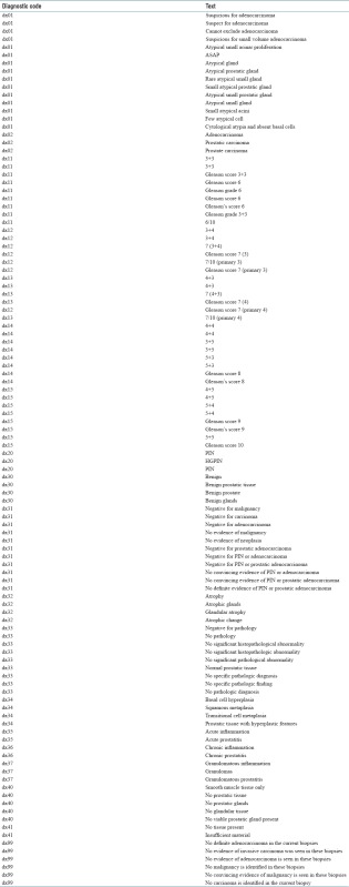
Individual parts were then compared to a dictionary of 110 diagnostic phrases that were matched to 27 diagnostic codes [Appendix 3], using string matching or fuzzy string matching using the open library “google-diff-match-patch” (https://code.google.com/p/google-diff-match-patch/). If the surgical case could not be separated into individual parts, the dictionary of diagnostic phrases was run against the complete (free text) diagnosis.

Subsequent to diagnostic coding, nonsensical concurrent diagnoses were excluded based on a second dictionary that defined a diagnostic hierarchy. The diagnosis of “adenocarcinoma” (not otherwise specified) and “suspicious for adenocarcinoma” typically do not occur within an individual part of a case; however, both “adenocarcinoma” and “suspicious for adenocarcinoma” would be found if the diagnostic line reads “suspicious for adenocarcinoma,” as the one is a substring of the other. In this case, the program assumed “suspicious for adenocarcinoma” and purged the code for “adenocarcinoma”. If a Gleason score was found, it would supersede “adenocarcinoma” not otherwise specified.

Diagnostic codes for a case were compared within a hierarchy to determine the “worst” diagnosis. The hierarchy was as follows: benign (completely negative, no prostatic intraepithelial neoplasia (PIN) or ASAP), high-grade PIN, suspicious for malignancy/atypical small acinar proliferation (ASAP), adenocarcinoma (not graded), adenocarcinoma WHO/ISUP grade (group) 1 (WHO 1), WHO/ISUP grade 2 (WHO 2), WHO/ISUP grade 3 (WHO 3), WHO/ISUP grade 4 (WHO 4), and WHO/ISUP grade 5 (WHO 5). Terms higher in the hierarchy imply that less aggressive pathology can be present, for example, WHO/ISUP grade 3 implies there is no WHO4 or WHO5 but there could be ASAP or WHO2. The “worst” diagnosis was termed the “WHO summary score”.

Reporting at our institutions is partially structured and prostate biopsies (in the later 3 years of the study period) were usually done with a synoptic report that contains a (Method S) Gleason score. The program searched for the prostate biopsy synoptic and (if found) extracted from it the primary Gleason pattern, secondary Gleason pattern, percent tumor, number of positive cores, and total number of cores.

Following diagnostic coding (determination of the “WHO summary score”), the program identified the specimen number, requesting MD, pathologist, number of specimen parts (as per requisition), number of specimen parts found, primary Gleason pattern, secondary Gleason pattern, percent tumor, number of positive cores, and total number of cores, WHO summary score, (requisition provided) clinical history, part list (as per the requisition), and (free text) diagnosis. These data were inspected for trends and then tabulated.

The data were fully anonymized and this included replacing (1) surgical numbers, (2) submitting MD, and (3) pathologist with unique random numbers. The unique random numbers with their nonanonymous/identifiable counterparts were written into a separate “key” file, to allow retrieval of individual cases and identify individual MDs associated with the case, if this should be necessary. The order of the anonymized data was fully randomized by sorting by the column that represents the deidentified surgical number.

The fully anonymized/randomly ordered file was reviewed to assess the coding accuracy of the program; the WHO summary score was compared to the free text diagnosis and Gleason score in the synoptic (if applicable).

The resulting data were used to (1) generate the funnel plots [Figure 1], (2) perform logistic regression analyses, and (3) create the “normalized deviations plots” [Figure 2].

Figure 1.

The “o”s on the plots represents individual pathologists. For each pathologist, one can read off how many cases they interpreted and the diagnostic rate in percent, i.e., the percentage of cases the pathologist called that diagnosis. The pair of dashed lines represents ± two standard errors (95% confidence interval) from the median diagnostic rate. The pair of solid lines represent ± three standard errors (99.8% confidence interval). (a) Negative, (b) PIN, (c) ASAP, (d) WHO 1 (Gleason score 6), (e) WHO 2 (Gleason score 3 + 4), (f) WHO 3 (Gleason score 4 + 3), (g) WHO 4 (Gleason score 8), (h) WHO 5 (Gleason score 9 or 10)

Figure 2.

These plots show the diagnostic rates in relation to the group median (zero). Positive numbers imply a relative over call and negative numbers imply a relative under call. As the numbers are generated by dividing through by the standard error, pathologists that read different numbers of cases can readily be compared. Each plot represents one pathologist. Diagnoses that have a standard error > 2 or <−2 are unlikely due to sampling (P < 0.05). Diagnoses that have a standard error >3 or <−3 are very unlikely (P < 0.001) to be due to sampling alone, and suggest diagnostic bias. (a) Pathologist 4, (b) pathologist 9, (c) pathologist 10, (d) pathologist 11, (e) pathologist 13, (f) pathologist 14, (g) pathologist 17, (h) pathologist 20

The curves in the funnel plots were centered on the median DR and generated using the multiples of the standard error, calculated from the normal approximation of the binomial distribution [Appendix 1].

Clinical completeness was assessed by searching in the clinical history field for the term “Not available on requisition.” “Not available on requisition” is a standard phrase entered at the time of accessioning if the pathology consultation is defective with regard to the clinical history. Clinicians submitting <25 cases were excluded from the analysis.

RESULTS

In the study period (2011–2016), there were 160,322 surgical pathology reports, of which 3,854 were identified as prostate biopsies. Most of the prostate biopsies 92% (3,529) could be separated into individual parts.

A synoptic report was present in 1,640 prostate biopsy cases, and the WHO summary score (based on string matching) compared well with the synoptic report WHO grade [Table 1].

Table 1.

Free text versus synoptic

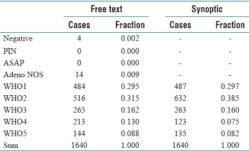
It should be noted that the grading (Method S versus Method H) is not directly comparable for most of the grading categories; however, WHO1 should be the same when grading through the highest grade (Method H) and representative/summary grade (Method S). There is a mismatch in WHO1; however, it is relatively small in relation to the total number of cases [Table 1].

Classification failures were the result of unusual report formatting in most cases. The classification failures were higher in the unparsed reports, and based in part on failures of the parsing algorithm; this is what explains the four “negative” biopsies in Table 1.

Two audits consisting of pathologist (first author, fifth author) interpretations of 400 random reports yielded three categorization errors. A second pathologist (second author) independently audited 300 other reports and found one categorization error.

Twenty-seven pathologists read 40 or more sets of prostate biopsies and together assessed 3,690 cases. 164 cases were read by a total of 13 pathologists; these cases were excluded from the interrater variation analysis as each of those pathologists read <40 cases.

The DRs varied significantly by pathologist [Table 2]; however, agreement tended to be better with cancers than with benign diagnoses.

Table 2.

Diagnostic rates by pathologist

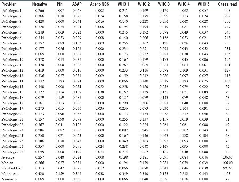
The reports of the significant outliers in the “ASAP” category were examined more closely. It was noted that a number of the reports read “atypical glands, favor benign,” “atypical glands, suggest follow-up” or “atypical glands, pending IHC.” It could be argued that some of these do not fit into a category with “suspicious for malignancy;” however, it is our opinion that they do not really fit well with “benign” either. It is our opinion that this reporting terminology is suboptimal; ideally, a case should be either suspicious or not, and the reporting language should leave no ambiguity.

Logistic regression analyses were done for the individual diagnostic categories and were found to have statistically significant outliers (P < 0.05) for all diagnoses (details not shown). Likewise, funnel plots constructed for each diagnosis showed DRs >2 standard errors from the median DR [Figure 1].

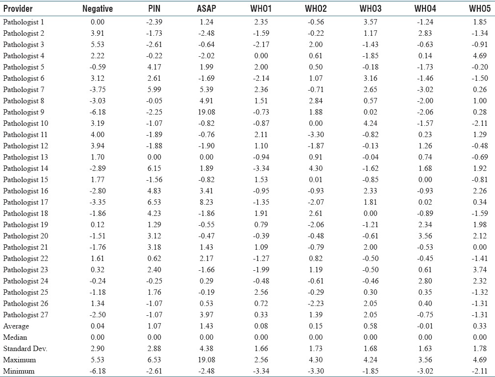
The DR data were normalized by the median rate and the standard error to (1) adjust for the pathologist case volume and (2) allow comparisons between the DRs in one plot for each pathologist [Appendix 2]. The plots generated from the normalized data we refer to as “normalized deviations plots”. They represent the relative over-calls and under-calls of a physician, and typically zigzag in relation to the zero value. Table 3 is a normalized version of Table 2. [Figure 2] shows representative normalized deviation plots.

Table 3.

Normalized deviations from the median in standard errors by pathologist

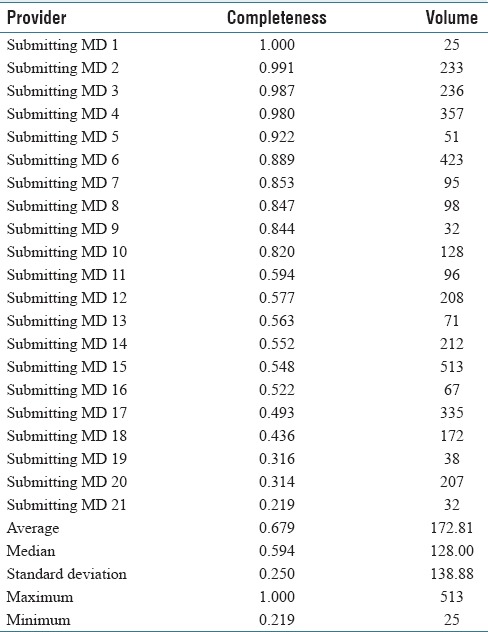
The clinical history completeness was stratified by the submitting physician and the findings are shown in Table 4. Completeness varied from 22% to 100%. Completeness was also stratified by the hospital site; one site had a completeness rate of 54% and the other site a completeness rate of 95%. The relative case volumes of the two institutions are of similar magnitude; thus, there is no doubt that the difference is of statistical significance. It was assumed that everything that is not “Not available on requisition” is an adequate history; however, this is unlikely to be true and represents a best case scenario. The number of cases submitted (volume) appears to have no relationship to the completeness.

Table 4.

Clinical History Completeness

Limitations of the study include (1) the (diagnostic) categorization accuracy of the computer code, and (2) the lack of objective clinical outcome data to compare to the pathological classification.

In the context of the computer classification, it is possible that particular reporting styles are consistently misclassified; thus, a review of the report wording/computer interpretation is important to overcome this limitation. This limitation was partially addressed by casually examining the reports of pathologists that were outliers, tweaking the dictionary of diagnostic terms, and re-running the analysis code dozens of times.

The analysis was restricted to what was found in the original report. Report addenda were extracted from the reports but not analyzed. This is a true limitation, as a number of pathologists signed cases as “pending IHC” or “pending addendum.” We believe this practice should be discouraged, as it may make reports difficult to properly interpret quickly. Further work could include (1) analyzing report addenda and (2) searching for “pending IHC” and similar terms to better understand the prevalence and implications of this reporting style.

A group of pathologists may systematically misclassify cases (i.e., an institutional bias). The techniques in this paper would not identify this bias. Expert review, in conjunction with the techniques presented herein, is important; however, we view expert review as an overvalued surrogate for hard clinical outcome data.

DISCUSSION

DR information in free text reports is accessible with some effort. The relatively good computer categorization accuracy in this study (~1% error) has its basis in (1) the iterative refinement of the dictionary of diagnostic terms, and diagnostic pruning of nonsensical concurrent diagnoses and (2) relative paucity of diagnostic categories in prostate pathology, in comparison to other domains of pathology, such as breast pathology.

The report formatting and reporting style may be modifiable factors that would facilitate more accuracy in the computer categorizations. Reports where diagnoses were lumped could be interpreted in most cases; however, if the parts were out of order or mislabeled (e.g., “A, P, C, D…” instead of “A, B, C, D…” due to a transcription/voice dictation error) the program could not parse it.

The normalized deviations from the median (shown on the normalized deviations plots) provide insight into an individual pathologist's diagnostic bias. All plots had at least one zero crossing, as expected in the context of mutually exclusive (summary) diagnoses that form a complete or near complete set of diagnostic possibilities; the plainly stated corollary is if a pathologist over calls one diagnosis they will under call another one. Considered from the individual pathologist's perspective, it is useful to know not only the over calls but also the associated under calls. For example, if a pathologist over calls ASAP it is likely that they are under calling (1) benign, (2) PIN, or (3) WHO1 cancer, or (4) some combination of the preceding.

The differences in prostate cancer grading between the Method S and Method H, imply there may be a Will Rogers phenomenon associated with the adoption of Method S grading.[5] Cases classified with Method S leads to lower grades in a subset of patients, which in turn would result in more conservative treatments (?undertreatment) in relation to Method H. This issue needs to be examined more closely. The impression of several authors is that the interrelationship between Method S and Method H is rather complex. We suspect that pathologists working in areas where Method H is predominant are aware of the grading implications and more frequently may under call a small amount of higher grade cancer in a case that is otherwise of lower grade. The magnitude of this issue has been elucidated somewhat by Berney et al. and is discussed in various papers including Athanazio et al. and Arias-Stella et al.[6,7,8] It is of interest to us; however, beyond the scope of the current study.

The plots show significant diagnostic variation between pathologists and suggest that there is a diagnostic bias. We believe that once identified, the diagnostic bias can be corrected.

Five pathologists are considered urologic pathologists; one has a formal urologic pathology fellowship while the remaining four have > 10 years of genitourinary experience each. These pathologists were also outliers, and the trend data suggests that the disagreement is not substantially better. This suggests more uniformity/reproducibility is not as simple as “more subspecialization is required.” It is noted that older pathologists tended to call more WHO1. The reasons for this are not completely clear; however, the trend raises the possibility that changes in the Gleason scoring system (first made over a decade ago,[9] and updated in 2014[10,11]) may not have been adopted by some pathologists.

The clinical history completeness shows significant variation between providers and institutions, suggesting institutional culture may be a strong determinant of history completeness. In our jurisdiction providing a clinical history is a legal requirement, however, that does not appear to influence behavior.[12] We believe that history completeness should be tracked as a quality metric, as it is in another jurisdiction In our country, and tracking should be made part of laboratory accreditation.[13]

Funnel plots and normalized deviations plots are tools that allow one to easily identify outliers and understand possible over calls with their associated under calls. A similar analysis can be done with logistic regression, where the interpreting pathologists are used as (categorical) predictor variables for the response variable of DR (analysis not shown); however, we believe this is less accessible to physicians and stakeholders, due to its complexity and does not significantly add to how the data is presented in funnel plots and normalized deviations plots.

With funnel plots, unlike traditional inter-rater variability studies and case reviews, the detectable call rate differences is limited by the number of cases interpreted and can practically be considered the “width” of the funnel– the distance from the upper edge of the funnel to the lower edge of the funnel. The implications of this are (1) the assessment of small case volume practices and rare specimens is limited, and (2) large practices or regional databases can strongly suggest relatively small significant differences that would be resource intensive to obtain through case reviews. An advantage over case reviews is that the comparison is unbiased. In addition, if cases from a population are reviewed by a pathologist that services that population their call rate can be informative when considering diagnostic discrepancies. At the specimen level, the pathologist's rate data have predictive value; however, it is not determinative. If a pathologist has a low call rate for a particular diagnosis (e.g., WHO 5) yet has made that call on a particular case, the probability may be higher that it is confirmed on review. As such funnel plots compliment case reviews and can provide information similar to inter-rater studies. Diagnoses with lower kappa values on inter-rater variability studies (e.g., HGPIN[14]) will tend to have a higher number of outliers when examined with funnel plots.

Funnel plots are similar to control charts. Control charts are widely used in manufacturing engineering to do statistical process control and have found their way into the medical literature, in a series of papers dubbed “next generation quality.”[15,16] Next generation quality is continuous quality improvement using objective clinical data to provide feedback within a formal framework to improve quality. In pathology, the feedback loop, from a process perspective, has been relatively weak; pathologists generally do not know their diagnostic call rates. Changing how we view observational data, seeking it and using it will lead to the next generation in quality.

Observational anatomical pathology data ought to be looked at continuously and is hypothesis generating. Hypotheses (e.g., Pathologist X over calls diagnosis Y) have to be proposed and tested. The outliers may be “right” and this can only be determined by objective review in conjunction with hard objective outcome data. We have started down this path in one of our institutions; an earlier study focused on colorectal polyps prompted us to review a set of polyps with a gastrointestinal pathology expert. Within a few months, we plan to revisit the data, assess for change, and examine whether the reproducibility has increased. In the context of this project, we likewise plan to review findings after accrual of significant additional cases and are actively encouraging pathologists to show cases which they appear to be over- or under-calling on the basis of the analysis herein.

CONCLUSION

The techniques herein compliment traditional inter-rater studies in pathology, and random case reviews.

Looking at the operational data with statistical tools and using it to control processes (statistical process control) is the norm in other industries. Pathologists must seek the data, analyze it, and let it drive change.

The data presented herein suggests that there is room for improvement and more work to do. We hope that the data showing what the practice is now will be seen as sober assessment of the current state without which positive change (better risk stratification, more appropriate treatment, lower costs, and better outcomes) is difficult to achieve.

Financial support and sponsorship

Nil.

Conflicts of interest

There are no conflicts of interest.

APPENDICES: Appendix 1

The funnel plots were constructed based on the following theoretical consideration:

M = i + E + B

Where:

• M = Measured diagnostic rate

• i = Ideal diagnostic rate

• E = Error due to sampling

• B = Bias of the interpreting physician.

If B is assumed to be zero (null hypothesis valid), M estimates i. We chose the median DR of the pathologist group as an estimate of the ideal DR, for example, the ideal WHO1 rate was 0.194 as per Table 2. The median was chosen to avoid bias from significant outliers.

The ideal DR (estimated by the median DR of the pathologist group) was taken to be the center of the funnel.

Pathologists interpreting very few cases have poor estimates of their DR. To limit the randomness of case assignment on the group median rate, pathologists reading few specimens were excluded from the analysis. The limit (>40 cases) was an arbitrary choice.

The funnel lines were calculated using the standard error (SE) of the normal approximation to the binomial distribution:

SE = sqrt (i [1 − i]/n)

Where:

• SE = Standard error estimated using the normal approximation to the binomial distribution

• i = Ideal diagnostic rate (estimated by the median diagnostic rate of the pathologist group)

• n = Number of specimens read by the pathologist.

Example:

• The SE for pathologist 13's WHO1 rate is:

• SE = sqrt (0.194 × (1 − 0.194)/113)

• SE = 0.0372.

Appendix 2

The normalized DR was calculated as follows:

Nj = (Mj − i)/SEj

Where:

• Nj = the normalized DR for pathologist j

• j = the measured DR for pathologist j

• i = ideal DR (estimated by the median DR of the pathologist group)

• SEj = standard error estimated using the normal approximation to the binomial distribution, based on how many specimens pathologist j interpreted [Appendix 1].

Example:

The Nj for pathologist 13's WHO1 rate is:

Nj = (0.159 − 0.194)/0.372.

Nj = −0.94.

Appendix 3: Dictionary of diagnostic phrases and diagnostic codes

REFERENCES

- 1.Bragg F, Cromwell DA, Edozien LC, Gurol-Urganci I, Mahmood TA, Templeton A, et al. Variation in rates of caesarean section among English NHS trusts after accounting for maternal and clinical risk: Cross sectional study. BMJ. 2010;341:c5065. doi: 10.1136/bmj.c5065. [DOI] [PMC free article] [PubMed] [Google Scholar]
- 2.Napolitano G, Marshall A, Hamilton P, Gavin AT. Machine learning classification of surgical pathology reports and chunk recognition for information extraction noise reduction. Artif Intell Med. 2016;70:77–83. doi: 10.1016/j.artmed.2016.06.001. [DOI] [PubMed] [Google Scholar]
- 3.Spiegelhalter DJ. Funnel plots for comparing institutional performance. Stat Med. 2005;24:1185–202. doi: 10.1002/sim.1970. [DOI] [PubMed] [Google Scholar]
- 4.Mayer EK, Bottle A, Rao C, Darzi AW, Athanasiou T. Funnel plots and their emerging application in surgery. Ann Surg. 2009;249:376–83. doi: 10.1097/SLA.0b013e31819a47b1. [DOI] [PubMed] [Google Scholar]
- 5.Albertsen PC, Hanley JA, Barrows GH, Penson DF, Kowalczyk PD, Sanders MM, et al. Prostate cancer and the will rogers phenomenon. J Natl Cancer Inst. 2005;97:1248–53. doi: 10.1093/jnci/dji248. [DOI] [PubMed] [Google Scholar]
- 6.Berney DM, Algaba F, Camparo P, Compérat E, Griffiths D, Kristiansen G, et al. The reasons behind variation in Gleason grading of prostatic biopsies: Areas of agreement and misconception among 266 European pathologists. Histopathology. 2014;64:405–11. doi: 10.1111/his.12284. [DOI] [PubMed] [Google Scholar]
- 7.Athanazio D, Gotto G, Shea-Budgell M, Yilmaz A, Trpkov K. Global Gleason grade groups in prostate cancer: Concordance of biopsy and radical prostatectomy grades and predictors of upgrade and downgrade. Histopathology. 2017;70:1098–106. doi: 10.1111/his.13179. [DOI] [PubMed] [Google Scholar]
- 8.Arias-Stella JA, 3rd, Shah AB, Montoya-Cerrillo D, Williamson SR, Gupta NS. Prostate biopsy and radical prostatectomy Gleason score correlation in heterogenous tumors: Proposal for a composite Gleason score. Am J Surg Pathol. 2015;39:1213–8. doi: 10.1097/PAS.0000000000000499. [DOI] [PubMed] [Google Scholar]
- 9.Epstein JI, Allsbrook WC, Jr, Amin MB, Egevad LL. ISUP Grading Committee. The 2005 International Society of Urological Pathology (ISUP) consensus conference on Gleason grading of prostatic carcinoma. Am J Surg Pathol. 2005;29:1228–42. doi: 10.1097/01.pas.0000173646.99337.b1. [DOI] [PubMed] [Google Scholar]
- 10.Egevad L, Delahunt B, Srigley JR, Samaratunga H. International Society of Urological Pathology (ISUP) grading of prostate cancer _ An ISUP consensus on contemporary grading. APMIS. 2016;124:433–5. doi: 10.1111/apm.12533. [DOI] [PubMed] [Google Scholar]
- 11.Epstein JI, Egevad L, Amin MB, Delahunt B, Srigley JR, Humphrey PA, et al. The 2014 International Society of Urological Pathology (ISUP) consensus conference on Gleason grading of prostatic carcinoma: Definition of grading patterns and proposal for a new grading system. Am J Surg Pathol. 2016;40:244–52. doi: 10.1097/PAS.0000000000000530. [DOI] [PubMed] [Google Scholar]
- 12.Public Hospitals Act, R.R.O. 1990, Regulation 965, Hospital Management [Internet]. Government of Ontario, Laws and Regulations. [Last accessed on 2016 Dec 20; Last cited on 2017 Apr 28]. Available from: www.ontario.ca/laws/regulation/900965#BK23 .
- 13.Duggan MA, Trotter T. Alberta Health Services: Anatomical Pathology Quality Assurance Plan. Canadian Journal of Pathology. 2016;8:10–35. [Google Scholar]
- 14.Giunchi F, Jordahl K, Bollito E, Colecchia M, Patriarca C, D’Errico A, et al. Interpathologist concordance in the histological diagnosis of focal prostatic atrophy lesions, acute and chronic prostatitis, PIN, and prostate cancer. Virchows Arch. 2017;470:711–5. doi: 10.1007/s00428-017-2123-1. [DOI] [PubMed] [Google Scholar]
- 15.Luttman RJ. Next generation quality, part 1: Gateway to clinical process excellence. Top Health Inf Manage. 1998;19:12–21. [PubMed] [Google Scholar]
- 16.Luttman RJ. Next generation quality, Part 2: Balanced scorecards and organizational improvement. Top Health Inf Manage. 1998;19:22–9. [PubMed] [Google Scholar]