

Abstract
Magnet-tipped, elastic rods can be steered by an external magnetic field to perform surgical tasks. Such rods could be useful for a range of new medical applications because they do not require either pull wires or other bulky mechanisms that are problematic in small anatomical regions. However, current magnetic rod steering systems are large and expensive. Here, we describe a method to guide a rod using a robot-manipulated magnet located near a patient. We solve for rod deflections by combining permanent-magnet models with a Kirchhoff elastic rod model and use a resolved-rate approach to compute trajectories. Experiments show that three-dimensional trajectories can be executed accurately without feedback and that the system’s redundancy can be exploited to avoid obstacles.
Index Terms: Catheter, magnetic guidance, minimally invasive surgery, redundant robots
I. Introduction
Needles, catheters, and other rod-shaped instruments are difficult to steer by hand. Pull wires and other internal steering mechanisms can help guide rods to targets [1], [2], but usually require a widened rod diameter. One alternative is to apply magnetic fields to deflect a rod that has a permanent magnet attached near its tip [3], [4]. Use of magnetic fields for rod steering does not require steering mechanisms along the length of a rod and may, thus, facilitate construction of very thin, yet steerable rods.
Three commercial systems currently use magnetic fields to guide cardiac catheters. Stereotaxis corporation’s Niobe ES system uses a pair of large, neodymium-iron-boron (NdFeB) magnets to create a magnetic field across an operating table [5]. The pair of magnets are robotically positioned to guide a magnet-tipped catheter within the heart. The Catheter Guidance Control and Imaging [6] system and the Aeon Phocus [7] both use solenoid arrays that surround the patient and create an adjustable field to guide cardiac catheters. Similar to the Niobe ES system, both systems are large and immobile, require dedicated floor space, and restrict access to a patient. However, the large-scale of these systems is necessary for manipulating cardiac catheters, which have relatively wide diameters of 2–4 mm [6].
Miniature rods may be beneficial for dexterous manipulation in the many small cavities of the body, such as the eye, ear, spine, skull base, or lungs. For example, Clark et al. [8] proposed guiding a magnet-tipped implant electrode through the cochlea, and Ullrich et al. [9] proposed guiding a magnet-tipped microcatheter within the eye. The very large commercial magnetic steering systems may not be economical for miniaturized applications, where less powerful magnetic fields may suffice to do useful work. MRI scanners have been investigated for steering solenoid-tipped rods [10]–[12]; however, most procedures are not performed in an MRI scanner because of either hospital workflow or cost considerations.
A single permanent magnet can serve as a compact and inexpensive magnetic field source for steering rods. Clark et al. [8] proposed using a robot-manipulated magnet to guide a cochlear implant electrode. Planar bending was considered exclusively, which required only one rotation and one translation of the external magnet. Mahoney and Abbott [13] described steering a magnetic capsule in three-dimensional (3-D) space by robotically manipulating a permanent magnet, but the capsule was untethered.
Tunay [14], of Stereotaxis corporation, presented a method to guide a magnet-tipped rod in a two-dimensional plane, using feedback from an electromagnetic localization system. Later, Tunay used Cosserat rod theory to model the 3-D static deflection of a magnet-tipped catheter and simulated rotations of a uniform magnetic field to guide a catheter around an obstacle, but continuous tip trajectory control was not demonstrated in the simulation [15], [16]. Greigarn and Çavoşoğlu [12] presented a motion planning algorithm for a solenoid-embedded catheter modeled as a chain of rigid links connected by springs, and showed with simulations that the method required feedback to compensate for drift.
This paper addresses the previously unsolved problem of guiding a magnet-tipped rod along arbitrary, 3-D trajectories, using a single, robot-manipulated magnet. We consider a rod deployed by an advancer, which can insert and possibly rotate the rod axially. We relate the motions of the advancer and robot to deflections of the rod tip using a Kirchhoff rod model, and invert this model using a resolved-rate approach to follow trajectories.
We envision our method to be an inexpensive solution for steering miniature rods. Our method does not consider position feedback, which is difficult to obtain for miniature rods, but does not preclude future extension to include feedback.
For conciseness, we will refer to the range of magnet-tipped elastic devices simply as “rods” in the remainder of this paper, but our methods apply to narrow elastic rods with any cross-sectional profile, including solid rods and tubular cannulas.
II. Magnet-Tipped Rod Model
We use the Kirchhoff rod model [17]–[21] to solve for large, 3D deflections of a magnet-tipped rod. A large deflection model is appropriate for surgical tasks because linearized models typically assume deflections on the order of a rod’s thickness. The Kirchhoff model represents a rod as a one-dimensional curve that can bend and twist under load, but is assumed to be inextensible and unshearable.1 The static Kirchhoff rod problem culminates in a set of ordinary differential equations. After reviewing this problem using the notation presented in [22], we will solve for rod deflections as solutions to a two-point boundary value problem (BVP).
A. Kinematics
The centerline of an undeflected rod is represented by an arc-length parameterized space curve , expressed in some fixed frame. An orthonormal frame is attached to each point on , and is represented by a rotation matrix , where the tilde symbol denotes association with the undeflected curve. Each local coordinate frame represents the orientation of rod material at the point where it is attached. Under load, deflects to a curve p(s), and rotate to R(s), in general. Fig. 1 illustrates the deflection of a rod and the ensuing rotations of a few local frames.
Fig. 1.
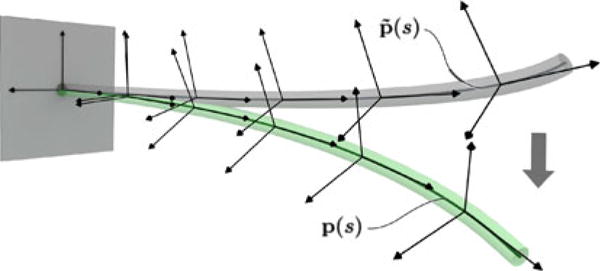
Rod modeled in Kirchhoff’s theory as a space curve with a local coordinate frame attached to each point. A few frames are shown at corresponding positions on an undeflected curve (which may be arbitrarily precurved) and on the deflected curve p(s) of the same rod.
We assign frames on the undeflected curve such that the z-axis of each frame is tangent to the curve. Frames constrained this way are called adapted frames. An arc-length parameterized curve has a tangent vector of unit length [23, Ch. 2]. Using a prime symbol to denote differentiation with respect to s, the adapted frame constraint can be written as
| (1) |
in which .
The angle of rotation of each frame about a rod’s centerline is not constrained by (1), and must be chosen in some way. If the rod is initially straight and has a radially symmetric cross-section, then choosing all as identity matrices aligns them to the fixed frame. If the rod is precurved and has asymmetric cross-sections, then the x and y axes of each frame can be aligned to the principle axes of each cross-section. If the rod is precurved and radially symmetric, then any of several curve framing methods based on the geometry of the centerline can be used to assign adapted frames, such as the Frenet–Serret formulas [23, Ch. 2] or the parallel transport method [24].
B. Constitutive Relations
The derivative of R(s) with respect to arc-length can be expressed as
| (2) |
in which U is a skew-symmetric matrix. Omitting the argument s for brevity
| (3) |
The elements ux, uy, and uz can be seen as components of an axial vector u. Curvatures about the x and y axes are given by ux and uy, respectively, and the torsional twist rate is denoted by uz. A vector is found in a similar fashion from . Vectors can also be mapped to skew-symmetric matrices, an operation we will denote by [•] ×.
The vector gives the strain at each material point s. The bending strains about the local x and y axes are given by Δux (s) and Δuy (s), respectively, and the torsional strain is given by Δuz(s).
We will assume that the rod material is linear-elastic with modulus E(s) and shear modulus G(s). The second moments of area about the principle axes of the rod cross-section are denoted by Ix (s) and Iy (s), and polar moment of inertia about the rod’s centerline is denoted by Jz (s). Omitting the argument s, these variables can be arranged into a diagonal matrix
| (4) |
The internal moment at any point is proportional to the internal strains. This constitutive relationship can be written as
| (5) |
It is useful to rearrange the above-mentioned equation in the form
| (6) |
which gives terms of matrix U in (2).
C. Equilibrium Equations
We show the forces and torques acting on an isolated segment of a rod in Fig. 2. The segment extends from an arbitrary point p(s) to the tip p(L). The internal force n(s) and internal torque τ(s) act in a positive sense across the cut on the portion of the rod that extends from the base of the rod to s.
Fig. 2.
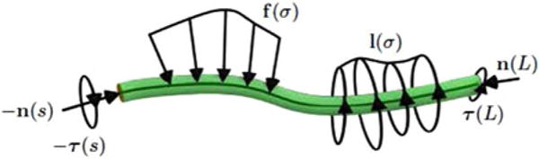
Equilibrium equations are found by cutting the rod at an arbitrary point p(s) and summing all loads from this point to the rod tip. All loads act on the rod’s centerline and include an internal force and torque at s (n(s), τ (s)), distributed forces and torques along the segment (f (σ), l(σ)), and a force and torque at the tip (n(L), τ(L)).
Distributed forces and torques that act along the rod are denoted by f (σ) and l(σ), respectively, where σ is a dummy variable for integration. Such loads could be caused by tissue in contact with the rod, for example. The sum of forces on the cut segment of the rod is
| (7) |
The total moment on the segment, taken about the origin of the fixed frame, includes the internal torque at p(s), the moment of the internal force at p(s), the integral of the distributed torque, the integral of the moment of the distributed forces, the tip torque, and the moment of the tip force
| (8) |
Equilibrium differential equations are found by differentiating (7) and (8) with respect to s to obtain
| (9) |
| (10) |
D. Boundary Conditions
The advancer, robot, and external magnet enter our model through boundary conditions, which we will specify for rods both with and without a protective bushing, shown schematically in Figs. 3 and 4. In both configurations, a rigid post connects the base of the rod to actuators inside the advancer, which are not shown.
Fig. 3.
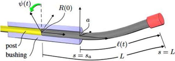
Bushing, shown in section view, guides the rod to the operative region. The base of the rod is actuated via a rigid post that translates the rod by a distance ℓ(t) and rotates it by an angle ψ(t) relative to frame a. A two-point boundary value problem is solved with endpoints at sa and L.
Fig. 4.
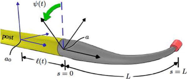
Bushing may be discarded to accommodate either tapered or other unusual rod shapes. In this case, the BVP is solved over the fixed interval [0, L] and the advancer displacements ℓ(t) and ψ(t) are interpreted as parameters of a rigid transformation of frame a with respect to an initial pose a0.
The bushing is useful as a rigid conduit to guide a rod to an operative region. A fixed frame, labeled a in Fig. 3, is placed at the distal end of the bushing, oriented such that its z-axis is aligned with the bushing’s centerline. The advancer translates the rod by a distance ℓ(t) along the z-axis and rotates it by an angle ψ(t) about the same axis (such rotation may be useful either with a precurved rod or if the tip magnet axis is not aligned with the rod centerline). The time t is held constant when solving the BVP and will be omitted as an argument in the remainder of this section. We will view the advancer and robot joints as functions of time in Section III, where the rod’s motion is planned as a succession of equilibrium states.
The material point that coincides with the origin of frame a is denoted by sa = L − ℓ, where L is the total length of the rod. We will solve the BVP over the interval [sa, L], which spans the unconstrained part of the rod.
If the rod is radially symmetric, then it may twist within the bushing. We assume that the bushing is frictionless, and therefore, cannot apply torque about the rod centerline. If the rod is precurved, then the bushing exerts reaction forces to conform the rod to the bushing’s centerline, but these transverse forces cannot cause torsional deformation because the shear center of a Kirchhoff rod coincides with its centerline [25]. Thus, deformation in the bushing consists solely of twisting around the local z-axis, and is caused exclusively by τz (sa), the z-component of the internal moment at the distal end of the bushing. The z-axes of the local frames are aligned within the bushing; thus, the transposed rotation matrix in (6) does not affect the z-component of u(s), which becomes
| (11) |
The bushing constrains the position and direction of the rod centerline at p(sa), but the frame R(sa) is rotated about the z-axis by an angle
| (12) |
Thus, the boundary conditions at sa are
| (13) |
| (14) |
where Rz (·) is a rotation about the fixed z-axis. Note that the angle ϕ depends on the constant τz (sa), which is unknown at the outset of solving the BVP.
If a nonradially symmetric rod is used, then a bushing may be designed to prevent the rod from either twisting or rotating (e.g., a “D”-shaped rod in a similarly shaped hole). For such a bushing, rotation by ψ could be implemented as rotation of the entire bushing about the fixed z-axis, whereby conditions (13) and (14) can be applied by setting ϕ = ψ.
The pose of the external magnet (frame m) is known, in general, with respect to the robot base frame r from a forward kinematic function in the form
| (15) |
in which T is a 4 × 4 homogeneous transformation matrix, and θ is a joint displacement vector. The field B of the external magnet is assumed available from a field model. We also assume that the pose of the advancer frame a is known relative to the robot base frame r as a transformation . Thus, the field B can be found at position p(L) from coordinate transformations. However, the tip position p(L) depends on the equilibrium solution of the rod, and similar to τz (sa), this constant is an unknown.
It may sometimes be desirable to dispose of the bushing, as shown in Fig. 4. This configuration could be useful if the rod is tapered, for example. We embed frame a in the base of the rod in this case, and interpret ℓ and ψ as displacements of frame a relative to a reference pose at which Tar has been measured. Denoting the displaced position of frame a by a′, the pose of the advancer relative to the magnet now becomes
| (16) |
By setting sa = 0, boundary conditions (13) and (14) hold as stated above.
Next, we consider loads on the tip. The tip magnet may be attached in any orientation with respect to the tip frame R(L), although it may often be convenient to align its magnetization vector with the rod centerline. Let the unit vector in frame R(L) denote the direction of the magnetization vector with respect to the rod tip. The magnetization vector m can be factored as , and is a unit vector expressed in the fixed frame as
| (17) |
The vector depends on the equilibrium tip frame orientation R(L), and in addition to τz (sa) and p(L), must be found when solving the BVP. The numerical method we use to find these variables is described in Section IV-C.
The force and torque applied by the external magnet to the rod tip magnet are found by modeling the tip magnet as a point dipole, and are given by
| (18) |
| (19) |
where B is the field established by the external magnet and G is a gravitational force acting on the tip magnet. The gravitational force acting along the rod may be included as a distributed force f (s) in (10).
The deflected shape of the rod is found by solving (1), (2), (9), and (10), together with the boundary conditions given by (13), (14), (18), and (19).
III. Trajectory Following
A. Forward Kinematics
For trajectory planning, we limit our attention to the solution for the rod tip, and use the variable r(t) to represent the tip pose found by solving the BVP for boundary conditions applied at time t. In general, the components of r(t) may include the tip position p(L) and a parameterization of the tip orientation R(L). The dimension of r(t), which we will denote by d, is either six or more, depending on whether a minimal or other representation of orientation is used. However, attachments to the rod tip will often be axially symmetric, in which case only the tip direction vector will be of interest, and d is equal to five. In practice, the dimension of d may be further reduced to minimize the number of constraints on motion planning, e.g., controlling either the Cartesian rod position or direction only.
The advancer and robot joint variables are combined as
| (20) |
Let p denote the advancer degrees of freedom (DOF), such that p = 1 if only ℓ(t) is actuated, and p = 2 if ψ(t) is also actuated. Thus, if the robot has j joints, then q has dimension p + j.
With the variable q, the forward kinematics of the cooperative advancer-robot system can be expressed as a function
| (21) |
We wish to invert Ω to find a joint trajectory q(t) corresponding to some desired tip trajectory r(t). However, Ω is not amenable to direct inversion because q may not be unique and Ω is found as a solution of a differential equation. We will find solutions to the inverse problem that use the numerically computed geometric jacobian matrix to map the control vector velocity of robot joints to the rod tip spatial velocity
| (22) |
If J is square and full rank, then it can be inverted to solve for a unique . If p + j > d, then the system is redundant to the tip control task, provided that J is full (row) rank. The advancer and robot form a cooperative system in which the rod tip pose is the output, and the robot end-effector is analogous to an intermediate link in a more traditional robot structure, which may be exploited to fulfill various secondary goals. There are typically multiple solutions for the external magnet pose. The Jacobian that maps the spatial velocity of the external magnet to the force/torque wrench on the tip magnet is rank five for dipole magnets [13] (rotations about the dipole axis leave the field unchanged). Thus, perturbations of the external magnet pose alter the tip boundary conditions and change the shape of the rod.
In some cases, we may not have control authority to command arbitrary positions and orientations of the tip. Considering potential applications ranging from ablation to imaging, we believe that achieving the desired position should be prioritized, and only then should the error in the orientation be minimized. There exists a variety of constrained-optimization (nonlinear programming) algorithms that enable (22) to be solved accordingly.
IV. Experimental Methods
We assembled a magnet-tipped rod guidance system to execute trajectories for the rod tip position (d = 3). The experimental apparatus was arranged on a benchtop as illustrated in Fig. 5.
Fig. 5.
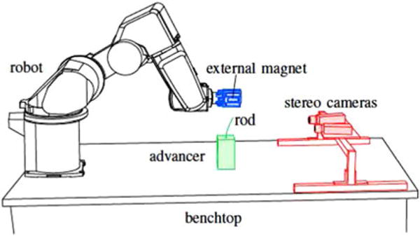
Experimental apparatus. An NdFeB magnet was mounted to a six- degree-of-freedom (6-DOF) serial robot to guide a magnet-tipped rod along trajectories. The length of rod was varied by a 1-DOF advancer. A stereocamera pair was used to measure rod tip positions. The cameras were not used for feedback.
A. Advancer and Magnet-Tipped Rod
The rod was a straight, glass optical fiber (Item 57062, Edmund Optics, NY, USA), 10 cm in length with a diameter of 0.24 mm. Two NdFeB magnets (Cyl-0010, Engineered Concepts, Birmingham, AL, USA) were attached coaxially to the tip of the rod using cyanoacrylate adhesive (Loctite 4014 Prism Instant Adhesive, Henkel Corp., Rocky Hill, CT, USA). The magnets were cylinders, each 0.75 mm in diameter and 1 mm long. Each magnet was grade N50, and was magnetized along its cylindrical axis.
The advancer, shown in Fig. 6, consisted of a rigid acrylic frame that housed a piezoelectric linear motor (SLC-1770, SmarAct GmbH, Oldenburg, Germany) which had an encoder resolution of 1 μm. The rod was attached to a vee-shaped clamp on the moving slide of the motor. This clamp applied the boundary conditions stated in (13) and (14), with ψ = 0, as we did not rotate the rod. A low-friction bushing on the top surface of the acrylic was fabricated from a 3.2 mm thick sheet of an acetal polymer using a CO2 laser cutting machine.
Fig. 6.
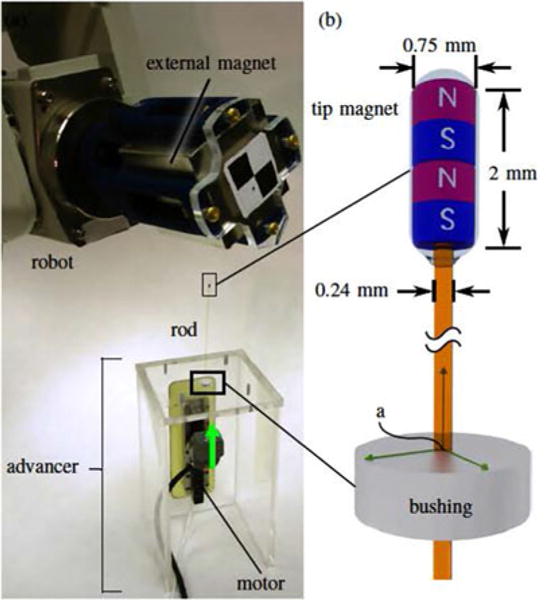
(a) Cube-shaped NdFeB magnet, with an edge length of 5.08 cm, was held in a fixture attached to the robot. (b) The rod was an optical fiber with two NdFeB magnets attached to its tip. It was pushed by a linear motor through a bushing that constrained the position and direction of the rod.
B. Robot and External Magnet
A 6-DOF serial robot (Model RV-3S, Mitsubishi Electric US, Inc., Cypress, California) was used to manipulate the external magnet. The robot’s position repeatability was 0.02 mm.
The external magnet was a cube-shaped, grade N52 NdFeB magnet (NB064-N52, Applied Magnets, Plano, TX, USA), with an edge length of 5.08 cm. The magnet was placed in a fixture attached to the robot end-effector, which is shown in Fig. 6. The magnet was oriented in the fixture with its magnetization vector orthogonal to the robot’s sixth joint axis. We modeled the field of this magnet using the exact, closed-form solution for a cuboid magnet derived by Furlani [26, Ch. 4].
C. Trajectory Computation and Control
We planned trajectories using MATLAB software by numerically integrating (22) using the central difference method to approximate the Jacobian from evaluations of (21). Numerical drift was compensated for using the closed-loop inverse kinematics algorithm [27].
We included the gravitational force on the tip magnet, but neglected the distributed force of gravity along the thin rod to speed and simplify computations.
We used the MATLAB function bvp5c by Kierzenka and Shampine [28] to solve the BVP. This function can solve BVPs that include unknown parameters under the boundary conditions, which in our formulation included τz (sa), p(L), and , as explained in Section II-D. Computation of a single rod solution took between 20 and 50 s.
A program was written in the C programming language to control the serial robot and advancer, and to trigger acquisition of stereo images. The program executed preplanned trajectories on a desktop computer with a 2.67 GHz Intel Xeon processor, which ran a Linux Ubuntu 11.04 operating system.
D. Stereo Camera Measurements
Two digital cameras (XCD-X710, Sony Corporation, Japan) were mounted in a stereo configuration to a rigid aluminum frame attached to the benchtop, approximately 40 cm from the advancer. Prior to acquiring experimental images, we used the OpenCV library [29] to find stereo calibration parameters from images of a checkerboard pattern. During trajectory execution, the control software automatically triggered acquisition of image pairs. Each image measured 1024 × 768 pixels, and was processed to correct lens distortion using OpenCV.
To measure a 3-D point, image coordinates of the point were manually selected in corresponding images. The 3-D point was then triangulated using an iterative least-squares method that minimized the stereo reprojection error [30].
E. Calibration
We chose a small set of sensitive parameters, listed in Table I, to calibrate the model. Parameter EIx is the bending stiffness of the rod. The rod had a circular cross-section; therefore, EIy = EIx. The torsional stiffness GJz was calculated to be 5.33 × 10⁻⁶ N m2 from the calibrated value of EIx. The magnetizations of the external magnet Mext and tip magnet Mtip have a large effect on accuracy because the calculated forces and torques on the tip magnet depend on the magnitudes of these two quantities. The mass of the tip magnet mtip determines the gravitational force G in (18). The total rod length L was initially measured to be 10 cm, but the process of manually clamping the rod to the motor caused some uncertainty in this parameter. Parameters δx, δy, and δz are small corrections to the translational components of . Rotational components of were excluded because frame a was defined to be parallel to r in the registration process described above, and enabling rotation between these frames did not significantly improve calibration results during initial sensitivity tests.
TABLE I.
Calibrated Values of Model Parameters
| Parameter | Value |
|---|---|
| EIx | 6.17 × 10⁻⁶ Nm2 |
| ||Mext|| | 1.21 × 10⁶ A/m |
| ||Mtip|| | 1.24 × 10⁶ A/m |
| mtip | 3.65 × 10⁻⁵ kg |
| L | 98.75 mm |
| δx | 2.00 mm |
| δy | 0.43 mm |
| δz | 1 × 10⁻⁵ mm |
A set of 60 randomized q vectors were used for parameter calibration. They prescribed poses for the robot and advancer at which images were acquired with the stereo cameras. The kth rod tip position as measured from the stereo images is denoted by rk. The kth rod tip position found by solving the BVP with controls qk and parameter vector γ is denoted by Ω (qk; γ). An initial guess for γ was selected by coarse adjustment of nominal values. We used the fmincon function in MATLAB to find the parameters γcal that minimize the objective function
| (23) |
This function computes the error between predicted and measured tip positions, summed over the calibration set. We define the tip error as the Euclidean norm of the difference between a measured tip position and a modeled tip position. After finding optimal calibration parameters, the mean tip error for the calibration set was 0.62 mm.
V. Experiments
We guided a rod tip along several 3-D trajectories using the methods of Section III. These trajectories were executed without feedback. The mean and standard deviation (SD) of tip error measurements for each trajectory are presented in Table II, which also lists the number n of tip measurements for each trajectory. Advancer frame coordinate axes are shown in Figs. 7–9, where the positive x-axis points toward the midpoint of the stereo cameras. With the exception of the trefoil knot trajectory discussed below, we planned trajectories using all six joints of the robot. The pseudoinverse of J was used to plan all trajectories except the virtual wall trajectory, in which a weighted generalized inverse was used. For all trajectories, the origin of the external magnet began at point 12 cm directly above the origin of the advancer frame.
TABLE II.
Rod Tip Error
| Trajectory | Mean (mm) | SD (mm) | n |
|---|---|---|---|
| Square, xy plane | 0.98 | 0.22 | 199 |
| Square, zx plane | 0.83 | 0.07 | 199 |
| Square, zy plane | 0.96 | 0.25 | 199 |
| Square, xy plane with obstacle | 1.07 | 0.23 | 249 |
| Trefoil knot, 2-DOF robot | 1.52 | 0.48 | 249 |
Fig. 7.
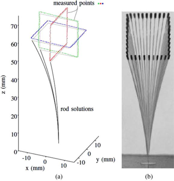
(a) Tip of the rod was guided along three square trajectories, each with an edge length of 2 cm. Measured tip positions are shown as dots, with the planned trajectories shown as solid lines next to the dots. Examples of rod solutions are shown at the starting point of each trajectory. (b) Composite photograph constructed from 40 sampled positions of the zy-plane square trajectory.
Fig. 9.
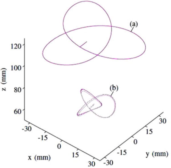
(a) To simulate a 2-DOF robot, the external magnet trajectory was restricted to translations within a plane. (b) The rod tip was guided along a trefoil knot trajectory, a 3-D space curve.
Fig. 7(a) shows tip measurements from three square tip trajectories within mutually orthogonal planes. This experiment tested the ability to track straight lines in various positions and orientations. Each square had a planned edge length of 2 cm, and was executed with a tip velocity of 0.4 mm/s. The center of each square was located 6 cm above the origin of the advancer frame. The full rod shape found by solving the BVP (i.e., the planned shape) is shown at the starting point of each trajectory. A composite photograph of 40 sampled positions from a video recording of the zy-plane trajectory is shown in Fig. 7(b).
We explained how the system’s redundancy could be exploited in Section III. To test this, we projected a virtual planar wall into the robot’s workspace, as shown in Fig. 8. Such a wall could be used to prevent the external magnet from colliding with either the patient or other forbidden region. An artificial potential field was established on the wall, using Khatib’s method [31]. The magnitude of this field increases when approaching the wall. Components of the field’s gradient were used to adjust weights of a weighted generalized inverse solution [32] to (22) so as to deflect the external magnet’s trajectory away from the wall while obtaining the desired tip magnet positions. Use of the gradient of an objective function to adjust generalized inverse weights is described in [33].
Fig. 8.
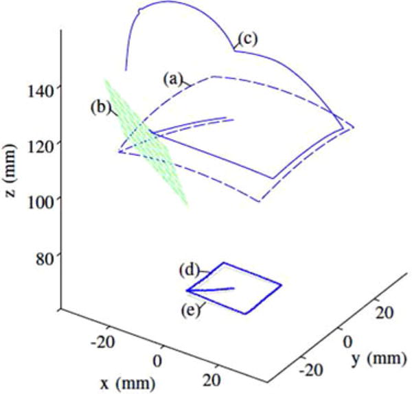
External magnet trajectory (a) violates a virtual wall (b) when used to guide the rod tip along a square trajectory. By using an artificial potential function emanating from the wall to adjust a weighted Jacobian, the external magnet instead moved along trajectory (c). The measured tip positions (d) are shown for external magnet trajectory (c), with the planned trajectory shown as a solid line (e).
The tip trajectory executed with the wall present was a square in the xy plane, identical to that shown in Fig. 7, but now starting from the center of the square and following a diagonal line toward the first corner. Fig. 8 shows both the rod tip measurements and the planned motion of the external magnet centroid, which begins by tracking the diagonal line of the rod tip, but is deflected by the virtual wall. An external magnet trajectory planned without wall avoidance is also shown as a dashed line, and violates the wall (the rod tip measurements for this unweighted external magnet trajectory are those shown in Fig. 7).
Although we believe that it will be useful to build some redundancy into a magnetic steering system similar to the one we describe in this paper, inspection of (21) suggests that a simple, 2-DOF robot can be used to manipulate the external magnet (the advancer provides a third DOF when enabled to translate). For example, the external magnet could either be translated within a plane or gimbaled to rotate about two orthogonal axes.
To explore this, we planned a trajectory for a 2-DOF virtual robot restricted to translate the external magnet in a plane parallel to the xy- plane of the advancer frame, at a height of 12 cm above the origin of the advancer frame. The virtual robot was implemented by restricting our 6-DOF robot end-effector to planar motion. The tip trajectory was a trefoil knot space curve. As shown in Fig. 9, this 3-D tip trajectory was executed using only planar motion of the external magnet.
VI. Discussion
The results suggest that open-loop trajectory following can be sufficiently accurate for some clinical applications, such as steering a miniature, rod-mounted video camera, or guiding a catheter to deliver drugs directly to a tumor. However, clinical application of the methods presented here to a particular procedure will require design and validation of a complete surgical system. Characterization of task-specific rod workspace and accuracy requirements will likely be necessary, as will demonstration that the system’s hardware will be compatible with either medical-imaging equipment or surgical instruments used in the procedure.
For applications either requiring submillimetric accuracy or requiring real-time compensation for tissue motion or tissue–rod interaction forces, the open-loop method could be augmented with feedback from either an external medical imaging system, such as a computed tomography scanner or an ultrasound machine, or from sensors within the rod. The robot’s pose could be adjusted to compensate for sensed disturbances of the rod, but further work is needed to demonstrate closed-loop control in real time.
We solved the rod equations using mainly an interpreted programming language (MATLAB) and adjusted the solver to maximize accuracy, not speed. solution times could be accelerated by fully reimplementing the code in a compiled language such as C++.
The magnitude of rod deflections depends on the distance between the external magnet and the rod tip magnet and the strengths of both. Larger rod deflections (or a larger distance between the external magnet and the rod tip) could be attained by using larger magnets, a less stiff rod, or a longer rod.
VII. Conclusion
Complex, 3-D tip trajectories of magnet-tipped rods are attainable without feedback by robotically manipulating a single permanent magnet. We presented a trajectory planning method that combined a Kirchhoff rod model, a magnetic field model, and the kinematics of a robot and advancer. We linearized this model by computing its Jacobian, and demonstrated accurate trajectory following and obstacle avoidance using resolved-rate motion control.
Acknowledgments
The authors would like to thank Neal P. Dillon, Hunter B. Gilbert, and Richard J. Hendrick for their helpful comments and support. The content of this paper is solely the responsibility of the authors and does not necessarily represent the official views of the National science Foundation or the National Institutes of Health.
This paper was recommended for publication by Associate Editor R. S. Dahiya and Editor P. Dupont upon evaluation of the reviewers’ comments. This work was supported in part by the National Science Foundation under Grant IIS-1054331 and in part by the National Institutes of Health under Grant R01 DC012593 and Grant R01 DC013168 from the National Institute on Deafness and Other Communication Disorders.
Footnotes
Color versions of one or more of the figures in this paper are available online at http://ieeexplore.ieee.org.
These are reasonable assumptions provided that the rod is neither bent into sharp corners nor subjected to extreme lateral loads [21, Ch. 3, Sec. 7].
Contributor Information
Louis B. Kratchman, Department of Mechanical Engineering, Vanderbilt University, Nashville, TN 37235 USA
Trevor L. Bruns, Department of Mechanical Engineering, Vanderbilt University, Nashville, TN 37235 USA
Jake J. Abbott, Department of Mechanical Engineering, University of Utah, Salt Lake City, UT 84112 USA.
Robert J. Webster, III, Department of Mechanical Engineering, Vanderbilt University, Nashville, TN 37235 USA, robert.
References
- 1.van de Berg NJ, van Gerwen DJ, Dankelman J, van den Dobbelsteen JJ. Design choices in needle steering—A review. IEEE/ASME Trans Mechatronics. 2015 Oct;20(5):2172–2183. [Google Scholar]
- 2.Fu Y, Liu H, Huang W, Wang S, Liang Z. Steerable catheters in minimally invasive vascular surgery. Int J Med Robot Comput Assisted Surg. 2009;5(4):381–391. doi: 10.1002/rcs.282. [DOI] [PubMed] [Google Scholar]
- 3.Driller J, Casarella W, Asch T, Hilal SK. The pod bronchial catheter and associated biopsy wire. Med Biol Eng. 1970;8(1):15–18. doi: 10.1007/BF02551744. [DOI] [PubMed] [Google Scholar]
- 4.Driller J, Frei EH. A review of medical applications of magnet attraction and detection. J Med Eng Technol. 1987;11(6):271277. doi: 10.3109/03091908709030141. [DOI] [PubMed] [Google Scholar]
- 5.Carpi F, Pappone C. Stereotaxis niobe magnetic navigation system for endocardial catheter ablation and gastrointestinal capsule endoscopy. Expert Rev Med Devices. 2009;6(5):487–498. doi: 10.1586/erd.09.32. [DOI] [PubMed] [Google Scholar]
- 6.Nguyen BL, Merino JL, Gang ES. Remote navigation for ablation procedures—A new step forward in the treatment of cardiac arrhythmias. Eur Cardiology. 2010;6(3):50–56. [Google Scholar]
- 7.Aeon scientific [Online] Available: http://www.aeon-scientific.com.
- 8.Clark JR, Leon L, Warren FM, Abbott JJ. Magnetic guidance of cochlear implants: Proof-of-concept and initial feasibility study. J Med Devices. 2012 Aug;6(3):035002–035002. [Google Scholar]
- 9.Ullrich F, Schuerle S, Pieters R, Dishy A, Michels S, Nelson BJ. Automated capsulorhexis based on a hybrid magnetic-mechanical actuation system. Proc 2014 IEEE Int Conf Robot Autom. 2014:4387–4392. [Google Scholar]
- 10.Roberts T, Hassenzahl W, Hetts S, Arenson R. Remote control of catheter tip deflection: An opportunity for interventional MRI. Magn Reson Med. 2002;48(6):1091–1095. doi: 10.1002/mrm.10325. [DOI] [PubMed] [Google Scholar]
- 11.Settecase F, et al. Magnetically-assisted remote control (MARC) steering of endovascular catheters for interventional MRI: A model for deflection and design implications. Med Phys. 2007;34(8):3135–3142. doi: 10.1118/1.2750963. [DOI] [PMC free article] [PubMed] [Google Scholar]
- 12.Greigarn T, Çavoşoğlu M. Task-space motion planning of MRI- actuated catheters for catheter ablation of atrial fibrillation. Proc 2014 IEEE/RSJ Int Conf Intell Robots Syst. 2014:3476–3482. doi: 10.1109/IROS.2014.6943047. [DOI] [PMC free article] [PubMed] [Google Scholar]
- 13.Mahoney AW, Abbott JJ. Five-degree-of-freedom manipulation of an untethered magnetic device in fluid using a single permanent magnet with application in stomach capsule endoscopy. Int J Robot Res. 2016;35(1–3):129–147. [Google Scholar]
- 14.Tunay I. Position control of catheters using magnetic fields. Proc IEEE Int Conf Mechatronics. 2004:392–397. [Google Scholar]
- 15.Tunay I. Distributed parameter statics of magnetic catheters. Proc 2011 Annu Int Conf IEEE Eng Med Biol Soc. 2011 Aug;:83448347. doi: 10.1109/IEMBS.2011.6092058. [DOI] [PubMed] [Google Scholar]
- 16.Tunay I. Spatial continuum models of rods undergoing large deformation and inflation. IEEE Trans Robot. 2013 Apr;29(2):297–307. [Google Scholar]
- 17.Kirchhoff G. Über das gleichgewicht und die bewegung eines unendlich dünnen elastischen stabes. J für die Reine Angewandte Mathematik. 1859;56:285–313. [Google Scholar]
- 18.Kirchhoff G. Vorlesungen uber Mathematische Physik Mechanik. Vol. 28. Leipzig, Germany: BG Teubner; 1876. [Google Scholar]
- 19.Dill EH. Kirchhoff’s theory of rods. Arch History Exact Sci. 1992;44(1):1–23. [Google Scholar]
- 20.Antman SS. Nonlinear Problems of Elasticity. 2nd. New York, NY, USA: Springer; 2005. [Google Scholar]
- 21.Audoly B, Pomeau Y. Elasticity and Geometry: From Hair Curls to the Nonlinear Response of Shells. London, U.K.: Oxford Univ Press; 2010. [Google Scholar]
- 22.Rucker DC, Jones BA, Webster RJ., III A geometrically exact model for externally loaded concentric-tube continuum robots. IEEE Trans Robot. 2010 Oct;26(5):769–780. doi: 10.1109/TRO.2010.2062570. [DOI] [PMC free article] [PubMed] [Google Scholar]
- 23.O’Neill B. Elementary Differential Geometry. New York, NY, USA: Academic Press; 2006. [Google Scholar]
- 24.Wang W, Jüttler B, Zheng D, Liu Y. Computation of rotation minimizing frames. ACM Trans Graph. 2008;27(1) Art.ID. 2. [Google Scholar]
- 25.Dill EH. Center Comput Model Aircr Struct. Rutgers Univ.; New Brunswick, NJ, USA: Dec, 1993. The shear center and Kirchhoff’s theory of rods. (Tech Rep 93-1). [Google Scholar]
- 26.Furlani EP. Permanent Magnet and Electromechanical Devices: Materials, Analysis, and Applications. New York, NY, USA: Academic Press; 2001. [Google Scholar]
- 27.Chiacchio P, Chiaverini S, Sciavicco L, Siciliano B. Closed-loop inverse kinematics schemes for constrained redundant manipulators with task space augmentation and task priority strategy. Int J Robot Res. 1991;10(4):410–425. [Google Scholar]
- 28.Kierzenka J, Shampine LF. A BVP solver that controls residual and error. J Numer Anal, Ind Appl Math. 2008;3:27–41. [Google Scholar]
- 29.Bradski G. The OpenCV library. Dr Dobb’s J Softw Tools. 2000;25(11):120–125. [Google Scholar]
- 30.Hartley RI, Sturm P. Triangulation. Comput Vision Image Understanding. 1997;68(2):146–157. [Google Scholar]
- 31.Khatib O. Real-time obstacle avoidance for manipulators and mobile robots. Int J Robot Res. 1986;5(1):90–98. [Google Scholar]
- 32.Ben-Israel A, Greville TN. Generalized Inverses. Vol. 13. New York, NY, USA: Springer; 2003. [Google Scholar]
- 33.Chan TF, Dubey RV. A weighted least-norm solution based scheme for avoiding joint limits for redundant joint manipulators. IEEE Trans Robot Autom. 1995 Apr;11(2):286–292. [Google Scholar]